Die 6 Schritte des Process Mining – Infografik

Viele Process Mining Projekte drehen sich vor allem um die Auswahl und die Einführung der richtigen Process Mining Tools. Egal ob mit Celonis, Signavio, UiPath oder einem anderem Software-Anbieten, Process Mining ist nicht irgendein Tool, sondern eine Methodik der Aufbereitung und Analyse der Daten. Im Kern von Process Mining steckt eigentlich eine Graphenanalyse, die Prozessschritte als Knoten (Event) und Kanten (Zeiten) darstellt. Hinzu kommen weitere Darstellungen mit einem fließenden Übergang in die Business Intelligence, so bieten andere Tool-Anbieter auch Plugins für Power BI, Tableau, Qlik Sense und andere BI-Tools, um Process Mining zu visualisieren.

Unternehmen können Event Logs selbst herstellen und in ein Data Warehouse speisen, die dann alle Process Mining Tools mit Prozessdaten versorgen können. Die investierten Aufwände in Process Mining würden somit nachhaltiger (weil länger nutzbar) werden und die Abhängigkeit von bestimmter Software würde sich auf ein Minimum reduzieren, wir riskieren keinen neuen Aufwand für Migration von einem Anbieter zum nächsten. Übrigens können die Event Logs dann auch in andere Tools z. B. für Business Intelligence (BI) geladen und anderweitig analysiert werden.

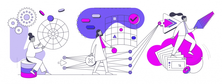
Jedoch ganz unabhängig von den Tools, gibt es eine ganz generelle Vorgehensweise in dieser datengetriebenen Prozessanalyse, die wir mit der folgenden Infografik beschreiben möchten.

DATANOMIQ Process Mining - 6 Steps of Doing Process Mining Analysis

6 Steps of Process Mining – Infographic PDF Download.

DATANOMIQ ist der herstellerunabhängige Beratungs- und Service-Partner für Business Intelligence, Process Mining und Data Science. Wir erschließen die vielfältigen Möglichkeiten durch Big Data und künstliche Intelligenz erstmalig in allen Bereichen der Wertschöpfungskette. Dabei setzen wir auf die besten Köpfe und das umfassendste Methoden- und Technologieportfolio für die Nutzung von Daten zur Geschäftsoptimierung.

Data Science & Big Data

Buzzword Bingo: Data Science – Teil II

Im ersten Teil unserer Serie „Buzzword Bingo: Data Science“ widmeten wir uns den Begriffen Künstliche Intelligenz, Algorithmen und Maschinelles Lernen. Nun geht es hier im zweiten Teil weiter mit der Begriffsklärung dreier weiterer Begriffe aus dem Data Science-Umfeld.

Buzzword Bingo: Data Science – Teil II: Big Data, Predictive Analytics & Internet of Things

Im zweiten Teil unserer dreiteiligen Reihe „Buzzword Bingo Data Science“ beschäftigen wir uns mit den Begriffen „Big Data“, „Predictive Analytics“ und „Internet of Things“.

Big Data

Interaktionen auf Internetseiten und in Webshops, Likes, Shares und Kommentare in Social Media, Nutzungsdaten aus Streamingdiensten wie Netflix und Spotify, von mobilen Endgeräten wie Smartphones oder Fitnesstrackern aufgezeichnete Bewegungsdate oder Zahlungsaktivitäten mit der Kreditkarte: Wir alle produzieren in unserem Leben alltäglich immense Datenmengen.

Im Zusammenhang mit künstlicher Intelligenz wird dabei häufig von „Big Data“ gesprochen. Und weil es in der öffentlichen Diskussion um Daten häufig um personenbezogene Daten geht, ist der Begriff Big Data oft eher negativ konnotiert. Dabei ist Big Data eigentlich ein völlig wertfreier Begriff. Im Wesentlichen müssen drei Faktoren erfüllt werden, damit Daten als „big“ gelten. Da die drei Fachbegriffe im Englischen alle mit einem „V“ beginnen, wird häufig auch von den drei V der Big Data gesprochen.

Doch welche Eigenschaften sind dies?

  • Volume (Datenmenge): Unter Big Data werden Daten(-mengen) verstanden, die zu groß sind, um sie mit klassischen Methoden zu bearbeiten, weil beispielsweise ein einzelner Computer nicht in der Läge wäre, diese Datenmenge zu verarbeiten.
  • Velocity (Geschwindigkeit der Datenerfassung und -verarbeitung): Unter Big Data werden Daten(-mengen) verstanden, die in einer sehr hohen Geschwindigkeit generiert werden und dementsprechend auch in einer hohen Geschwindigkeit ausgewertet und weiterverarbeitet werden müssen, um Aktualität zu gewährleisten.
  • Variety (Datenkomplexität oder Datenvielfalt): Unter Big Data werden Daten(-mengen) verstanden, die so komplex sind, dass auf den ersten Blick keine Zusammenhänge erkennbar sind. Diese Zusammenhänge können erst mit speziellen maschinellen Lernverfahren aufgedeckt werden. Dazu gehört auch, dass ein Großteil aller Daten in unstrukturierten Formaten wie Texten, Bildern oder Videos abgespeichert ist.

Häufig werden neben diesen drei V auch weitere Faktoren aufgezählt, welche Big Data definieren. Dazu gehören Variability (Schwankungen, d.h. die Bedeutung von Daten kann sich verändern), Veracity (Wahrhaftigkeit, d.h. Big Data muss gründlich auf die Korrektheit der Daten geprüft werden), Visualization (Visualisierungen helfen, um komplexe Zusammenhänge in großen Datensets aufzudecken) und Value (Wert, d.h. die Auswertung von Big Data sollte immer mit einem unternehmerischen Vorteil einhergehen).

Predictive Analytics

  • Heute schon die Verkaufszahlen von morgen kennen, sodass eine rechtzeitige Nachbestellung knapper Produkte möglich ist?
  • Bereits am Donnerstagabend die Regenwahrscheinlichkeit für das kommende Wochenende kennen, sodass passende Kleidung für den Kurztrip gepackt werden kann?
  • Frühzeitig vor bevorstehenden Maschinenausfällen gewarnt werden, sodass die passenden Ersatzteile bestellt und das benötigte technische Personal angefragt werden kann?

Als Königsdisziplin der Data Science gilt für viele die genaue Vorhersage zukünftiger Zustände oder Ereignisse. Im Englischen wird dann von „Predictive Analytics“ gesprochen. Diese Methoden werden in vielen verschiedenen Branchen und Anwendungsfeldern genutzt. Die Prognose von Absatzzahlen, die Wettervorhersage oder Predictive Maintenance (engl. für vorausschauende Wartung) von Maschinen und Anlagen sind nur drei mögliche Beispiele.

Zu beachten ist allerdings, dass Predictive-Analytics-Modelle keine Wahrsagerei sind. Die Vorhersage zukünftiger Ereignisse beruht immer auf historischen Daten. Das bedeutet, dass maschinelle Modelle mit Methoden des überwachten maschinellen Lernens darauf trainiert werden, Zusammenhänge zwischen vielen verschiedenen Eingangseigenschaften und einer vorherzusagenden Ausgangseigenschaft zu erkennen. Im Falle der Predicitve Maintenance könnten solche Eingangseigenschaften beispielsweise das Alter einer Produktionsmaschine, der Zeitraum seit der letzten Wartung, die Umgebungstemperatur, die Produktionsgeschwindigkeit und viele weitere sein. In den historischen Daten könnte ein Algorithmus nun untersuchen, ob diese Eingangseigenschaften einen Zusammenhang damit aufweisen, ob die Maschine innerhalb der kommenden 7 Tage ausfallen wird. Hierfür muss zunächst eine ausreichend große Menge an Daten zur Verfügung stehen. Wenn ein vorherzusagendes Ereignis in der Vergangenheit nur sehr selten aufgetreten ist, dann stehen auch nur wenige Daten zur Verfügung, um dasselbe Ereignis für die Zukunft vorherzusagen. Sobald der Algorithmus einen entsprechenden Zusammenhang identifiziert hat, kann dieses trainierte maschinelle Modell nun verwendet werden, um zukünftige Maschinenausfälle rechtzeitig vorherzusagen.

Natürlich müssen solche Modelle dauerhaft darauf geprüft werden, ob sie die Realität immer noch so gut abbilden, wie zu dem Zeitpunkt, zu dem sie trainiert worden sind. Wenn sich nämlich die Umweltparameter ändern, das heißt, wenn Faktoren auftreten, die zum Trainingszeitpunkt noch nicht bekannt waren, dann muss auch das maschinelle Modell neu trainiert werden. Für unser Beispiel könnte dies bedeuten, dass wenn die Maschine für die Produktion eines neuen Produktes eingesetzt wird, auch für dieses neue Produkt zunächst geprüft werden müsste, ob die in der Vergangenheit gefundenen Zusammenhänge immer noch Bestand haben.

Internet of Things

Selbstfahrende Autos, smarte Kühlschränke, Heizungssysteme und Glühbirnen, Fitnesstracker und vieles mehr: das Buzzword „Internet of Things“ (häufig als IoT abgekürzt) beschreibt den Trend, nicht nur Computer über Netzwerke miteinander zu verbinden, sondern auch verschiedene alltägliche Objekte mit in diese Netzwerke aufzunehmen. Seinen Anfang genommen hat dieser Trend in erster Linie im Bereich der Unterhaltungselektronik. In vielen Haushalten sind schon seit Jahren Fernseher, Computer, Spielekonsole und Drucker über das Heimnetzwerk miteinander verbunden und lassen sich per Smartphone bedienen.

Damit ist das IoT natürlich eng verbunden mit Big Data, denn all diese Geräte produzieren nicht nur ständig Daten, sondern sie sind auch auf Informationen sowie auf Daten von anderen Geräten angewiesen, um zu funktionieren.

Stop saying “trial and errors” for now: seeing reinforcement learning through some spectrums

*This is the fourth article of the series My elaborate study notes on reinforcement learning.

*In this article series “the book by Barto and Sutton” means “Reinforcement Learning: An Introduction second edition.” This book is said to be almost mandatory for those who seriously learn Reinforcement Learning (RL). And “the whale book” means a Japanese textbook named 「強化学習 (機械学習プロフェッショナルシリーズ)」(“Reinforcement Learning (Machine Learning Processional Series)”), by Morimura Tetsuro. I would say the former is for those who want to mainly learn how to use RL, and the latter is for more theoretical understanding. I am trying to make something between them in my series.

1, Finally to reinforcement learning

Some of you might have got away with explaining reinforcement learning (RL) only by saying an obscure thing like “RL enables computers to learn through trial and errors.” But if you have patiently read my articles so far, you might have come to say “RL is a family of algorithms which simulate procedures similar to dynamic programming (DP).” Even though my article series has not covered anything concrete and unique to RL yet, I think my series has already laid a hopefully effective foundation of discussions on RL. And in the first article, I already explained that “trial and errors” are only agents’ actions for collecting data from the environment. Such “trial and errors” lead to “experiences” of computers. And in this article we can finally start discussing how computers “experience” things in more practical and theoretical ways.

*The expression “to learn” is also frequently used in contexts of other machine learning algorithms. Thus in order to clearly separate the ideas, let me use the expression “to experience” when it comes to explaining RL. At any rate, what computers are doing is updating parameters, and in RL also updating values and policies. But some terms related to RL also use the word “experience,” for example experience replay, so “to experience” might be a preferred phrase in RL fields.

I think changing discussions on DP into those on RL is like making graphs more “open” rather than “closed.” In the second article, I explained DP problems, where the models of environments are completely known, as repeatedly updating graphs like neural networks. As I have been repeatedly saying RL, or at least model-free RL, is an approximated application of DP in the environments without a complete model. That means, connections of nodes of the graph, that is relations of actions and states, are something agents have to estimate directly or indirectly. I think that can be seen as untying connections of the graphs which I displayed when I explained DP. By doing so, I propose to see RL or more exactly model-free RL like the graph of the right side of the figure below.
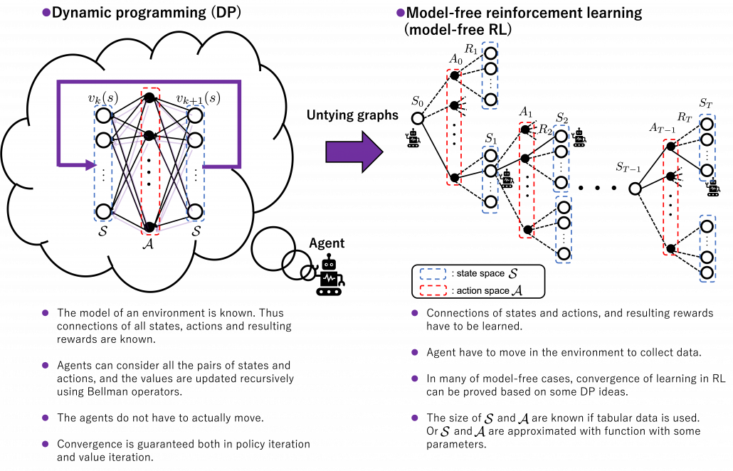
*For the time being, I would prefer to use the term model-free RL rather than just RL. That is not only because this article is about model-free RL but also because I want to avoid saying inaccurate things about wider range of RL algorithms I would have to study more precisely and explain.

Some people might say these are tree structures, and that might be technically correct. But in my sense, this is more of “willows.” The cover of the second edition of the books by Barto and Sutton also looks like willows. The cover design comes from a paper on RL named “Learning to Drive a Bicycle using Reinforcement Learning and Shaping.” The paper is about learning to ride a bike in a simulator with RL. The geometric patterns are not models of human brain nerves, but trajectories of an agent learning to balance a bike. However interestingly, the trajectories of the bike, which are inscribed on a road, partly diverge but converge in a certain way as a whole, like the RL graph I propose. That is why I chose some pictures of 「花札 (hanafuda)」as the main picture of this series. Hanafuda is a Japanese gamble card game with monthly seasonal flower pictures. And the cards of June have pictures of willows.

Source: Learning to Drive a Bicycle using Reinforcement Learning and Shaping, Randløv, (1998)    Richard S. Sutton, Andrew G. Barto, “Reinforcement Learning: An Introduction,” MIT Press, (2018)

2, Untying DP graphs: planning or learning

Even though I have just loudly declared that my RL graphs are more of “willow” structures in my aesthetic sense, I must admit they should basically be discussed as popular tree structures. That is because, when you start discussing practical RL algorithms you need to see relations of states and actions as tree structures extending. If you already more or less familiar with tree structures or searching algorithms on tree graphs, learning RL with tree structures should be more or less straightforward to you. Another reason for using tree structures with nodes of states and actions is that the book by Barto and Sutton use buck up diagrams of Bellman equations which are tree graphs. But I personally think the graphs should be used more effectively, so I am trying to expand its uses to DP and RL algorithms in general. In order to avoid confusions about current discussions on RL in my article series, I would like to give an overall review on how to look at my graphs.

The graphs in the figure below are going to be used in my articles, at least when I talk about model-free RL. I made them based on the backup diagram of Bellman equation introduced in the book by Barto and Sutton. I would like you to first remember that in RL we are basically discussing Markov decision process (MDP) environment, where the next action and the resulting next states depends only on the current state. Such models are composed of white nodes representing each state s in an state space \mathcal{S}, and black nodes representing each action a, which is a member of an action space \mathcal{A}. Any behaviors of agents are represented as going back and forth between black and white nodes of the model, and that is why connections in the MDP model are bidirectional.  In my articles let me call such model of environments “a closed model.” RL or general planning problems are matters of optimizing policies in such models of environments. Optimizing the policies are roughly classified into two types, planning/searching or RL, and the main difference between them is whether connections of graphs of models are known or not. Planning or searching is conducted without actually moving in the environment. DP are family of planning algorithms which are known to converge, and so far in my articles we have seen that DP are enabled by repeatedly applying Bellman operators. But instead of considering and updating all the possible transitions in the model like DP, planning can be conducted more sparsely. Such sparse planning are often called searching, and many of them use tree structures. If you have learned any general decision making problems with tree graphs, you might be already familiar with some searching techniques like alpha-beta pruning.
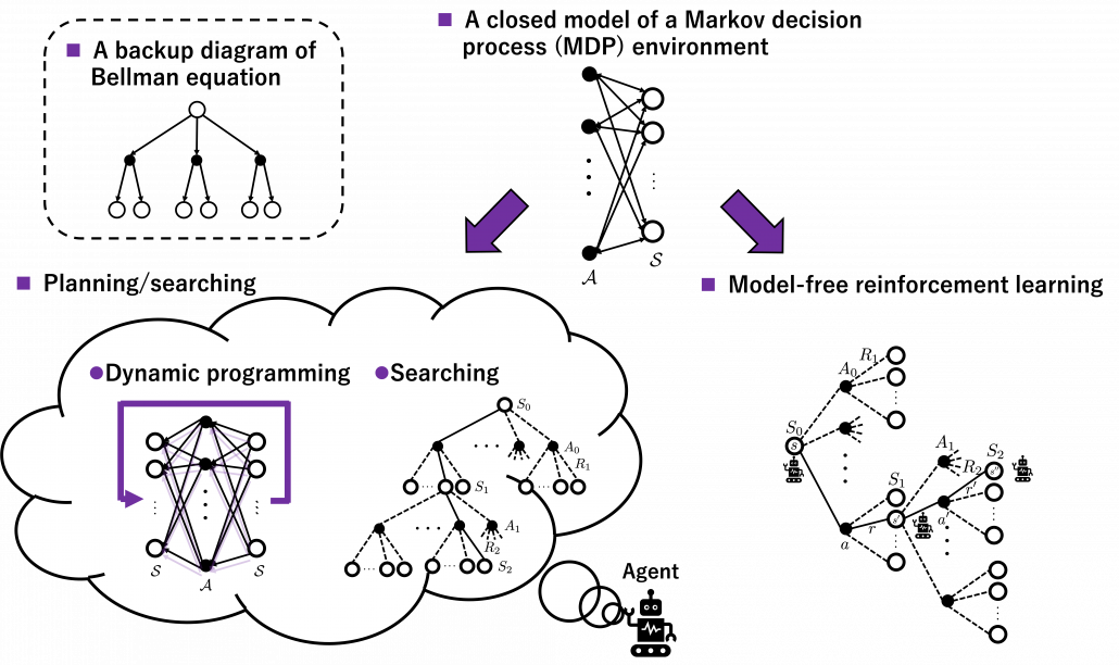
*In explanations on DP in my articles, directions of connections of model graphs are confusing, so I precisely explained how to look at them in the second section in the last article.

On the other hand, RL algorithms are matters of learning the linkages of models of environments by actually moving in them. For example, when the agent in the figure below move on a grid map like the purple arrows, the movement is represented like in the closed model in the middle. However as the agent does not have the complete closed model, the agent has to move around in the environment like the tree structure at the right side to learn values of each node.
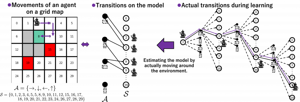
The point is, whether models of environments are known or unknown, or whether agents actually move in the environment or not, movements of agents are basically represented as going back and forth between white nodes and black nodes in closed models. And such closed models are entangled in searching or RL. They are similar operations, but they are essentially different in that searching agents do not actually move in searching but in RL they actually move.  In order to distinguish searching and learning, in my articles, trees for searching are extended vertically, trees for learning horizontally.

*DP and searching are both planning, but DP consider all the connections of actions and states by repeatedly applying Bellman operators. Thus I would not count DP as “untying” of closed models.

3, Some spectrums in RL algorithms

Starting studying actual RL algorithms also means encountering various algorithms one after another. Some of you might have already been overwhelmed by new terms coming up one after another in study materials on RL. That is because, as I explained in the first article, RL is more about how to train models of values or policies. Thus it is natural that compared to general machine learning, which more or less share the same training frameworks, RL has a variety of training procedures. Rather than independently studying each RL algorithm, I think it is more effective to see connections of each algorithm, which is linked by adjusting degrees of some important elements in RL. In fact I have already introduced those elements as some pairs of key words of RL in the first article. But it would be all the more effective to review them, especially after learning DP algorithms as representative planning methods. If you study RL that way, you would come to see trial and errors or RL as a crucial but just one aspect of RL.
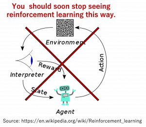
I think if you care less about the trial-and-error aspect of RL that allows you to study RL more effectively in the beginning. And for the time being, you should stop viewing RL in the popular way as presented above. Not that I am encouraging you to ignore the trial and error part, namely relations of actions, rewards, and states. My point is that it is more of inside the agent that should be emphasized. Planning, including DP is conducted inside the agent, and trial and errors are collection of data from the environment for the sake of the planning. That is why in many study materials on RL, DP is first introduced. And if you see differences of RL algorithms as adjusting of some pairs of elements of planning problems, it would be less likely that you would get lost in curriculums on RL. The pairs are like some spectrums. Not that you always have to choose either of each pair, but rather ideal solutions are often in the middle of the two ends of the spectrums depending on tasks. Let’s take a look at the types of those spectrums one by one.

(1) Value-policy or actor-critic spectrum

The crucial type of spectrum you should be already familiar with is the value-policy one. I think this spectrum can be adjusted in various ways. For example, over the last two articles we have seen how values and policies reach the optimal functions in DP using policy iteration or value iteration. Policy iteration alternates between updating values and policies until convergence to the optimal policy, whereas value iteration keeps updating only values until reaching the optimal value, to get the optimal policy at the end. And similar discussions can be seen also in the upcoming RL algorithms. The book by Barto and Sutton sees such operations in general as generalized policy iteration (GPI).
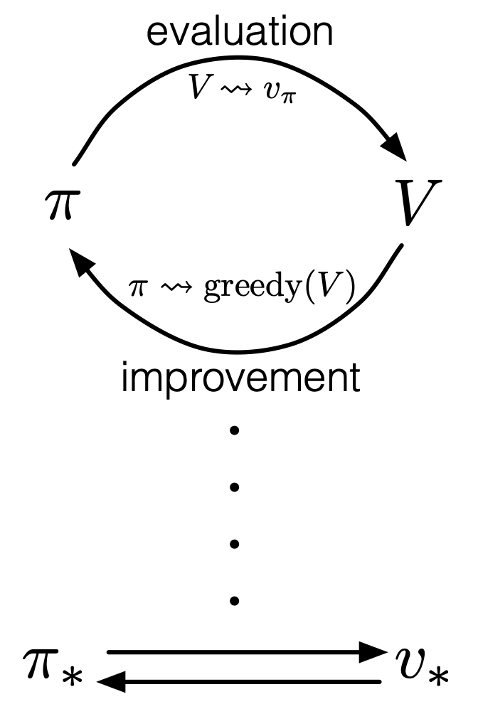
Source: Richard S. Sutton, Andrew G. Barto, “Reinforcement Learning: An Introduction,” MIT Press, (2018)

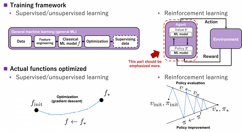
You should pay attention to the idea of GPI because this is what makes RL different form other general machine learning. In many cases RL is explained as a field of machine learning which is like trial and errors, but I personally think that GPI, interactive optimization between values and policies, should be more emphasized. As I said in the first article, RL optimizes decision making rules, that is policies \pi(a|s), in MDPs. Other general machine learning algorithms have more direct supervision by loss functions and models are optimized so that loss functions are minimized. In the case of the figure below, an ML model f is optimized to f_{\ast} by optimization such as gradient descent. But on the other hand in RL policies \pi do not have direct loss functions. Then RL uses values v(s), which are functions of how good it is to be in states s. As one part of GPI, the value function v_{\pi} for the current policy \pi is calculated, and this is called estimation in the book by Barto and Sutton.  And based on the estimated value function, the policy is improved as \pi ', which is called policy improvement, and overall processes of estimation and policy improvement are called control in the book. And v_{\pi} and \pi are updated alternately this way until converging to the optimal values v_{\ast} or policies \pi_{\ast}. This interactive updates of values and policies are done inside the agent, in the dotted frame in red below. I personally think this part should be more emphasized than trial-and-error-like behaviors of agents. Once you see trial and errors of RL as crucial but just one aspect of GPI and focus more inside agents, you would see why so many study materials start explaining RL with DP.
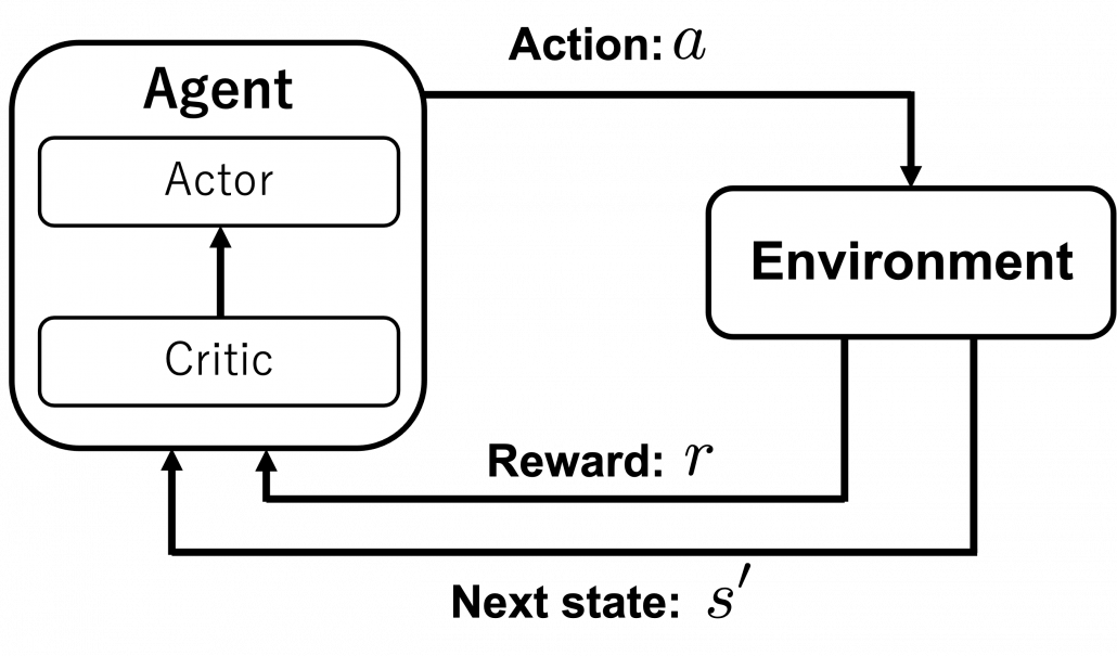
You can explicitly model such interactions of values and policies by modeling each of them with different functions, and in this case such frameworks of RL in general are called actor-critic methods. I am gong to explain actor-critic methods in an upcoming article. Thus the value-policy spectrum also can be seen as a actor-critic spectrum. Differences between the pairs of value-policy or actor-critic spectrums are something you would little by little understand. For now I would say GPI is the most general and important idea behind RL. But practical RL algorithms are implemented as actor-critic methods. Critic parts gives some signals to actor parts, and critic parts get its consequence by actor parts taking actions in environments. Not that actors directly give feedback to critics.
*I think one of confusions in studying RL come from introducing Q-learning or SARSA at the first algorithms or a control in RL. As I have said earlier, interactive relations between values and policies or actors and critics, that is GPI, should be emphasized. And I think that is why DP is first introduced in many books. But in Q-learning or SARSA, an actor and a critic parts are combined as one module. But explicitly separating the actor and critic parts would be just too difficult at the beginning. And modeling an actor and a critic with separate modules would lead to difficulties in optimizing them together.

(2) Exploration-exploitation or on-off policy spectrum

I think the most straightforward spectrum is the exploitation-exploration spectrum. You can adjust how likely agents take random actions to collect data. Occasionally it is ideal for agents to have some degree of randomness in taking actions to explore unknown states of environments. One of the simplest algorithms to formulate randomness of actions is ε-greedy method, which I explained in the first article. In this method in short agents take a random action with a probability of ε. Instead of arbitrarily setting a hyperparameter \epsilon, randomness of actions can be also learned by modeling policies with certain functions. This randomness of functions can be also modeled in actor-critic frameworks. That means, depending on a choice of an actor, such actor can learn randomness of actions, that is explorations.

The two types of spectrums I have introduced so far lead to another type of spectrum. It is an on-off policy spectrum. Even though I explained types of policies in the last article using examples of home-lab-Starbucks diagrams, there is another way to classify policies: there are target policies and behavior policies. The former are the very policies whose optimization we have been discussing. The latter are policies for taking actions and collecting data. When agents use target policies also as behavior policies, they are on-policy algorithms. If agents use different policies for taking actions during optimization of target policies, they are off-policy methods.
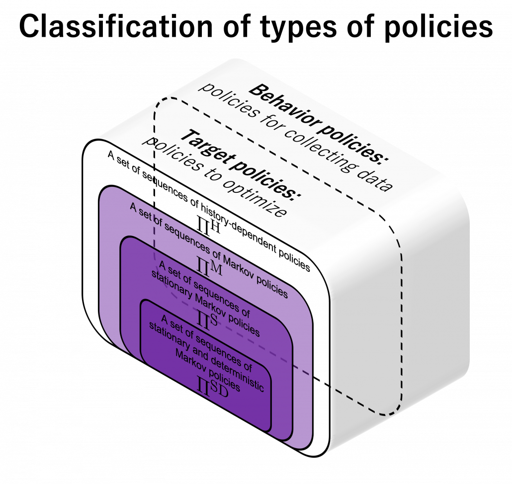
Policy iteration and value iteration of DP can be also classified into on-policy or off-policy in a sense. In policy iteration values are updated using an up-to-date estimated policy, and the policy becomes optimal when it converges. Thus behavior and target policies are the same in this case. On the other hand in value iteration, values are updated with Bellman optimality operator, which updates values in a greedy way. Using greedy method means the policy \pi is not used for considering which action to take. Thus target and behavior policies are different. As you will see soon, concrete model-free RL algorithms like SARSA or Q-learning also have the same structure: the former is on-policy and the latter is off-policy. The difference of on-policy or off-policy would be more straightforward if we model behavior policies and target policies with different functions. An advantage of off-policy RL is you can model randomness of exploration of agents with extra functions. On the other hand, a disadvantage is that it would be harder to train different models at the same time. That might be a kind of tradeoff similar to an actor-critic method.

Even though this exploration-exploitation aspect of RL is relatively easy to understand, at the same time that can lead to much more complicated discussions on RL, which I would not be able to cover in this article series. I recommended you to stop seeing RL as trial and errors for the time being, but in the end trial and errors would prove to be crucial because data needed for GPI are collected mainly via trial and errors. Even if you implement some simple RL algorithms, you would soon realize it is hard to deal with unvisited states. Enough explorations need to be modeled by a behavior policy or some sophisticated heuristic techniques. I am planning to explain convergence of several RL algorithms, and they are guaranteed by sufficiently exploring all the states. However, thorough explorations of all the states lead to massive computational costs. But lack of exploration would let RL agents myopically overestimate current policies, never finding policies which pay off in the long run. That might be close to discussions on how to efficiently find a global minimum of a loss function, avoiding local minimums.

(3) TD-MonteCarlo spectrum

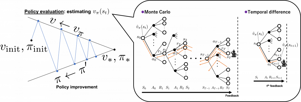
A variety of spectrums so far are enabled by modeling proper functions on demand. But in AI problems such functions are something which have to be automatically trained with some supervision. Instead of giving supervision explicitly with annotated data like in supervised learning of general machine learning, RL agents train models with “experiences.” As I am going to explain in the next part of this article, “experiences” in RL contexts mean making some estimations of values and adjusting such estimations based on actual rewards they get. And the timings of such feedback lead to another spectrum, which I call a TD-MonteCarlo spectrum. When the feedback happens every time an agent takes an action, it is TD method, on the other hand when that happens only at the end of an episode, that is Monte Carlo method. But it is easy to imagine that ideal solutions are usually at the middle of them. I am going to dig this topic soon in the next article. And n-step methods or TD(λ), which bridge the TD and Monte Carlo, are going to be covered in one of upcoming articles.
(4) Model free-based spectrum

The next spectrum might be relatively hard to understand, and to be honest I am still not completely sure about this topic. Please bear that in your mind. In the last section, I said RL is a kind of untying DP graphs and make them open because in RL, models of environments are unknown. However to be exact, that was mainly about model-free RL, which this article is going to cover for the time being. And I would say the graphs I showed in the last section were just two extremes of this model based-free spectrum. Some model-based RL methods exist in the middle of those two ends. In short RL agents can retain models of environments and do some plannings even when they do trial and errors. The figure below briefly compares planning, model-based RL, and model-free RL in the spectrum.
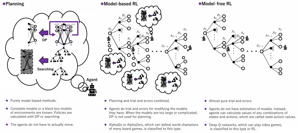
Let’s take a rough example of humans solving a huge maze. DP, which I have covered is like having a perfect map of the maze and making plans of how to move inside in advance. On the other hand, model-free reinforcement learning is like soon actually entering the maze without any plans. In model-free reinforcement learning, you only know how big the maze is, and you have a great memory for remembering in which directions to move, in all the places. However, as the model of how paths are connected is unknown, and you naively try to remember all the actions in all the places, it generally takes a longer time to solve the maze. As you could easily imagine, having some heuristic ideas about the model of the maze and taking some notes and making plans about courses would be the most efficient and the most peaceful. And such models in your head can be updated by actually moving in the maze.

*I believe that you would not say the pictures above are spoilers.

I need to more clearly talk about what a model is in RL or general planning problems. The book by Barto and Sutton simply defines a model this way: “By a model of the environment we mean anything that an agent can use to predict how the environment will respond to its actions. ” The book also says such models can be also classified to distribution models and sample models. The difference between them is the former describes an environment as combinations of known models, but the latter is like a black box model of an environment. An intuitive example is, as introduced in the book by Barto and Sutton, throwing dozens of dices can be seen in the both types. If you just throw the dices, sometimes chancing numbers of dices, and record the sum of the numbers on the dices s every time, that is equal to getting the sum from a black box. But a probabilistic distribution of such sums can be actually calculated as a multinomial distribution. Just as well, you can see a probability of transitions in an RL environment as a black box, but the probability can be also modeled. Some readers might have realized that distribution or sample models can be almost the same in the end, with sufficient data. In many cases of machine learning or statistics algorithms, complicated distributions have to be approximated with samples. Or rather how to approximate them is more of interest. In the case of dozens of dices, you can analytically calculate its distribution model as a multinomial distribution. But if you throw the dices numerous times, you would get precise approximated distributions.

When we discuss model-based RL, we need to consider not only DP but also other planning algorithms. DP is a family of planning algorithms which are known to converge, and many of RL algorithms share a lot with DP at theoretical levels. But in fact DP has one shortcoming even if the MDP model of an environment is known: DP needs to consider and update all the states. When models of environments are too complicated and large, applying DP is not a good idea. Also in many of such cases, you could not even get such a huge model of the environment. You would rather get only a black box model of the environment. Such a black box model only gets a pair of current state and action (s, a), and gives out the next state s' and corresponding reward r, that is the black box is a sample model. In this case other planning methods with some searching algorithms are used, for example Monte Carlo tree search. Such search algorithms are designed to more efficiently and sparsely search states and actions of interest. Many of searching algorithms used in RL make uses of tree structures. Model-based approaches can be roughly classified into three types below based on size or complication of models.
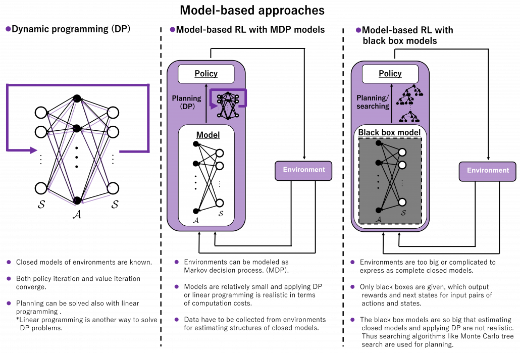
*As you could see, differences between sample models and distribution models can be very ambiguous. So are differences between model-free and model-based RL, I guess. As a matter of fact the whale book says the distributions of models approximated in model-free RL are the same as those in model-based ones. I cannot say anything exactly anymore, but I guess model-free RL is more of “memorizing” an environment, or combinations of states and actions in the environments. But memorizing environments can be computationally problematic in many cases, so assuming some distributions of models can help. That is my impression for now.

*Tree search algorithms alone shows very impressive performances, as long as you have massive computation resources. A heuristic tree search without reinforcement learning could defeat Garri Kasparow, a former chess champion, as long as enough computation resource is available. Searching algorithms were enough for “simplicity” of chess.

*I am not sure whether model-free RL algorithms are always simpler than model-based ones. For example Deep Q-Learning, a model-free method with some neural networks can learn to play Atari or Nintendo Entertainment System. Model-based deep RL is used in more complex task like AlphaGo or AlphaZero, which can defeat world champions of various board games. AlphaGo or AlphaZero models intuitions in phases of board games with convolutional neural networks (CNN), prediction of some phases ahead with search algorithms, and learning from past experiences with RL. I am not going to cover model-based RL in general in this series, but instead I would like to explain how RL enables computers to play video games after introducing some searching algorithms.

(5) Model expressivity spectrum

No matter how impressive or dreamy RL algorithms sound, their competence largely depend on model expressivity. In the first article, I emphasized “simplicity” of RL. DP or RL algorithms so far or in upcoming several articles consider incredibly simple cases like kids playbooks. And that beginning parts of most RL study materials cover only the left side of the figure below. In order to enable RL agents with more impressive tasks such as balancing cart-pole or playing video games, we need to raise the bar of expressivity spectrum, from the left to the right side of the figure below. You need to wait until a chapter or a section on “function approximation” in order to actually feel that your computer is doing trial and errors. And such chapters finally appear after reading half of both the book by Barto and Sutton and the whale book.
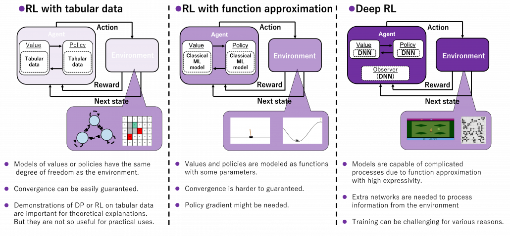
*And this spectrum is also a spectrum of computation costs or convergence. The left type could be easily implemented like programming assignments of schools since it in short needs only Excel sheets, and you would soon get results. The middle type would be more challenging, but that would not b computationally too expensive. But when it comes to the type at the right side, that is not something which should be done on your local computer. At least you need a GPU. You should expect some hours or days even for training RL agents to play 8 bit video games. That is of course due to cost of training deep neural networks (DNN), especially CNN. But another factors is potential inefficiency of RL. I hope I could explain those weak points of RL and remedies for them.

We need to model values and policies with certain functions. For the time being, in my articles values and policies are just modeled as tabular data, that is some NumPy arrays or Excel sheets. These are types of cases where environments and actions are relatively simple and discrete. Thus they can be modeled with some tabular data with the same degree of freedom. Assume a case where there are only 30 grids in an environment and only 4 types of actions in every grid. In such case, values are stored as arrays with 30 elements, and so are policies. But when environments are more complex or require continuous values of some parameters, values and policies have to be approximated with some models. When only relatively few parameters need to be estimated, simple machine learning models such as softmax functions can be used as such models. But compared to the cases with tabular data, convergence of training has to be discussed more carefully. And when you need to estimate continuous values, techniques like policy gradients have to be introduced. And we can dramatically enhance expressivity of models with deep neural netowrks (DNN), and such RL is called deep RL. Deep RL has showed great progress these days, and it is capable of impressive performances. Deep RL often needs observers to process inputs like video frames, and for example convolutional neural networks (CNN) can be used to make such observers. At any rate, no matter how much expressivity RL models have, they need to be supervised with some signals just as general machine learning often need labeled data. And “experiences” give such supervisions to RL agents.

(6) Adjusting sliders of spectrum

As you might have already noticed, these spectrums are not something you can adjust independently like faders on mixing board. They are more like some sliders for adjusting colors, brightness, or chroma on painting software. If you adjust one element, other parts are more or less influenced. And even though there are a variety of colors in the world, they continuously change by adjusting those elements of colors. Just as well, even if each RL algorithms look independent, many of them share more or less the same ideas, and only some parts are different in terms of their degrees. When you get lost in the course of studying RL, I would like you to decompose the current topic into these spectrums of RL elements I have explained.
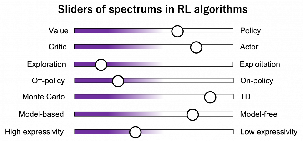
I hope my explanations so far changed how you see RL. In the first article I already said RL is approximation of DP-like procedures with data collected by trial and errors, but from now on I would explain it also this way: RL is a family of algorithms which enable GPI by adjusting some spectrums.

In the next some articles, I am going to mainly cover RL algorithms named SARSA and Q-learning. Both of them use tabular data, and they are model-free. And in values and policies, or actors and critics are together modeled as action-value functions, which I am going to explain later in this article. The only difference is SARSA is on-policy, and Q-learning is off-policy, just as I have already mentioned. And when it comes to how to train them, they both use Temporal Difference (TD), and this gives signals of “experience” to RL agents. Altering DP in to model-free RL is, in the figure above, adjusting the model-based-free and MonteCarlo-TD spectrums to the right end. And you also adjust the low-high-expressivity and value-policy spectrums to the left end. In terms of actor-critic spectrum, the actor and the critic parts are modeled as the same module. Seeing those algorithms this way would be much more effective than looking at their pseudocode independently.

* I make study materials on machine learning, sponsored by DATANOMIQ. I do my best to make my content as straightforward but as precise as possible. I include all of my reference sources. If you notice any mistakes in my materials, including grammatical errors, please let me know (email: yasuto.tamura@datanomiq.de). And if you have any advice for making my materials more understandable to learners, I would appreciate hearing it.

Training of Deep Learning AI models

It’s All About Data: The Training of AI Models

In deep learning, there are different training methods. Which one we use in an AI project depends on the data provided by our customer: how much data is there, is it labeled or unlabeled? Or is there both labeled and unlabeled data?

Let’s say our customer needs structured, labeled images for an online tourism portal. The task for our AI model is therefore to recognize whether a picture is a bedroom, bathroom, spa area, restaurant, etc. Let’s take a look at the possible training methods.

1. Supervised Learning

If our customer has a lot of images and they are all labeled, this is a rare stroke of luck. We can then apply supervised learning. The AI model learns the different image categories based on the labeled images. For this purpose, it receives the training data with the desired results from us.

During training, the model searches for patterns in the images that match the desired results, learning the characteristics of the categories. The model can then apply what it has learned to new, unseen data and in this way provide a prediction for unlabeled images, i.e., something like “bathroom 98%.”

2. Unsupervised Learning

If our customer can provide many images as training data, but all of them are not labeled, we have to resort to unsupervised learning. This means that we cannot tell the model what it should learn (the assignment to categories), but it must find regularities in the data itself.

Contrastive learning is currently a common method of unsupervised learning. Here, we generate several sections from one image at a time. The model should learn that the sections of the same image are more similar to each other than to those of other images. Or in short, the model learns to distinguish between similar and dissimilar images.

Although we can use this method to make predictions, they can never achieve the quality of results of supervised learning.

3. Semi-supervised Learning

If our customer can provide us with few labeled data and a large amount of unlabeled data, we apply semi-supervised learning. In practice, we actually encounter this data situation most often.

With semi-supervised learning, we can use both data sets for training, the labeled and the unlabeled data. This is possible by combining contrastive learning and supervised learning, for example: we train an AI model with the labeled data to obtain predictions for room categories. At the same time, we let the model learn similarities and dissimilarities in the unlabeled data and then optimize itself. In this way, we can ultimately achieve good label predictions for new, unseen images.

Supervised vs. Unsupervised vs. Semi-supervised

Everyone who is entrusted with an AI project wants to apply supervised learning. In practice, however, this is rarely the case, as rarely all training data is well structured and labeled.

If only unstructured and unlabeled data is available, we can at least extract information from the data with unsupervised learning. These can already provide added value for our customer. However, compared to supervised learning, the quality of the results is significantly worse.

With semi-supervised learning, we try to resolve the data dilemma of small part labeled data, large part unlabeled data. We use both datasets and can obtain good prediction results whose quality is often on par with those of supervised learning. This article is written in cooperation between DATANOMIQ and pixolution, a company for computer vision and AI-bases visual search.

Buzzword Bingo: Data Science – Teil I

Rund um das Thema Data Science gibt es unglaublich viele verschiedene Buzzwords, die Ihnen sicherlich auch schon vielfach begegnet sind. Sei es der Begriff Künstliche Intelligenz, Big Data oder auch Deep Learning. Die Bedeutung dieser Begriffe ist jedoch nicht immer ganz klar und häufig werden Begriffe auch vertauscht oder in missverständlichen Zusammenhängen benutzt. Höchste Zeit also, sich einmal mit den genauen Definitionen dieser Begriffe zu beschäftigen!

Buzzword Bingo: Data Science – Teil 1: Künstliche Intelligenz, Algorithmen & Maschinelles Lernen

Im ersten Teil unserer dreiteiligen Reihe „Buzzword Bingo Data Science“ beschäftigen wir uns zunächst mit den drei Begriffen „Künstliche Intelligenz“, „Algorithmus“ und „Maschinelles Lernen“.

Künstliche Intelligenz

Der im Bereich der Data Science u. a. am häufigsten genutzte Begriff ist derjenige der „Künstlichen Intelligenz“. Viele Menschen denken bei dem Begriff sofort an hochspezialisierte Maschinen à la „The Matrix“ oder „I, Robot“. Dabei ist der Begriff deutlich älter als viele denken. Bereits 1956 wurde der englische Begriff “artificial intelligence” zum ersten Mal in einem Workshop-Titel am US-amerikanischen Dartmouth College genutzt.

Heutzutage besitzt der Begriff der künstlichen Intelligenz keine allgemeingültige Definition. Es handelt sich bei künstlicher Intelligenz grundsätzlich um ein Teilgebiet der Informatik, das sich mit der Automatisierung von intelligentem Verhalten befasst. Es geht also darum, dass ein Computerprogramm auf eine Eingabe eine intelligente Reaktion zeigt. Zu beachten ist hierbei, dass eine künstliche Intelligenz nur ein scheinbar intelligentes Verhalten zeigen kann. Künstliche Intelligenz wird heutzutage sehr weit gefasst und kann vieles umfassen: von klassischen, regelbasierten Algorithmen bis hin zu selbstlernenden künstlichen neuronalen Netzen.

Das zentrale Forschungsziel ist die Entwicklung einer sogenannten Allgemeinen Künstlichen Intelligenz, also einer Maschine, die in der Lage sein wird, autonom beliebige Probleme zu lösen. Es gibt eine fortlaufende Debatte darüber, ob dieses Ziel jemals erreicht werden kann bzw. ob es erreicht werden sollte.

In den vergangenen Jahren ist auch die sogenannte xAI (engl. Explainable AI; erklärbare künstliche Intelligenz) in den Mittelpunkt der Forschungsinteressen gerückt. Dabei geht es um die Problematik, dass künstliche Intelligenzen sogenannte Black Boxen sind. Das bedeutet, dass ein menschlicher User die Entscheidung einer künstlichen Intelligenz üblicherweise nicht nachvollziehen kann. Eine xAI wäre im Vergleich jedoch eine Glass Box, die Entscheidungen einer solchen künstlichen Intelligenz wären für Menschen also nachvollziehbar.

Algorithmen

Algorithmen sind klar definierte, vorgegebene Prozeduren, mit denen klar definierte Aufgaben gelöst werden können. Dabei kann der Lösungsweg des Algorithmus entweder durch Menschen vorgegeben, also programmiert werden oder Algorithmen lernen durch Methoden des maschinellen Lernens selbstständig den Lösungsweg für eine Prozedur.

Im Bereich der Data Science bezeichnen wir mit Algorithmen kleine Programme, die scheinbar intelligent handeln. Dementsprechend stecken auch hinter künstlichen Intelligenzen Algorithmen. Werden Algorithmen mit klar definierten Eingaben versorgt, führen sie somit zu einem eindeutigen, konstanten Ergebnis. Dabei gilt aber leider auch der Grundsatz der Informatik „Mist rein, Mist raus“. Ein Algorithmus kann immer nur auf sinnvolle Eingaben sinnvolle Ausgaben erzeugen. Die Komplexität von Algorithmen kann sehr vielfältig sein und je komplexer ein solcher Algorithmus ist, desto „intelligenter“ erscheint er oftmals.

Maschinelles Lernen

Maschinelles Lernen ist ein Überbegriff für eine Vielzahl von Verfahren, mit denen ein Computer oder eine künstliche Intelligenz automatisch Muster in Daten erkennt. Beim maschinellen Lernen wird grundsätzlich zwischen dem überwachten und unüberwachten Lernen unterschieden.

Beim überwachten Lernen lernt ein Algorithmus den Zusammenhang zwischen bekannten Eingabe- und Ausgabewerten. Nachdem dieser Zusammenhang vom Algorithmus erlernt wurde, kann dieses maschinelle Modell dann auf neue Eingabewerte angewandt und somit unbekannte Ausgabewerte vorhergesagt werden. Beispielsweise könnte mithilfe einer Regression zunächst der Zusammenhang zwischen Lufttemperatur und dem Wochentag (jeweils bekannte Eingabewerte) sowie der Anzahl der verkauften Eiskugeln (für die Vergangenheit bekannte Ausgabewerte) in einem Freibad untersucht werden. Sobald dieser Zusammenhang einmal ausreichend genau bestimmt worden ist, kann er auch für die Zukunft fortgeschrieben werden. Das bedeutet, es wäre dann möglich, anhand des nächsten Wochentages sowie der vorhergesagten Lufttemperatur (bekannte Eingabewerte für die Zukunft) die Anzahl der verkauften Eiskugeln (unbekannte Ausgabewerte für die Zukunft) zu prognostizieren und somit die Absatzmenge genauer planen zu können.

Beim unüberwachten Lernen auf der anderen Seite sind nur Eingabedaten vorhanden, es gibt keine den Eingabedaten zugehörigen Ausgabedaten. Hier wird dann mit Methoden wie beispielsweise dem Clustering versucht, verschiedene Datenpunkte anhand ihrer Eigenschaften in verschiedene Gruppen aufzuteilen. Beispielsweise könnte ein Clustering-Algorithmus verschiedene Besucher:innen eines Webshops in verschiedene Gruppen einteilen: Es könnte beispielsweise eine Gruppe von Besucher:innen geben, die sehr zielstrebig ein einzelnes Produkt in den Warenkorb legen und ihren Kauf direkt abschließen. Andere Besucher:innen könnten allerdings viele verschiedene Produkte ansehen, in den Warenkorb legen und am Ende nur wenige oder vielleicht sogar gar keine Käufe tätigen. Wieder andere Kund:innen könnten unter Umständen lediglich auf der Suche nach Artikeln im Sale sein und keine anderen Produkte ansehen.

Aufgrund ihres Nutzungsverhaltens auf der Website könnte ein Clustering-Algorithmus mit ausreichend aufbereiteten Daten nun all diese Kund:innen in verschiedene Gruppen oder Cluster einteilen. Was der Algorithmus jedoch nicht leisten kann ist zu erklären, was die erkannten Cluster genau bedeuten. Hierfür braucht es nach wie vor menschliche Intelligenz gepaart mit Fachwissen.

Automatic Financial Trading Agent for Low-risk Portfolio Management using Deep Reinforcement Learning

This article focuses on autonomous trading agent to solve the capital market portfolio management problem. Researchers aim to achieve higher portfolio return while preferring lower-risk actions. It uses deep reinforcement learning Deep Q-Network (DQN) to train the agent. The main contribution of their work is the proposed target policy.
Introduction

Author emphasizes the importance of low-risk actions for two reasons: 1) the weak positive correlation between risk and profit suggests high returns can be obtained with low-risk actions, and 2) customer satisfaction decreases with increases in investment risk, which is undesirable. Author challenges the limitation of Supervised Learning algorithm since it requires domain knowledge. Thus, they propose Reinforcement Learning to be more suitable, because it only requires state, action and reward specifications.

The study verifies the method through the back-test in the cryptocurrency market because it is extremely volatile and offers enormous and diverse data. Agents then learn with shorter periods and are tested for the same period to verify the robustness of the method. 

2 Proposed Method

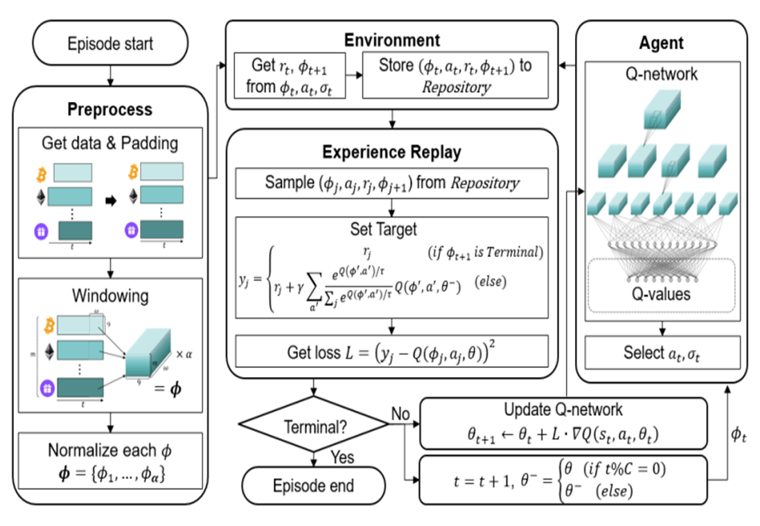
The overall structure of the proposed method is shown below.

The architecutre of the proposed trading agent system.
The architecutre of the proposed trading agent system.

2.1 Problem Definition

The portfolio consists of m assets and one base currency.

The price vector p stores the price p of all assets:

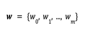
The portfolio vector w stores the amount of each asset:

At time 𝑡, the total value W_t of the portfolio is defined as the inner product of the price vector p_t and the portfolio vector w_t .

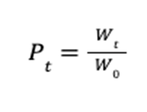
Finally, the goal is to maximize the profit P_t at the terminal time step 𝑇.

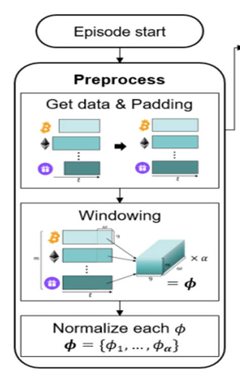
2.2 Asset Data Preprocessing

1) Asset Selection
Data is drawn from the Binance Exchange API, where top m traded coins are selected as assets.

2) Data Collection
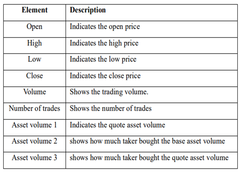
Each coin has 9 properties, shown in Table.1, so each trade history matrix has size (α * 9), where α is the size of the target period converted into minutes.

3) Zero-Padding
Pad all other coins to match the matrix size of the longest coin. (Coins have different listing days)

Comment: Author pointed out that zero-padding may be lacking, but empirical results still confirm their method covering the missing data well.

4) Stack Matrices
Stack m matrices of size (α * 9) to form a block of size (m* α * 9). Then, use sliding window method with widow size w to create (α – w + 1) number of sequential blocks with size (w *  m * 9).

5) Normalization
Normalize blocks with min-max normalization method. They are called history block 𝜙 and used as input (ie. state) for the agent.

3. Deep Q-Network

The proposed RL-based trading system follows the DQN structure.

Deep Q-Network has 2 networks, Q- and Target network, and a component called experience replay. The Q-network is the agent that is trained to produce the optimal state-action value (aka. q-value).

Comment: Q-value is calculated by the Bellman equation, which, in short, consists of the immediate reward from next action, and the discounted value of the next state by following the policy for all subsequent steps.


Here,
Agent: Portfolio manager
Action a: Trading strategy according to the current state
State 𝜙 : State of the capital market environment
Environment: Has all trade histories for assets, return reward r and provide next state 𝜙’ to agent again

DQN workflow:

DQN gets trained in multiple time steps of multiple episodes. Let’s look at the workflow of one episode.

Training of a Deep Q-Network

Training of a Deep Q-Network

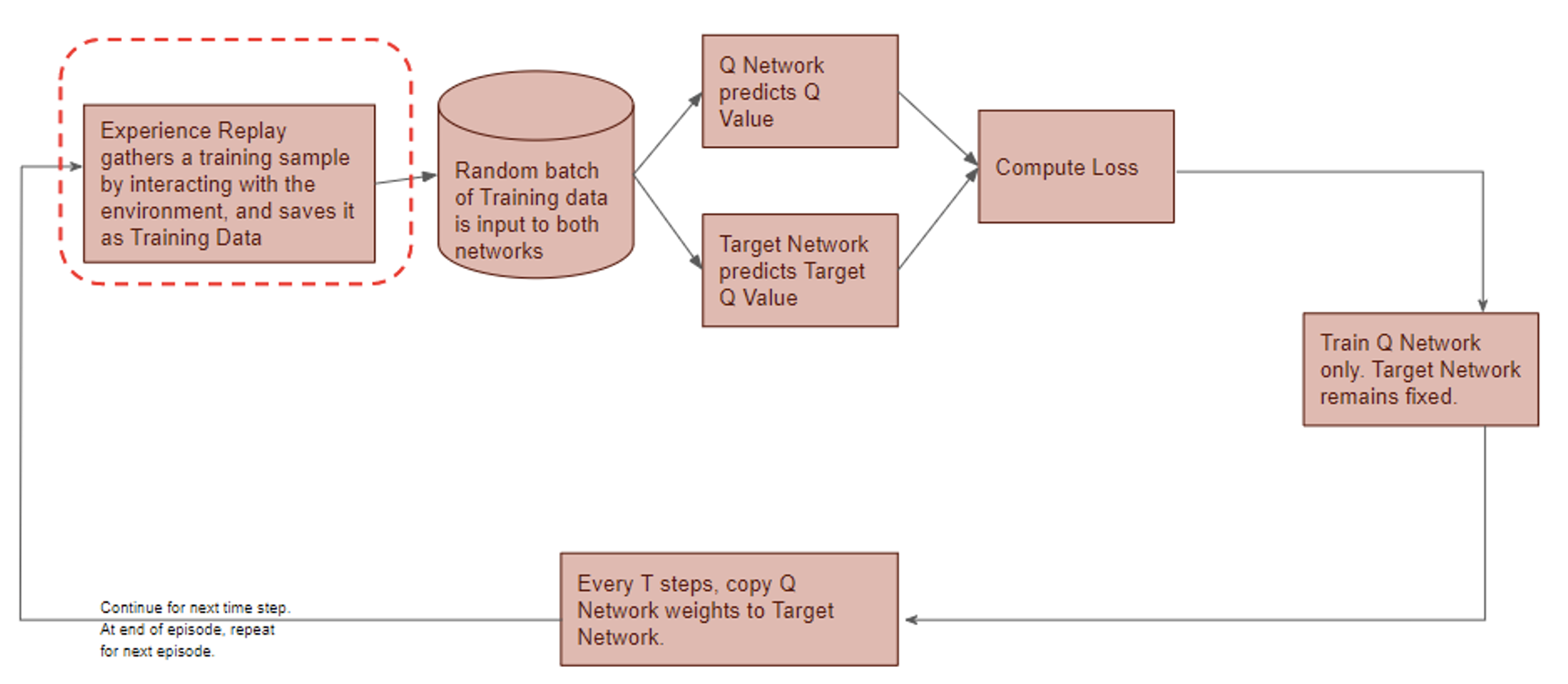
1) Experience replay selects an action according to the behavior policy, executes in the environment, returns the reward and next state. This experience set (\phi_t, a_t, r_r,\phi_{t+!}) is stored in the repository as a sample of training data.

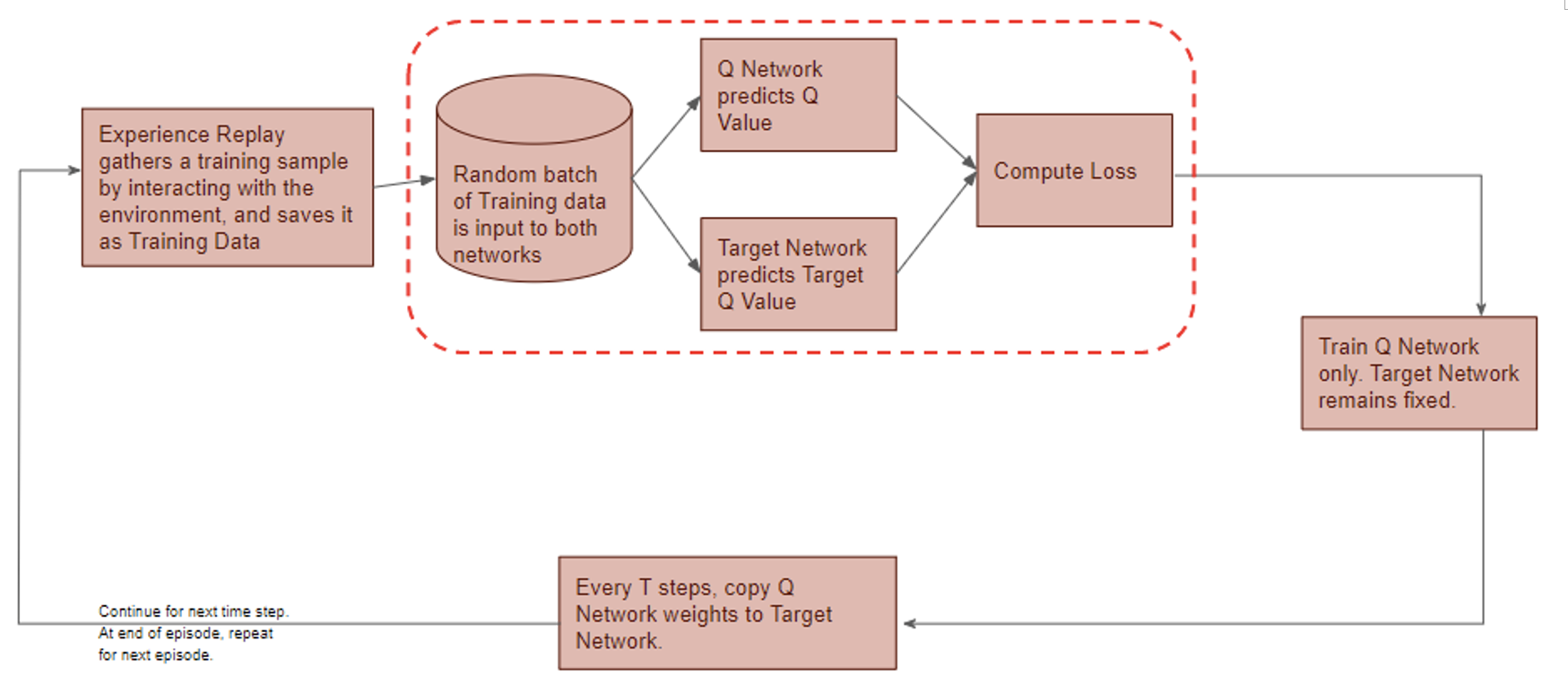
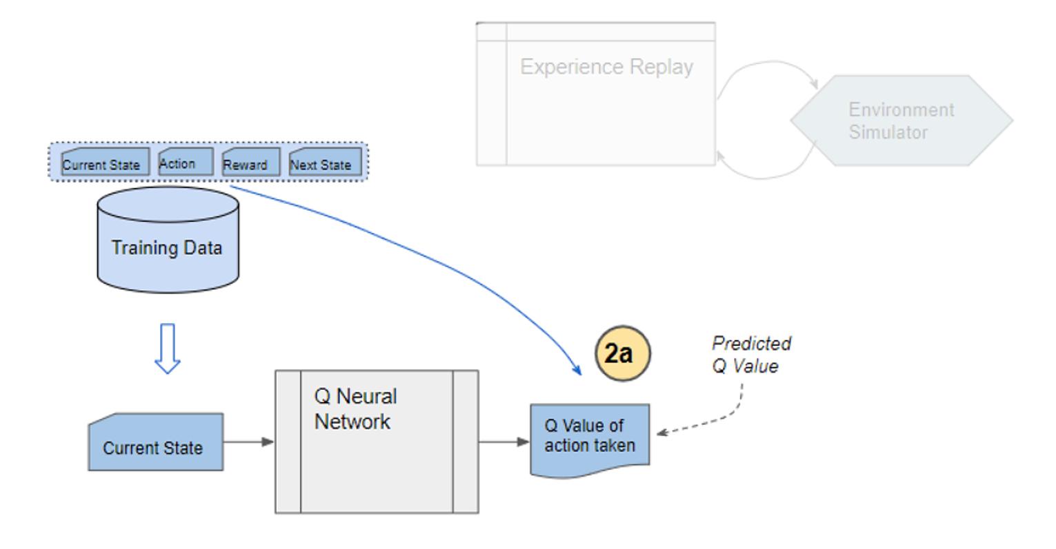
2) From the repository of prior observations, take a random batch of samples as the input to both Q- and Target network. The Q-network takes the current state and action from each data sample and predicts the q-value for that particular action. This is the ‘Predicted Q-Value’.Comment: Author uses 𝜀-greedy algorithm to calculate q-value and select action. To simplify, 𝜀-greedy policy takes the optimal action if a randomly generated number is greater than 𝜀, which represents a tradeoff between exploration and exploitation.

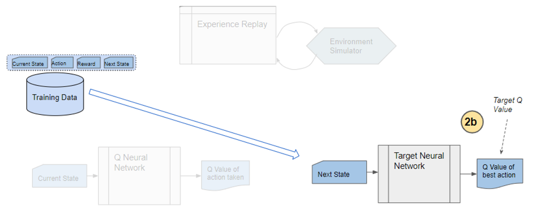
The Target network takes the next state from each data sample and predicts the best q-value out of all actions that can be taken from that state. This is the ‘Target Q-Value’.

Comment: Author proposes a different target policy to calculate the target q-value.

3) The Predicted q-value, Target q-value, and the observed reward from the data sample is used to compute the Loss to train the Q-network.

Comment: Target Network is not trained. It is held constant to serve as a stable target for learning and will be updated with a frequency different from the Q-network.

4) Copy Q-network weights to Target network after n time steps and continue to next time step until this episode is finished.

The architecutre of the proposed trading agent system.

4.0 Main Contribution of the Research

4.1 Action and Reward

Agent determines not only action a but ratio , at which the action is applied.

  1. Action:
    Hold, buy and sell. Buy and sell are defined discretely for each asset. Hold holds all assets. Therefore, there are (2m + 1) actions in the action set A.

    Agent obtains q-value of each action through q-network and selects action by using 𝜀-greedy algorithm as behavior policy.
  2. Ratio:
    \sigma is defined as the softmax value for the q-value of each action (ie. i-th asset at \sigma = 0.5 , then i-th asset is bought using 50% of base currency).
  3. Reward:
    Reward depends on the portfolio value before and after the trading strategy. It is clipped to [-1,1] to avoid overfitting.

4.2 Proposed Target Policy

Author sets the target based on the expected SARSA algorithm with some modification.

Comment: Author claims that greedy policy ignores the risks that may arise from exploring other outcomes other than the optimal one, which is fatal for domains where safe actions are preferred (ie. capital market).

The proposed policy uses softmax algorithm adjusted with greediness according to the temperature term 𝜏. However, softmax value is very sensitive to the differences in optimal q-value of states. To stabilize  learning, and thus to get similar greediness in all states, author redefine 𝜏 as the mean of absolute values for all q-values in each state multiplied by a hyperparameter 𝜏’.

4.3 Q-Network Structure

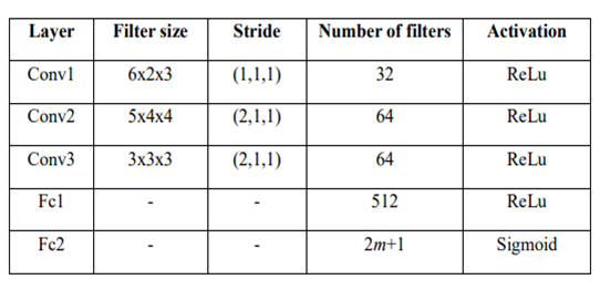
This study uses Convolutional Neural Network (CNN) to construct the networks. Detailed structure of the networks is shown in Table 2.

Comment: CNN is a deep neural network method that hierarchically extracts local features through a weighted filter. More details see: https://towardsdatascience.com/stock-market-action-prediction-with-convnet-8689238feae3.

5 Experiment and Hyperparameter Tuning

5.1 Experiment Setting

Data is collected from August 2017 to March 2018 when the price fluctuates extensively.

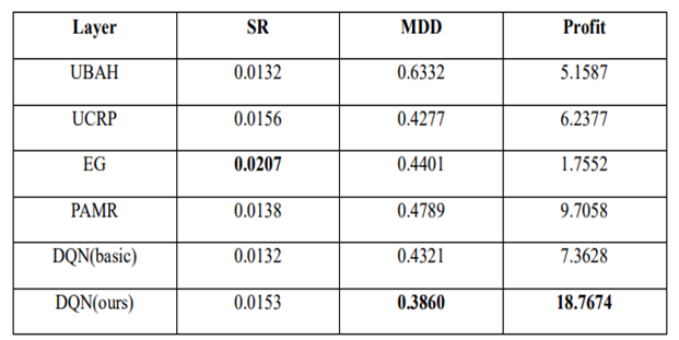
Three evaluation metrics are used to compare the performance of the trading agent.

  • Profit P_t introduced in 2.1.
  • Sharpe Ratio: A measure of return, taking risk into account.

    Comment: p_t is the standard deviation of the expected return and P_f  is the return of a risk-free asset, which is set to 0 here.
  • Maximum Drawdown: Maximum loss from a peak to a through, taking downside risk into account.

5.2 Hyperparameter Optimization

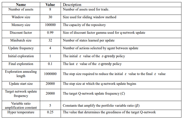
The proposed method has a number of hyperparameters: window size mentioned in 2.2,  𝜏’ in the target policy, and hyperparameters used in DQN structure. Author believes the former two are key determinants for the study and performs GridSearch to set w = 30, 𝜏’ = 0.25. The other hyperparameters are determined using heuristic search. Specifications of all hyperparameters are summarized in the last page.

Comment: Heuristic is a type of search that looks for a good solution, not necessarily a perfect one, out of the available options.

5.3 Performance Evaluation

Benchmark algorithms:

UBAH (Uniform buy and hold): Invest in all assets and hold until the end.
UCRP (Uniform Constant Rebalanced Portfolio): Rebalance portfolio uniformly for every trading period.

Methods from other studies: hyperparameters as suggested in the studies
EG (Exponential Gradient)
PAMR (Passive Aggressive Mean Reversion Strategy)

Comment: DQN basic uses greedy policy as the target policy.

The proposed DQN method exhibits the best overall results out of the 6 methods. When the agent is trained with shorter periods, although MDD increases significantly, it still performs better than benchmarks and proves its robustness.

6 Conclusion

The proposed method performs well compared to other methods, but there is a main drawback. The encoding method lacked a theoretical basis to successfully encode the information in the capital market, and this opaqueness is a rooted problem for deep learning. Second, the study focuses on its target policy, while there remains room for improvement with its neural network structure.

Specification of Hyperparameters

Specification of Hyperparameters.


References

  1. Shin, S. Bu and S. Cho, “Automatic Financial Trading Agent for Low-risk Portfolio Management using Deep Reinforcement Learning”, https://arxiv.org/pdf/1909.03278.pdf
  2. Li, P. Zhao, S. C. Hoi, and V. Gopalkrishnan, “PAMR: passive aggressive mean reversion strategy for portfolio selection,” Machine learning, vol. 87, pp. 221-258, 2012.
  3. P. Helmbold, R. E. Schapire, Y. Singer, and M. K. Warmuth, “On‐line portfolio selection using multiplicative updates,” Mathematical Finance, vol. 8, pp. 325-347, 1998.

https://deepai.org/machine-learning-glossary-and-terms/softmax-layer#:~:text=The%20softmax%20function%20is%20a,can%20be%20interpreted%20as%20probabilities.

http://www.kasimte.com/2020/02/14/how-does-temperature-affect-softmax-in-machine-learning.html

https://towardsdatascience.com/reinforcement-learning-made-simple-part-2-solution-approaches-7e37cbf2334e

https://towardsdatascience.com/reinforcement-learning-explained-visually-part-4-q-learning-step-by-step-b65efb731d3e

https://towardsdatascience.com/reinforcement-learning-explained-visually-part-3-model-free-solutions-step-by-step-c4bbb2b72dcf

https://towardsdatascience.com/reinforcement-learning-explained-visually-part-5-deep-q-networks-step-by-step-5a5317197f4b

Wie Maschinen uns verstehen: Natural Language Understanding

Foto von Sebastian Bill auf Unsplash.

Natural Language Understanding (NLU) ist ein Teilbereich von Computer Science, der sich damit beschäftigt natürliche Sprache, also beispielsweise Texte oder Sprachaufnahmen, verstehen und verarbeiten zu können. Das Ziel ist es, dass eine Maschine in der gleichen Weise mit Menschen kommunizieren kann, wie es Menschen untereinander bereits seit Jahrhunderten tun.

Was sind die Bereiche von NLU?

Eine neue Sprache zu erlernen ist auch für uns Menschen nicht einfach und erfordert viel Zeit und Durchhaltevermögen. Wenn eine Maschine natürliche Sprache erlernen will, ist es nicht anders. Deshalb haben sich einige Teilbereiche innerhalb des Natural Language Understandings herausgebildet, die notwendig sind, damit Sprache komplett verstanden werden kann.

Diese Unterteilungen können auch unabhängig voneinander genutzt werden, um einzelne Aufgaben zu lösen:

  • Speech Recognition versucht aufgezeichnete Sprache zu verstehen und in textuelle Informationen umzuwandeln. Das macht es für nachgeschaltete Algorithmen einfacher die Sprache zu verarbeiten. Speech Recognition kann jedoch auch alleinstehend genutzt werden, beispielsweise um Diktate oder Vorlesungen in Text zu verwandeln.
  • Part of Speech Tagging wird genutzt, um die grammatikalische Zusammensetzung eines Satzes zu erkennen und die einzelnen Satzbestandteile zu markieren.
  • Named Entity Recognition versucht innerhalb eines Textes Wörter und Satzbausteine zu finden, die einer vordefinierten Klasse zugeordnet werden können. So können dann zum Beispiel alle Phrasen in einem Textabschnitt markiert werden, die einen Personennamen enthalten oder eine Zeit ausdrücken.
  • Sentiment Analysis klassifiziert das Sentiment, also die Gefühlslage, eines Textes in verschiedene Stufen. Dadurch kann beispielsweise automatisiert erkannt werden, ob eine Produktbewertung eher positiv oder eher negativ ist.
  • Natural Language Generation ist eine allgemeine Gruppe von Anwendungen mithilfe derer automatisiert neue Texte generiert werden sollen, die möglichst natürlich klingen. Zum Beispiel können mithilfe von kurzen Produkttexten ganze Marketingbeschreibungen dieses Produkts erstellt werden.

Welche Algorithmen nutzt man für NLP?

Die meisten, grundlegenden Anwendungen von NLP können mit den Python Modulen spaCy und NLTK umgesetzt werden. Diese Bibliotheken bieten weitreichende Modelle zur direkten Anwendung auf einen Text, ohne vorheriges Trainieren eines eigenen Algorithmus. Mit diesen Modulen ist ohne weiteres ein Part of Speech Tagging oder Named Entity Recognition in verschiedenen Sprachen möglich.

Der Hauptunterschied zwischen diesen beiden Bibliotheken ist die Ausrichtung. NLTK ist vor allem für Entwickler gedacht, die eine funktionierende Applikation mit Natural Language Processing Modulen erstellen wollen und dabei auf Performance und Interkompatibilität angewiesen sind. SpaCy hingegen versucht immer Funktionen bereitzustellen, die auf dem neuesten Stand der Literatur sind und macht dabei möglicherweise Einbußen bei der Performance.

Für umfangreichere und komplexere Anwendungen reichen jedoch diese Optionen nicht mehr aus, beispielsweise wenn man eine eigene Sentiment Analyse erstellen will. Je nach Anwendungsfall sind dafür noch allgemeine Machine Learning Modelle ausreichend, wie beispielsweise ein Convolutional Neural Network (CNN). Mithilfe von Tokenizern von spaCy oder NLTK können die einzelnen in Wörter in Zahlen umgewandelt werden, mit denen wiederum das CNN als Input arbeiten kann. Auf heutigen Computern sind solche Modelle mit kleinen Neuronalen Netzwerken noch schnell trainierbar und deren Einsatz sollte deshalb immer erst geprüft und möglicherweise auch getestet werden.

Jedoch gibt es auch Fälle in denen sogenannte Transformer Modelle benötigt werden, die im Bereich des Natural Language Processing aktuell state-of-the-art sind. Sie können inhaltliche Zusammenhänge in Texten besonders gut mit in die Aufgabe einbeziehen und liefern daher bessere Ergebnisse beispielsweise bei der Machine Translation oder bei Natural Language Generation. Jedoch sind diese Modelle sehr rechenintensiv und führen zu einer sehr langen Rechenzeit auf normalen Computern.

Was sind Transformer Modelle?

In der heutigen Machine Learning Literatur führt kein Weg mehr an Transformer Modellen aus dem Paper „Attention is all you need“ (Vaswani et al. (2017)) vorbei. Speziell im Bereich des Natural Language Processing sind die darin erstmals beschriebenen Transformer Modelle nicht mehr wegzudenken.

Transformer werden aktuell vor allem für Übersetzungsaufgaben genutzt, wie beispielsweise auch bei www.deepl.com. Darüber hinaus sind diese Modelle auch für weitere Anwendungsfälle innerhalb des Natural Language Understandings geeignet, wie bspw. das Beantworten von Fragen, Textzusammenfassung oder das Klassifizieren von Texten. Das GPT-2 Modell ist eine Implementierung von Transformern, dessen Anwendungen und die Ergebnisse man hier ausprobieren kann.

Was macht den Transformer so viel besser?

Soweit wir wissen, ist der Transformer jedoch das erste Transduktionsmodell, das sich ausschließlich auf die Selbstaufmerksamkeit (im Englischen: Self-Attention) stützt, um Repräsentationen seiner Eingabe und Ausgabe zu berechnen, ohne sequenzorientierte RNNs oder Faltung (im Englischen Convolution) zu verwenden.

Übersetzt aus dem englischen Originaltext: Attention is all you need (Vaswani et al. (2017)).

In verständlichem Deutsch bedeutet dies, dass das Transformer Modell die sogenannte Self-Attention nutzt, um für jedes Wort innerhalb eines Satzes die Beziehung zu den anderen Wörtern im gleichen Satz herauszufinden. Dafür müssen nicht, wie bisher, Recurrent Neural Networks oder Convolutional Neural Networks zum Einsatz kommen.

Was dieser Mechanismus konkret bewirkt und warum er so viel besser ist, als die vorherigen Ansätze wird im folgenden Beispiel deutlich. Dazu soll der folgende deutsche Satz mithilfe von Machine Learning ins Englische übersetzt werden:

„Das Mädchen hat das Auto nicht gesehen, weil es zu müde war.“

Für einen Computer ist diese Aufgabe leider nicht so einfach, wie für uns Menschen. Die Schwierigkeit an diesem Satz ist das kleine Wort „es“, dass theoretisch für das Mädchen oder das Auto stehen könnte. Aus dem Kontext wird jedoch deutlich, dass das Mädchen gemeint ist. Und hier ist der Knackpunkt: der Kontext. Wie programmieren wir einen Algorithmus, der den Kontext einer Sequenz versteht?

Vor Veröffentlichung des Papers „Attention is all you need“ waren sogenannte Recurrent Neural Networks die state-of-the-art Technologie für solche Fragestellungen. Diese Netzwerke verarbeiten Wort für Wort eines Satzes. Bis man also bei dem Wort „es“ angekommen ist, müssen erst alle vorherigen Wörter verarbeitet worden sein. Dies führt dazu, dass nur noch wenig Information des Wortes „Mädchen“ im Netzwerk vorhanden sind bis den Algorithmus überhaupt bei dem Wort „es“ angekommen ist. Die vorhergegangenen Worte „weil“ und „gesehen“ sind zu diesem Zeitpunkt noch deutlich stärker im Bewusstsein des Algorithmus. Es besteht also das Problem, dass Abhängigkeiten innerhalb eines Satzes verloren gehen, wenn sie sehr weit auseinander liegen.

Was machen Transformer Modelle anders? Diese Algorithmen prozessieren den kompletten Satz gleichzeitig und gehen nicht Wort für Wort vor. Sobald der Algorithmus das Wort „es“ in unserem Beispiel übersetzen will, wird zuerst die sogenannte Self-Attention Layer durchlaufen. Diese hilft dem Programm andere Wörter innerhalb des Satzes zu erkennen, die helfen könnten das Wort „es“ zu übersetzen. In unserem Beispiel werden die meisten Wörter innerhalb des Satzes einen niedrigen Wert für die Attention haben und das Wort Mädchen einen hohen Wert. Dadurch ist der Kontext des Satzes bei der Übersetzung erhalten geblieben.

Big Data mit Hadoop und Map Reduce!

Foto von delfi de la Rua auf Unsplash.

Hadoop ist ein Softwareframework, mit dem sich große Datenmengen auf verteilten Systemen schnell verarbeiten lassen. Es verfügt über Mechanismen, welche eine stabile und fehlertolerante Funktionalität sicherstellen, sodass das Tool für die Datenverarbeitung im Big Data Umfeld bestens geeignet ist. In diesen Fällen ist eine normale relationale Datenbank oft nicht ausreichend, um die unstrukturierten Datenmengen kostengünstig und effizient abzuspeichern.

Unterschiede zwischen Hadoop und einer relationalen Datenbank

Hadoop unterscheidet sich in einigen grundlegenden Eigenschaften von einer vergleichbaren relationalen Datenbank.

Eigenschaft Relationale Datenbank Hadoop
Datentypen ausschließlich strukturierte Daten alle Datentypen (strukturiert, semi-strukturiert und unstrukturiert)
Datenmenge wenig bis mittel (im Bereich von einigen GB) große Datenmengen (im Bereich von Terrabyte oder Petabyte)
Abfragesprache SQL HQL (Hive Query Language)
Schema Statisches Schema (Schema on Write) Dynamisches Schema (Schema on Read)
Kosten Lizenzkosten je nach Datenbank Kostenlos
Datenobjekte Relationale Tabellen Key-Value Pair
Skalierungstyp Vertikale Skalierung (Computer muss hardwaretechnisch besser werden) Horizontale Skalierung (mehr Computer können dazugeschaltet werden, um Last abzufangen)

Vergleich Hadoop und Relationale Datenbank

Bestandteile von Hadoop

Das Softwareframework selbst ist eine Zusammenstellung aus insgesamt vier Komponenten.

Hadoop Common ist eine Sammlung aus verschiedenen Modulen und Bibliotheken, welche die anderen Bestandteile unterstützt und deren Zusammenarbeit ermöglicht. Unter anderem sind hier die Java Archive Dateien (JAR Files) abgelegt, die zum Starten von Hadoop benötigt werden. Darüber hinaus ermöglicht die Sammlung die Bereitstellung von grundlegenden Services, wie beispielsweise das File System.

Der Map-Reduce Algorithmus geht in seinen Ursprüngen auf Google zurück und hilft komplexe Rechenaufgaben in überschaubarere Teilprozesse aufzuteilen und diese dann über mehrere Systeme zu verteilen, also horizontal zu skalieren. Dadurch verringert sich die Rechenzeit deutlich. Am Ende müssen die Ergebnisse der Teilaufgaben wieder zu seinem Gesamtresultat zusammengefügt werden.

Der Yet Another Resource Negotiator (YARN) unterstützt den Map-Reduce Algorithmus, indem er die Ressourcen innerhalb eines Computer Clusters im Auge behält und die Teilaufgaben auf die einzelnen Rechner verteilt. Darüber hinaus ordnet er den einzelnen Prozessen die Kapazitäten dafür zu.

Das Hadoop Distributed File System (HDFS) ist ein skalierbares Dateisystem zur Speicherung von Zwischen- oder Endergebnissen. Innerhalb des Clusters ist es über mehrere Rechner verteilt, um große Datenmengen schnell und effizient verarbeiten zu können. Die Idee dahinter war, dass Big Data Projekte und Datenanalysen auf großen Datenmengen beruhen. Somit sollte es ein System geben, welches die Daten auch stapelweise speichert und dadurch schnell verarbeitet. Das HDFS sorgt auch dafür, dass Duplikate von Datensätzen abgelegt werden, um den Ausfall eines Rechners verkraften zu können.

Map Reduce am Beispiel

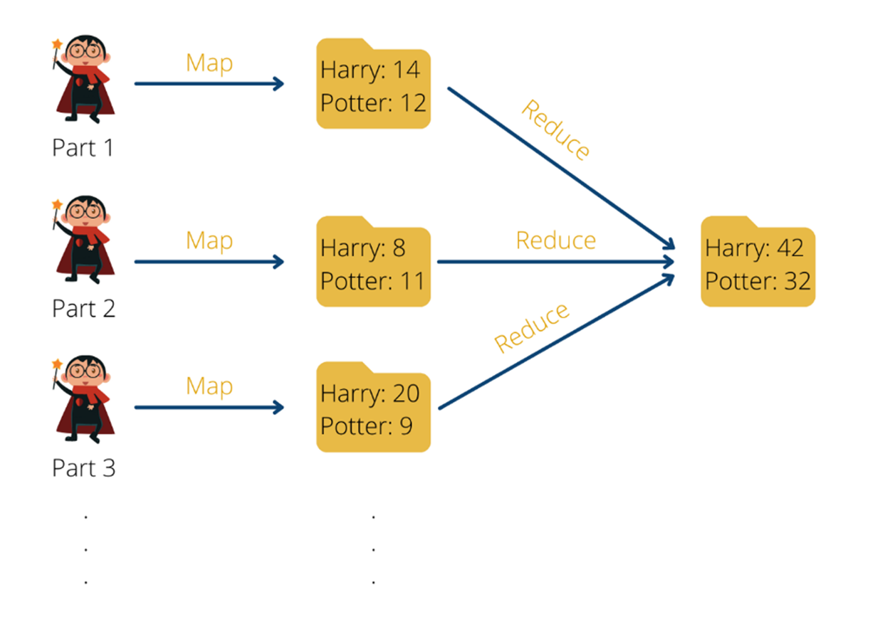
Angenommen wir haben alle Teile der Harry Potter Romane in Hadoop PDF abgelegt und möchten nun die einzelnen Wörter zählen, die in den Büchern vorkommen. Dies ist eine klassische Aufgabe bei der uns die Aufteilung in eine Map-Funktion und eine Reduce Funktion helfen kann.

Bevor es die Möglichkeit gab, solche aufwendigen Abfragen auf ein ganzes Computer-Cluster aufzuteilen und parallel berechnen zu können, war man gezwungen, den kompletten Datensatz nacheinander zu durchlaufen. Dadurch wurde die Abfragezeit auch umso länger, umso größer der Datensatz wurde. Der einzige Weg, um die Ausführung der Funktion zu beschleunigen ist es, einen Computer mit einem leistungsfähigeren Prozessor (CPU) auszustatten, also dessen Hardware zu verbessern. Wenn man versucht, die Ausführung eines Algorithmus zu beschleunigen, indem man die Hardware des Gerätes verbessert, nennt man das vertikale Skalieren.

Mithilfe von MapReduce ist es möglich eine solche Abfrage deutlich zu beschleunigen, indem man die Aufgabe in kleinere Teilaufgaben aufsplittet. Das hat dann wiederum den Vorteil, dass die Teilaufgaben auf viele verschiedene Computer aufgeteilt und von ihnen ausgeführt werden kann. Dadurch müssen wir nicht die Hardware eines einzigen Gerätes verbessern, sondern können viele, vergleichsweise leistungsschwächere, Computer nutzen und trotzdem die Abfragezeit verringern. Ein solches Vorgehen nennt man horizontales Skalieren.

Kommen wir zurück zu unserem Beispiel: Bisher waren wir bildlich so vorgegangen, dass wir alle Harry Potter Teile gelesen haben und nach jedem gelesenen Wort die Strichliste mit den einzelnen Wörtern einfach um einen Strich erweitert haben. Das Problem daran ist, dass wir diese Vorgehensweise nicht parallelisieren können. Angenommen eine zweite Person will uns unterstützen, dann kann sie das nicht tun, weil sie die Strichliste, mit der wir gerade arbeiten, benötigt, um weiterzumachen. Solange sie diese nicht hat, kann sie nicht unterstützen.

Sie kann uns aber unterstützen, indem sie bereits mit dem zweiten Teil der Harry Potter Reihe beginnt und eine eigene Strichliste nur für das zweite Buch erstellt. Zum Schluss können wir dann alle einzelnen Strichlisten zusammenführen und beispielsweise die Häufigkeit des Wortes “Harry” auf allen Strichlisten zusammenaddieren.

MapReduce am Beispiel von Wortzählungen in Harry Potter Büchern

MapReduce am Beispiel von Wortzählungen in Harry Potter Büchern | Source: Data Basecamp

Dadurch lässt sich die Aufgabe auch relativ einfach horizontal skalieren, indem jeweils eine Person pro Harry Potter Buch arbeitet. Wenn wir noch schneller arbeiten wollen, können wir auch mehrere Personen mit einbeziehen und jede Person ein einziges Kapitel bearbeiten lassen. Am Schluss müssen wir dann nur alle Ergebnisse der einzelnen Personen zusammennehmen, um so zu einem Gesamtergebnis zu gelangen.

Das ausführliche Beispiel und die Umsetzung in Python findest Du hier.

Aufbau eines Hadoop Distributed File Systems

Der Kern des Hadoop Distributed File Systems besteht darin die Daten auf verschiedene Dateien und Computer zu verteilen, sodass Abfragen schnell bearbeitet werden können und der Nutzer keine langen Wartezeiten hat. Damit der Ausfall einer einzelnen Maschine im Cluster nicht zum Verlust der Daten führt, gibt es gezielte Replikationen auf verschiedenen Computern, um eine Ausfallsicherheit zu gewährleisten.

Hadoop arbeitet im Allgemeinen nach dem sogenannten Master-Slave-Prinzip. Innerhalb des Computerclusters haben wir einen Knoten, der die Rolle des sogenannten Masters übernimmt. Dieser führt in unserem Beispiel keine direkte Berechnung durch, sondern verteilt lediglich die Aufgaben auf die sogenannten Slave Knoten und koordiniert den ganzen Prozess. Die Slave Knoten wiederum lesen die Bücher aus und speichern die Worthäufigkeit und die Wortverteilung.

Dieses Prinzip wird auch bei der Datenspeicherung genutzt. Der Master verteilt Informationen aus dem Datensatz auf verschiedenen Slave Nodes und merkt sich, auf welchen Computern er welche Partitionen abgespeichert hat. Dabei legt er die Daten auch redundant ab, um Ausfälle kompensieren zu können. Bei einer Abfrage der Daten durch den Nutzer entscheidet der Masterknoten dann, welche Slaveknoten er anfragen muss, um die gewünschten Informationen zu erhalten.

Automated product quality monitoring using artificial intelligence deep learning

How to maintain product quality with deep learning

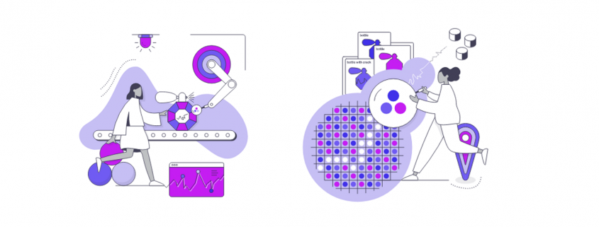
Deep Learning helps companies to automate operative processes in many areas. Industrial companies in particular also benefit from product quality assurance by automated failure and defect detection. Computer Vision enables automation to identify scratches and cracks on product item surfaces. You will find more information about how this works in the following infografic from DATANOMIQ and pixolution you can download using the link below.

How to maintain product quality with automatic defect detection - Infographic

How to maintain product quality with automatic defect detection – Infographic

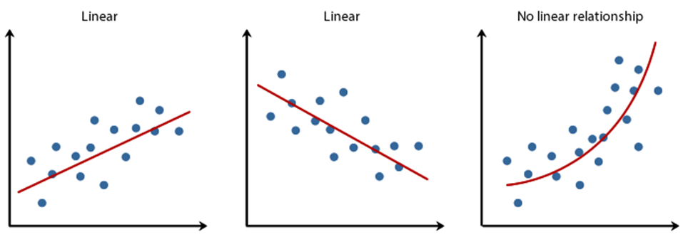
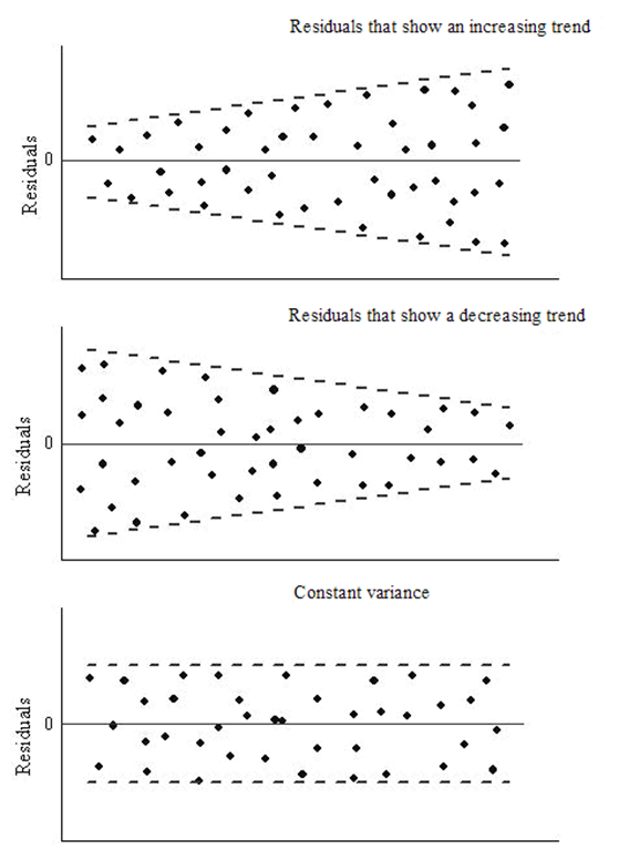
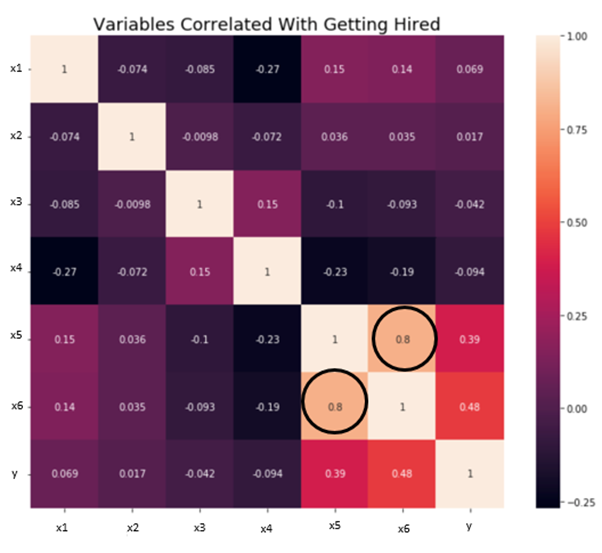
Understanding Linear Regression with all Statistical Terms

Linear Regression Model – This article is about understanding the linear regression with all the statistical terms.

What is Regression Analysis?

regression is an attempt to determine the relationship between one dependent and a series of other independent variables.

Regression analysis is a form of predictive modelling technique which investigates the relationship between a dependent (target) and independent variable (s) (predictor). This technique is used for forecasting, time series modelling and finding the causal effect relationship between the variables. For example, relationship between rash driving and number of road accidents by a driver is best studied through regression.

Why do we use Regression Analysis?

As mentioned above, regression analysis estimates the relationship between two or more variables. Let’s understand this with an easy example:

Let’s say, you want to estimate growth in sales of a company based on current economic conditions. You have the recent company data which indicates that the growth in sales is around two and a half times the growth in the economy. Using this insight, we can predict future sales of the company based on current & past information.

There are multiple benefits of using regression analysis. They are as follows:

It indicates the significant relationships between dependent variable and independent variable. It indicates the strength of impact of multiple independent variables on a dependent variable. Regression analysis also allows us to compare the effects of variables measured on different scales, such as the effect of price changes and the number of promotional activities. These benefits help market researchers / data analysts / data scientists to eliminate and evaluate the best set of variables to be used for building predictive models.

There are various kinds of regression techniques available to make predictions. These techniques are mostly driven by three metrics (number of independent variables, type of dependent variables and shape of regression line).

Number of independent variables, shape of regression line and type of dependent variable.

Number of independent variables, shape of regression line and type of dependent variable.

What is Linear Regression?

Linear Regression is the supervised Machine Learning model in which the model finds the best fit linear line between the independent and dependent variable i.e it finds the linear relationship between the dependent and independent variable.

  • Equation of Simple Linear Regression, where bo is the intercept, b1 is coefficient or slope, x is the independent variable and y is the dependent variable.

Equation of Multiple Linear Regression, where bo is the intercept, b1,b2,b3,b4…,bn are coefficients or slopes of the independent variables x1,x2,x3,x4…,xn and y is the y=b_0+b_1x_1+b_2x_2+…+b_nx_n dependent variable.

Linear regression and its error termin per value

Linear regression and its error termin per value

Mathematical Approach:

Residual/Error = Actual values – Predicted Values
Sum of Residuals/Errors = Sum(Actual- Predicted Values)
Square of Sum of Residuals/Errors = (Sum(Actual- Predicted Values))^2

\sum(e_i^2)=\sum(y_i-\hat{y_i})^2

Application of Linear Regression:

Real-world examples of linear regression models
  1. Businesses often use linear regression to understand the relationship between advertising spending and revenue.
  2. Medical researchers often use linear regression to understand the relationship between drug dosage and blood pressure of patients.
  3. Agricultural scientists often use linear regression to measure the effect of fertilizer and water on crop yields.
  4. Data scientists for professional sports teams often use linear regression to measure the effect that different training regimens have on player performance.
  5. Stock predictions: A lot of businesses use linear regression models to predict how stocks will perform in the future. This is done by analyzing past data on stock prices and trends to identify patterns.
  6. Predicting consumer behavior: Businesses can use linear regression to predict things like how much a customer is likely to spend. Regression models can also be used to predict consumer behavior. This can be helpful for things like targeted marketing and product development. For example, Walmart uses linear regression to predict what products will be popular in different regions of the country.

Assumptions of Linear Regression:

Linearity: It states that the dependent variable Y should be linearly related to independent variables. This assumption can be checked by plotting a scatter plot between both variables.

Normality: The X and Y variables should be normally distributed. Histograms, KDE plots, Q-Q plots can be used to check the Normality assumption.

Homoscedasticity: The variance of the error terms should be constant i.e the spread of residuals should be constant for all values of X. This assumption can be checked by plotting a residual plot. If the assumption is violated then the points will form a funnel shape otherwise they will be constant.

Independence/No Multicollinearity: The variables should be independent of each other i.e no correlation should be there between the independent variables. To check the assumption, we can use a correlation matrix or VIF score. If the VIF score is greater than 5 then the variables are highly correlated.

The error terms should be normally distributed. Q-Q plots and Histograms can be used to check the distribution of error terms.

No Autocorrelation: The error terms should be independent of each other. Autocorrelation can be tested using the Durbin Watson test. The null hypothesis assumes that there is no autocorrelation. The value of the test lies between 0 to 4. If the value of the test is 2 then there is no autocorrelation.