Data Science Hack Archives

Continuous Integration and Continuous Delivery (CI/CD) for Data Pipelines

The Crucial Intersection of Generative AI and Data Quality: Ensuring Reliable Insights

October 1, 2024/in Artificial Intelligence, Big Data, Business Analytics, Business Intelligence, Data Engineering, Data Science, Deep Learning, Main Category, Tools/by AnalyticsCreator

In data analytics, data’s quality is the bedrock of reliable insights. Just like a skyscraper’s stability depends on a solid foundation, the accuracy and reliability of your insights rely on top-notch data quality. Enter Generative AI – a game-changing technology revolutionizing data management and utilization. Combined with strict data quality practices, Generative AI becomes an incredibly powerful tool, enabling businesses to extract actionable and trustworthy insights.

Building the Foundation: Data Quality

Data quality is the foundation of all analytical endeavors. Poor data quality can lead to faulty analyses, misguided decisions, and ultimately, a collapse in trust. Businesses must ensure their data is clean, structured, and reliable. Without this, even the most sophisticated AI algorithms will produce skewed results.

Generative AI: The Master Craftsman

Generative AI, with its ability to create, predict, and optimize data patterns, refines raw data into valuable insights, automates repetitive tasks, and identifies hidden patterns that might elude human analysts. However, for this to work effectively, it requires high-quality raw materials – that is, impeccable data.

Imagine Generative AI as an artist creating a detailed painting. If the artist is provided with subpar paint and brushes, the resulting artwork will be flawed. Conversely, with high-quality tools, the artist can produce a masterpiece. Similarly, Generative AI needs high-quality data to generate reliable and actionable insights.

The Symbiotic Relationship

The relationship between data quality and Generative AI is symbiotic. High-quality data enhances the performance of Generative AI, while Generative AI can improve data quality through advanced data cleaning, anomaly detection, and data augmentation techniques.

For instance, Generative AI can identify and rectify inconsistencies in datasets, fill in missing values with remarkable accuracy, and generate synthetic data to enhance training datasets for machine learning models. This creates a virtuous cycle where improved data quality leads to better AI performance, which further refines data quality.

Practical Steps for Businesses

Assess Data Quality Regularly: Implement robust data quality assessment frameworks to continuously monitor and improve the quality of your data.
Leverage AI for Data Management: Utilize Generative AI tools to automate data cleaning, error detection, and data augmentation processes.
Invest in Training and Tools: Ensure your team is equipped with the necessary skills and tools to manage and utilize Generative AI effectively.
Foster a Data-Driven Culture: Encourage a culture where data quality is prioritized, and insights are derived from reliable, high-quality data sources.

The AnalyticsCreator Advantage

AnalyticsCreator stands at the forefront of this intersection, offering solutions that seamlessly integrate data quality measures with Generative AI capabilities. By partnering with AnalyticsCreator, businesses can ensure that their analytical foundations are solid, with Generative AI sculpting insights that drive informed decision-making.

In the rapidly evolving landscape of data analytics, the intersection of Generative AI and data quality is transformative. Ensuring high data quality while leveraging the power of Generative AI can propel businesses to new heights of efficiency and insight.

By embracing this symbiotic relationship, organizations can unlock the full potential of their data, paving the way for innovations and strategic advantages that are both reliable and groundbreaking. AnalyticsCreator is here to guide you through this journey, ensuring your data’s foundation is as strong as your vision for the future.

Looking Ahead: The Future of Data Preparation for Generative AI

August 22, 2024/in Business Analytics, Business Intelligence, Data Engineering, Data Migration, Data Warehousing, Main Category, Sponsoring Partner Posts, Tools/by AnalyticsCreator

Why using Infrastructure as Code for developing Cloud-based Data Warehouse Systems?

September 20, 2023/in Cloud, Data Engineering, Infrastructure as Code, Main Category, Tutorial/by Benjamin Aunkofer

In the contemporary age of Big Data, Data Warehouse Systems and Data Science Analytics Infrastructures have become an essential component for organizations to store, analyze, and make data-driven decisions. With the evolution of cloud computing, many organizations are now migrating their Data Warehouse Systems to the cloud for better scalability, flexibility, and cost-efficiency. Infrastructure as Code (IaC) can be a game-changer in this scenario. By automating the provisioning and management of cloud resources through code, IaC brings a host of advantages to the development and maintenance of Data Warehouse Systems in the cloud.

So why using IaC for Cloud Data Infrastructures?

Of course you – as a human user – can always login into the admin portal of any cloud provider and manually get your resources like SQL databases, ETL tools, Virtual Networks and tools like Synapse, snowflake, BigQuery or Databrikcs in place by clicking on the right buttons….. But here is why you should better follow the idea of having your code explaining which resources are in what order in place in your cloud:

Version Control for your Cloud Infrastructure

One of the primary advantages of using IaC is version control for your Data Warehouse – or Data Lakehouse – Architecture. Whether you’re using Redshift, Snowflake, or any other cloud-based data warehouse solutions, you can codify your architecture settings, allowing you to track changes over time. This ensures a reliable and consistent development environment and makes it easier to identify issues, rollback updates, or replicate the architecture for other projects.

Scalability Tailored for Data Needs

Data Warehouse Systems often require to scale quickly to handle larger datasets or more queries. Traditional manual scaling methods are cumbersome and slow. IaC allows for efficient auto-scaling based on real-time needs. You can write scripts to automatically provision or de-provision resources depending on your data workloads, making your data warehouse highly adaptive to your organization’s changing requirements.

Cost-Efficiency in Resource Allocation

Cloud resources are priced based on usage, so efficient allocation is crucial for managing costs. IaC enables precise control over cloud resources, allowing you to turn them off when not in use or allocate more resources during peak times. For Data Warehouse Systems that often require powerful (and expensive) computing resources, this level of control can translate into significant cost savings.

Streamlined Collaboration Among Teams

Data Warehouse Systems in the cloud often involve cross-functional teams — data engineers, data scientists, and system administrators. IaC allows these teams to collaborate more effectively. Everyone works with the same infrastructure configurations, reducing discrepancies between development, staging, and production environments. This ensures that the data models and queries developed by data professionals are consistent with the underlying infrastructure.

Enhanced Security and Compliance

Data Warehouses often store sensitive information, making security a paramount concern. IaC allows security configurations to be codified and automated, ensuring that every new resource or service deployed complies with organizational and regulatory guidelines. This proactive security approach is particularly beneficial for industries that have to adhere to strict compliance rules like HIPAA or GDPR.

Reliable Environment for Data Operations

Manual configurations are prone to human error, which can compromise the reliability of a Data Warehouse System. IaC mitigates this risk by automating repetitive tasks, ensuring that the infrastructure is consistently provisioned. This brings reliability to data ETL (Extract, Transform, Load) processes, query performances, and other critical data operations.

Documentation and Disaster Recovery Made Easy

Data is the lifeblood of any organization, and losing it can be catastrophic. IaC allows for swift disaster recovery by codifying the entire infrastructure. If a disaster occurs, the infrastructure can be quickly recreated, reducing downtime and data loss.

Most common IaC solutions

The most common tools for creating Cloud Infrastructure as Code are probably Terraform and Pulumi. However, IaC solutions can be very different in their concepts. For example: While Terraform is a pure declarative configuration language that just describes how the infrastructure will look like (execution then by the Terraform-supporting Cloud Provider), Pulumi on the other hand will execute the deployment by a programming language iteratively deploying the wished cloud resources (e.g. using for loops in Python). While executing Pulumi in any supported programming language like Python or C#, Pulumi generates declarative Infrastructure build plans for the Cloud. Any IaC solution is declaring how the infrastrcture looks like.

Terraform

Terraform is one of the most widely used Infrastructure as Code (IaC) tools, developed by HashiCorp. It enables users to define and provision a data center infrastructure using a declarative configuration language known as HashiCorp Configuration Language (HCL).

The following Terraform script will create an Azure Resource Group, a SQL Server, and a SQL Database. It will also output the fully qualified domain name (FQDN) of the SQL Server, which you can use to connect to the database:

provider "azurerm" {

features {}

}

resource "azurerm_resource_group" "example" {

name = "example-resources"

location = "East US"

}

resource "azurerm_sql_server" "example" {

name = "example-sqlserver"

resource_group_name = azurerm_resource_group.example.name

location = azurerm_resource_group.example.location

version = "12.0"

administrator_login = "adminUser"

administrator_login_password = "adminPassword1234!"

}

resource "azurerm_sql_database" "example" {

name = "example-sqldb"

resource_group_name = azurerm_resource_group.example.name

server_name = azurerm_sql_server.example.name

location = azurerm_resource_group.example.location

edition = "Basic"

}

output "sql_server_fqdn" {

value = azurerm_sql_server.example.fully_qualified_domain_name

}

The HCL code needs to be placed into the Terrafirm main.tf file. Of course, Terraform and the Azure CLI needs to be installed before.

Pulumi

Pulumi is a modern Infrastructure as Code (IaC) tool that sets itself apart by allowing infrastructure to be defined using general-purpose programming languages like Python, TypeScript, Go, and C#.

Example of a Pulumi Python script creating a SQL Database on Microsoft Azure Cloud:

import * as pulumi from "@pulumi/pulumi";

import * as azure from "@pulumi/azure";

// Create an Azure Resource Group

const resourceGroup = new azure.core.ResourceGroup("myResourceGroup", {

location: "EastUS",

});

// Create an Azure SQL Server

const sqlServer = new azure.sql.SqlServer("mySqlServer", {

resourceGroupName: resourceGroup.name,

location: resourceGroup.location,

version: "12.0",

administratorLogin: "adminUser",

administratorLoginPassword: "adminPassword1234!",

});

// Create an Azure SQL Database on the SQL Server

const sqlDatabase = new azure.sql.Database("mySqlDatabase", {

resourceGroupName: resourceGroup.name,

serverName: sqlServer.name,

location: resourceGroup.location,

edition: "Basic",

});

// Export connection string for the SQL Database

export const sqlConnectionString = pulumi.all([sqlServer.name, resourceGroup.name, sqlDatabase.name]).apply(([serverName, rgName, dbName]) => {

return `Server=tcp:${serverName}.database.windows.net;initial catalog=${dbName};user ID=adminUser;password=adminPassword1234!;Min Pool Size=0;Max Pool Size=30;Persist Security Info=true;`;

});

Running the script will need the installation of Python, Pulumi and the Azure CLI.

Cloud Provider specific IaC Solutions

Cloud providers might come up with their own IaC solutions, here are the probably most common ones:

Microsoft Azure Bicep is an open-source domain-specific language (DSL) developed by Microsoft, aimed at simplifying the process of deploying Azure resources. It serves as a declarative alternative to JSON for writing Azure Resource Manager (ARM) templates. Bicep compiles down to ARM templates, offering a more concise syntax and easier tooling while leveraging the proven, underlying ARM deployment engine.

AWS CloudFormation is a service offered by Amazon Web Services (AWS) that allows you to define cloud infrastructure in JSON or YAML templates.

Google Cloud Deployment Manager is quite similar to AWS CloudFormation but tailored for Google Cloud Platform (GCP), it allows you to define and deploy resources using YAML or Python templates.

IaC Tools for Server Configuration

There are many other IaC solutions and some of them are more focused on configuration of servers. In common they offer software provisioning as well and a lot detailing in regards to micro-configuration of single applications running on the server.

The most common IaC software for Server Configuration might be Ansible, a YAML-based configuration management tool that uses an agentless architecture. It’s easy to set up and widely used for automating tasks like software provisioning and configuration management. Puppet, Chef and SaltStack are further alternatives and master-agent architecture-based.

Conclusion

Infrastructure as Code significantly enhances the development and maintenance of Cloud-based Data Infrastructures. From versioning your warehouse architecture and scaling resources according to real-time data needs, to facilitating team collaboration and ensuring security compliance, IaC serves as a foundational technology that brings agility, reliability, and cost-efficiency. As organizations continue to realize the importance of data-driven decision-making, leveraging IaC for cloud-based Data Warehouse Systems will likely become a best practice in data engineering and infrastructure management.

Lambda Architecture vs Kappa Architecture for Big Data Cloud Platforms? Let us discuss which architecture suits best for what use cases.

Big Data – Lambda or Kappa Architecture?

June 27, 2023/in Big Data, Cloud, Cloud, Data Engineering, Main Category/by Benjamin Aunkofer

Big Data Analytics stands apart from conventional data processing in its fundamental nature. In the realm of Big Data, there are two prominent architectural concepts that perplex companies embarking on the construction or restructuring of their Big Data platform: Lambda architecture or Kappa architecture. Thus, it is crucial for such companies to contemplate and decide which architectural approach best aligns with their goals.

Lambda – Architecture

Introduced in 2011 during the peak of Big Data’s prominence, the Lambda architecture remains a significant presence in the field. Despite being the older of the two architectures, it offers a more comprehensive approach by incorporating three layers: the batch layer, the speed layer (also known as the stream layer), and the serving layer.

The Batch Layer is responsible for processing the entire dataset, ensuring the generation of the most accurate results. However, this comes at the cost of higher latency due to the batch loading of data. On the flip side, the batch layer can handle complex calculations without time constraints. It stores incoming raw data and filters it for subsequent applications.

Batch runs are suitable for non-time-sensitive data that require regular updates, such as daily or weekly incremental loads. Additionally, batch runs are necessary for complete data migration or overwriting (Full Load) scenarios.

The Speed Layer operates with low latency, producing almost real-time results. It calculates real-time views that complement the batch views. The speed layer receives incoming data and provides incremental updates to the batch layer results. By implementing incremental deduction logic, the speed layer significantly reduces computational costs.

Here is a simplified depiction of the Lambda architecture, showcasing the multi-store concept and the serving layer. In this representation, there is a separate store for events within the speed layer and another store for data loaded during batch processing. The serving layer acts as a mediator, enabling subsequent applications to access the data. It is important to note that in the Lambda architecture, the serving layer can be omitted, allowing batch processing and event streaming to remain separate entities.

The batch views within the Lambda architecture allow for the application of more complex or resource-intensive rules, resulting in superior data quality and reduced bias over time. On the other hand, the real-time views provide immediate access to the most current data.

The Serving Layer serves as a conduit for various data queries originating from both the batch and speed layers. It receives batch views from the batch layer and near-real-time views from the speed layer, utilizing this data to facilitate standard reporting and ad hoc analytics.

The Lambda architecture effectively balances speed, reliability, and scalability. However, it is worth mentioning that while the batch layer and real-time stream handle different scenarios, their underlying processing logic often shares similarities. As a result, the development and maintenance efforts for both layers should not be underestimated.

Kappa – Architecture

Jay Kreps introduced the Kappa architecture in 2014 as an alternative to the Lambda architecture. It addresses the redundancy present in the Lambda architecture by completely removing the batch component. By eliminating the parallel operation of two pipelines, the Kappa architecture simplifies the overall architectural complexity.

In the Kappa architecture, only the speed layer, represented by an event-based streaming pipeline, remains. The fundamental concept is to handle real-time data processing and continuous data reprocessing using a single stream processing engine. This approach allows for the avoidance of a multi-layer lambda architecture while ensuring the quality of data processing is maintained.

Illustrated simplified Kappa Architecture. This architectural concept relies on event streaming as the core element of data delivery.

In practical implementation, the Kappa architecture is commonly deployed using Apache Kafka or Kafka-based tools. Applications can directly read from and write to Kafka or an alternative message queue tool. For existing event sources, listeners are utilized to stream writes directly from database logs or similar data stores. This approach eliminates the need for inbound batch processing and reduces resource requirements.

By treating every data point as a streaming event, the Kappa architecture enables the ability to near-realtime analytics and observe the state of all data in the organization at any given point. Queries can be performed at a single location, eliminating the need to compare batch and velocity views.

However, there are challenges associated with this architecture. Data processing must be done as a data stream, leading to difficulties such as managing duplicate events, cross-referencing events, and maintaining correct operation order. While batch processing can handle retrospective consolidation of multiple data sets, these challenges persist in the Kappa architecture. As a result, implementing architectures based on the Kappa concept can be more complex compared to those based on the Lambda concept, even though the latter may appear clearer in architectural sketches.

The Kappa architecture is particularly suitable when event streaming or real-time processing use cases are predominant. It offers the advantage of having a single ETL platform to develop and maintain. It is well-suited for developing data systems that emphasize online learning and do not require a separate batch layer. The sequence of events and queries is not predefined but generated in later steps based on business logic, prioritizing speed.

Use cases – When to use which architecture?

It is important to note that Kappa architecture does not serve as a direct substitute for Lambda architecture, as there are certain use cases supported by Lambda that cannot be seamlessly migrated. The Lambda architecture is better suited for implementing complex data processes and ensuring consistently complete data provisioning compared to the pure event processing approach of Kappa. As a result, many Data Lakehouse systems are built upon the foundations of the Lambda architecture.

Requirements that clearly speak for Lambda

If data is to be processed ad-hoc on quasi unchanging, quality-assured databases, or if the focus of the database is on data quality and the avoidance of inconsistencies.
When fast responses are required, but the system must be able to handle different update cycles.

Requirements that clearly speak in favor of Kappa:

When the algorithms applied to the real-time data and the historical data are identical.
If the analytics system is online learning capable and therefore does not require a batch layer.
The order of events and queries does not matter, but the stream processing platforms can exchange data with the database instantly at any time.

If your requirements prioritize a highly reliable Data Lakehouse update process and efficient machine learning model training for accurate event predictions, the Lambda architecture is the recommended choice. By leveraging both the batch layer and the speed layer, the Lambda architecture ensures minimal errors and optimized processing speed.

Alternatively, if you seek a streamlined Big Data architecture that excels in handling distinct and continuously emerging events (e.g., fueling data for numerous mobile applications), the Kappa architecture is the ideal solution for data platforms with the main purpose of real-time data processing. Its focus on unique, ongoing events allows for effective and responsive data processing.

Graphendatenbank Neo4j 5 Release veröffentlicht

November 10, 2022/in Data Science News, Neo4J/by neo4j

Die neue Version der nativen Graphdatenbank bietet uneingeschränkte Skalierbarkeit, hohe Performance sowie diverse Verbesserungen in der Abfragesprache Cypher und im Index-Handling

München, 9. November 2022 – Neo4j, führender Anbieter von Graphtechnologie, stellt das Release Neo4j 5 vor. Mit der neuen Version setzt sich die native Graphdatenbank hinsichtlich ihrer Performance weiter von herkömmlichen, relationalen Datenbanksystemen ab.

Im Mittelpunkt von Neo4j 5 steht die Optimierung des Betriebs der Graphdatenbank. Dazu gehört eine uneingeschränkte Skalierbarkeit sowie eine hohe Performance für schnellere Abfragen – unabhängig von der Größe oder der Aufteilung des Datenbestands (Sharding). Diverse Verbesserungen in der Syntax der Abfragesprache Cypher, im Index-Handling, im Abfrage Planer und in der Implementierung ermöglichen es, Abfragen über mehrere Knoten hinweg deutlich einfacher auszudrücken und schneller Antworten zu erhalten.

Wie bereits frühere Versionen ist auch Neo4j 5 als Cloud Service verfügbar (Neo4j AuraDB und Neo4j AuraDS). Anwender können das neue Release ab sofort im Download-Center von Neo4j oder über die Cloud-Marktplätze von AWS, Azure und GCP beziehen.

Die wichtigsten Funktionen von Neo4j 5 im Überblick

Automatisches Clustering: Neo4j 5 bietet eine Cloud-fähige Architektur für globale Cluster, mit der sich Daten sowie Datenbanken skalieren lassen, ohne die Cluster selbst skalieren zu müssen. Die Platzierung von primären und sekundären Kopien auf dem Server im Cluster erfolgt dabei automatisch. Das reduziert nicht nur den manuellen Aufwand für Anwender, sondern stellt auch eine optimale Auslastung der Infrastruktur sicher.
Multi-Cluster Fabric: Mit Neo4j Fabric lassen sich individuelle Abfragen wieder zusammenführen und als Ganzes analysieren. In Neo4j 5 können Anwender nun via Cypher Kommandos Fabric Konfigurationen schneller erstellen und Abfragen sowohl innerhalb eines lokalen als auch entfernter Cluster durchführen. Separate Fabric-Proxys sind dafür nicht erforderlich.
Inkrementeller Import: Neo4j 5 ermöglicht es, große Datenmengen inkrementell in eine bestehende Datenbank einzubringen. Damit lässt sich die Datenladezeit drastisch reduzieren und eine höhere Flexibilität beim Laden großer Datensets erreichen.
Schnellere K-Hop-Abfragen. K-Hop ist eine Form von Deep Query, die eine große und variable Anzahl (K) von Hops beinhaltet, um alle eindeutigen Knoten im Umkreis des Startpunkts in einem Graphen zu finden. In der Regel wird diese Abfrage in Kombination mit Aggregationsfunktionen zum Zählen von Eigenschaften verwendet. In Neo4j 5 wurden K-Hop-Abfragen optimiert und die Antwortzeiten für 8-Hop-Abfragen um das 1000-fache verbessert.
Verbesserungen beim Graph Pattern Matching und optimierte Query Planung: Am Pfad gesetzte Filter für Beziehungen sowie differenzierte Label-Ausdrücke ermöglichen es Anwendern, MATCH-Klauseln einfacher zu schreiben und zu lesen. Darüber hinaus wurde die Query Planung für Cypher-Abfragen optimiert und ihre Ausführung damit beschleunigt.
Verbesserte Indizes: Indizes sind entscheidend, um möglichst schnell den besten Ausgangspunkt (z. B. Knoten, Kanten) für eine Abfrage zu finden. In Neo4j 5 wurde die Abgleichsmöglichkeiten von Indizes erweitert:
FULLTEXT indiziert nun Listen und Arrays von Strings, um die Qualität der Textsuchergebnisse zu verbessern.
RANGE ermöglicht die Angabe oder den Vergleich von Werten (z. B. Rezensionen 3-5 von Nutzern im PLZ-Bereich 8-9).
Mit POINT, der häufig bei Routing- und Lieferkettenanalysen verwendet wird, lassen sich nun auch geospatiale Daten wie Längen- und Breitengrade finden und vergleichen.
Neo4j Ops Manager: Das Backend-Admin-Tool bietet ein intuitives Dashboard, mit dem Datenbankadministratoren Neo4j-Implementierungen (z. B. Datenbank, Instanz oder Cluster) monitoren und managen können.
Rolling Updates: Neo4j 5 beinhaltet kontinuierliche Updates für alle Implementierungen der Graphdatenbank ohne Ausfallzeiten – egal ob On-Premise, in der Cloud oder in hybriden Umgebungen. Zudem garantiert das neue Release eine durchgehende Kompatibilität zwischen selbst verwalteten und von Neo4j verwalteten Aura-Workloads.
Backup und Wiederherstellung: Optimierungen der Backup-Engine erlauben mehr Kontrolle und eine schnellere und einfachere Datensicherung. Dazu verfügt Neo4j 5 über ein differentielles Backup einschließlich eines einzelnen komprimierten Dateiarchivs, Point-in-Time-Wiederherstellung, APIs zur Überprüfung und Verwaltung von Sicherungsdateien sowie die Aktivierung einer Konsistenzprüfung.

„Der Einsatz von Graphdatenbanken ist in den letzten Jahren regelrecht explodiert. Unternehmen nutzen die Technologie, um ihre Daten sowie die Datenverbindungen im vollen Umfang zu analysieren und in der Praxis zu nutzen – sei es, um Prozesse weiter zu automatisieren, Risiken proaktiv zu bewerten oder datengestützte bzw. KI-basierte Entscheidungen zu treffen“, erklärt Emil Eifrem, CEO und Mitbegründer von Neo4j. „Neo4j 5 wurde mit diesen Zielen vor Augen weiter ausgebaut. Das neue Release bietet höhere Skalierbarkeit, Agilität und Performance, um Unternehmen in Sachen Datenmanagement und Data Analytics auf das nächste Level zu verhelfen.“

Mehr über das Neo4j 5 Release erfahren Sie auf der Neo4j Webseite sowie im Blog „Scale New Heights with Neo4j 5 Graph Database“. Melden Sie sich außerdem zur kostenlosen virtuellen Entwicklerkonferenz NODES 2022 (16. – 17. November) an, um an den Neo4j 5 Sessions „What’s New in Neo4j 5 and Aura 5 for Developers” und „Introducing Neo4j 5 for Administrators” teilzunehmen.

Bildmaterial zum Download (Quelle: Neo4j): Features in Neo4j 5

Google Cloud run with Infrastructure by Code using Terraform

Google Cloud Run – Tutorial

November 8, 2022/in Cloud, Data Science Hack, DevOps, Infrastructure as Code, Terraform/by Otrek Wilke

Es gibt Gelegenheiten, da ist eine oder mehrere serverlose Funktionen nicht ausreichend, um einen Service darzustellen. Für diese Fälle gibt es auf der Google Cloud Plattform Google Cloud Run. Cloud Run bietet zwei Möglichkeiten Container auszuführen. Services und Jobs. In diesem Beispiel wird ein Google Cloud Run Service mittels Terraform definiert, welcher auf Basis eines Scheduler Jobs regelmäßig aufgerufen wird. Cloud Build wird dazu genutzt den aktuellen Code auf den Service zu veröffentlichen.

Der nachfolgende Quellcode ist in GitHub verfügbar: https://github.com/fingineering/GCPCloudRunDemo

tl;dr

Mittels Terraform können alle notwendigen Komponenten erstellt werden, um einen Cloud Run Services aus einem Github Repository kontinuierlich zu aktualisieren. Als Beispiel wird ein stark vereinfachter Flask Webservice verwendet. Durch den Cloud Scheduler wird dieser Service regelmäßig aufgerufen.

Voraussetzungen

Bevor der Service aufgesetzt werden kann, müssen einige Voraussetzungen erfüllt sein. Es wird ein Google Cloud Project benötigt, sowie ein Github Account. Auf dem Computer, welcher zur Entwicklung verwendet werden soll, müssen Terraform, Google Cloud SDK, git, Docker und Python installiert sein. In diesem Beispiel wird Python verwendet, es ist aber mit jeder Sprache möglich, mit der ein WebServer erstellt werden kann.

Ein Google Cloud Projekt kann bei Google Cloud Plattform erstellt werden. Es wird nur ein Google Account benötigt, Neukunden erhalten ein kostenloses Guthaben von 300€ für 90 Tage.
Wenn noch nicht vorhanden sollte ein kostenloser Github Account auf Github erstellt werden. Das Beispiel kann auch mittels Google Cloud Source Repositories umgesetzt werden. Als Alternative zu Cloud Build kann Github Actions eingesetzt werden.
Terraform, Google Cloud SDK, Docker und Python müssen auf dem verwendeten Computer installiert werden, hierzu empfiehlt sich ein Paketmanager wie Homebrew oder Chocolatey. Linux Nutzer verwenden am besten den in ihrer Distribution mitgelieferten.
Soll nichts installiert werden, dann kann auch die Google Cloud Shell verwendet werden, diese findet sich im in der Cloud Console

APIs die in Google Cloud aktiviert werden müssen

Neben den Voraussetzungen zur Software müssen auf der Google Cloud Plattform einige APIs aktiviert werden:

Cloud Run API
Cloud Build API
Artifact Registry API
Cloud Scheduler API
Cloud Logging API
Identity and Access Management API

Die Cloud Run API wird benötigt um einen Cloud Run Service zu erstellen, die Artifact Registry wird benötigt, um die Container Abbilder zu speichern. Die Cloud Build API und die Identity and Access Management API werden benötigt, um eine CI/CD Pipeline zu implementieren. Cloud Scheduler wird in diesem Beispiel verwendet, um den Service regelmäßig aufzurufen. Da alle Services via Terraform erstellt und verwaltet werden, werden die APIs benötigt.

Infrastruktur

Das Erstellen der Infrastruktur läuft in mehreren Schritten ab, nur wenn App Code und Container bereits vorhanden sind, kann der gesamte Prozess automatisiert werden. Für die Definition der Infrastruktur wird ein Ordner “Infrastructure” erstellt und darin die Dateien main.tf, variables.tfund terraform.tfvars.

mkdir Infrastructure

cd Infrastructure

touch main.tf

touch terraform.tfvars

Insgesamt werden vier Komponenten erstellt, das Artifact Registry Repository, ein Cloud Run Service, ein Cloud Build Trigger und ein Cloud Scheduler Job. Bevor die eigentliche Infrastruktur erzeugt werden kann, müssen einige Service Accounts definiert werden. Ziel ist es, das jedes Asset eine eigene Identität zugewiesen werden kann. Daher werden drei Service Accounts erstellt, für den Run Service, den Build Trigger und den Scheduler Job.

resource "google_service_account" "cloud_run_demo_sa" {

project = var.project_name

account_id = "cloudrundemosa"

description = "Running Cloud Run Scheduled Job to update data in BigQuery under this account"

display_name = "Cloud Run Demo Service Account"

}

# Service account for scheduler to call the function

resource "google_service_account" "cloud_shedule_caller" {

project = var.project_name

account_id = "cloudscheduler"

description = "A service account to run the scheduler under an invoke the cloud run service"

display_name = "Cloud Scheduler Demo User"

}

# Service Account to run the cloud build trigger

resource "google_service_account" "cloud_run_demo_builder" {

project = var.project_name

account_id = "cloudrundemobuilder"

description = "A service account to run the cloud build trigger"

display_name = "Cloud Run Demo Build Trigger"

}

Da der erste Schritt die Einrichtung der Artifact Registry für den Cloud Run Service ist, wird dieser wie folgt hinzugefügt:

resource "google_artifact_registry_repository" "container_demo_repo" {

location = var.location

project = var.project_name

repository_id = var.container_name

description = "Demo docker repository"

format = "DOCKER"

}

// create the url of a container in the registry, by name of container

data "google_container_registry_image" "demo_container" {

name = var.container_name

project = var.project_name

}

Nun kann der erste Schritt zum Aufsetzen der Infrastruktur mittels des Terraform Dreiklangs durchgeführt werden:

# initialize the terraform project

terraform init

# check if everything will go as planned

terraform plan

# create the infrastructure

terraform apply

Die Beispiel Flask Anwendung

Als Beispielanwendung wird hier eine sehr simple Flask Webapp verwendet. Die Webapp beinhaltet eine einzige Route, es wird Hello World bei einem GET Request zurück gegeben und mittels POST kann die Nachricht personalisiert werden. Die Anwendung dient nur der Demonstration, es können fast beliebige Funktionalitäten umgesetzt werden.

Es ist auch nur zwingend notwendig flask oder Python zu verwenden, es kann jede Sprache und jedes Framework eingesetzt werden, welches einen Webserver implementieren kann und auf HTTP Anfragen reagieren kann. Flask selbst ist ein sogenanntes Micro Framework und kann flexibel eingesetzt werden, für mehr Informationen empfiehlt sich z.b. das Flask Mega Tutorial

Im Projektverzeichnis muss ein neuer Ordner App erzeugt werden, in diesem Ordner wird die Python Datei main.py, sowie die requirements.txt Datei erzeugt.

from flask import Flask, request

app = Flask(__name__)

@app.route('/', methods=['GET', 'POST'])

def main():

if request.method == 'POST':

# get some incomming data

data = request.get_json()

# This would be the place where could call your code to run.

# But that wouldn't be a good idea.

# Therefore we create a script package, register the scripts and run

# them all in here

return f"Hello {data['name']}"

return "Hello World"

if __name__ == '__main__':

"""

Creating a very basic debug app. Don't use this in production

"""

app.run(

debug=True,

port=8000,

host="0.0.0.0"

)

Dieser minimale Webservice kann local ausgeführt werden indem ein virtual environment erzeugt und die in requirements.txt spezifizierten Pakete installiert werden.

# create a virtual environment

python -m venv venv

# activate it

source venv/bin/activate

# install required packages

pip install -r requirements.txt

Die App kann nun local ausgeführt werden mittels:

				
				1

						python main.py

Zum Testen kann im Browser die Adresse localhost:8080 aufgerufen werden oder mittels curl ein POST Request an den Service gesendet werden.

				
				1
2
3

						curl -X POST -H "Content-Type: application/json" \
    -d '{"name": "FooBar"}' \
    http://localhost:8080

Der mit flask mitgelieferte Web Server sollte nur zu Entwicklungszwecken verwendet werden, in produktiven Umgebungen kann z.b. gunicorn eingesetzt werden. Gunicorn wird in diesem Beispiel später auch im Container verwendet werden.

				
				1

						gunicorn --bind 0.0.0.0:8080 --workers 1 main:app

Docker Container erstellen, ausführen und deployen

Um einen Service in Cloud Run auszuführen, muss dieser in einem Docker Container vorliegen. Dazu wird zunächst ein Dockerfile im App Ordner erstellt. Diese ist einfach gehalten, es basiert auf einem Python Container, kopiert die Dateien aus dem App Ordner und definiert das Start Kommando für Gunicorn.

In vielen Fällen sind im lokalen Entwicklungsordner Dateien vorhanden die nicht in den Container veröffentlicht werden sollten, damit Dateien explizit aus der Containererzeugung ausgeschlossen werden können kann eine .dockerignore Datei hinzugefügt werden. Diese funktioniert analog der .gitignore Dateien.

Um das Veröffentlichen auf die Artifact Registry zu vereinfachen, kann es eine gute Idee sein dem Namensschema der Registry zu folgen: location—docker.pkg.dev/your-project-id/registryname/containername:latest. Mittels docker build kann das Container Image erstellt werden:

				
				1

						docker build -t LOCATION-docker-pkg.dev/your-project-name/democontainer/democontainer:latest .

Um das erstellt Image local zu testen, kann dieses mittels docker run auch lokal ausgeführt werden. Wichtig ist dabei zu beachten die notwendigen Umgebungsvariablen mit zugeben und den Port zu exponieren.

				
				1

						docker run -e PORT=8080 -p 8080:8080 <image_id>

Werden im Webservice Google Identitäten verwendet, dann müssen Informationen über den zu verwendenden Google Account mitgegeben werden. Wie dies im Detail funktioniert findet sich unter Cloud Run lokal testen.

Den ersten Container manuell deployen

Bevor es möglich ist den Cloud Run Service zu erstellen muss das Container Abbild einmal manuell in die Artifact Registry veröffentlicht werden.

				
				1

						docker push europe-west3-docker.pkg.dev/snappy-nature-350016/democontainer/democontainer:latest

Erstellen und veröffentlichen des Container Abbilds kann auch in einem Kommando erfolgen:

				
				1
2

						docker buildx build -t name_of_image —push -f Dockerfile

Cloud Run Service aufsetzen

Da der initiale Container nun in der Aritfact Registry vorhanden ist, kann der Cloud Run Service daraus erstellt werden. Für den Cloud Run Service wird eine neue Resource im main.tf erstellt.

resource "google_cloud_run_service" "cloud_run_demo" {

project = var.project_name

name = var.RunJobName

location = var.location

template {

spec {

containers {

image = "europe-west3-docker.pkg.dev/${var.project_name}/${var.container_name}/${var.container_name}:latest"

}

traffic {

percent = 100

latest_revision = true

}

# A Schedule to run the job on

resource "google_cloud_scheduler_job" "timer_trigger" {

name = "scheduled-cloud-run-job"

project = var.project_name

description = "Invoke a Cloud Run container on a schedule."

schedule = "*/8 * * * *"

time_zone = "Europe/Berlin"

attempt_deadline = "320s"

retry_config {

retry_count = 2

}

http_target {

http_method = "POST"

uri = google_cloud_run_service.cloud_run_demo.status[0].url

oidc_token {

service_account_email = google_service_account.cloud_shedule_caller.email

}

Dieser Service ist zunächst privat, alle Identitäten die diesen Service aufrufen wollen benötigen die Rolle roles/run.invoker. Da der Cloud Scheduler den Service regelmäßig aufrufen soll, muss die Identität des Schedulers Mitglied der Rolle sein.

				
					
				1
2
3
4
5
6
7
8
9
10
11

						# allow shedule to run the cloud run service
resource "google_cloud_run_service_iam_binding" "invoker" {
  location = var.location
  project  = var.project_name
  service  = google_cloud_run_service.cloud_run_demo.name
  role     = "roles/run.invoker"
  members = [
    "user:${var.service_owner}",
    "serviceAccount:${google_service_account.cloud_shedule_caller.email}"
  ]
}

					

			

Nun kann der Terraform Dreiklang verwendet werden den Service und den Scheduler Job zu erstellen.

Cloud Build Trigger erstellen

Der finale Schritt um ein kontinuierliches deployment des Services zu erreichen ist einen Cloud Build Trigger einzurichten. Der Cloud Build Trigger beobachtet Veränderungen am GitHub Repository und erstellt bei jedem neuen Commit auf dem main branch eine neue Version des Cloud Run Services. Die hier vorgestellte Pipeline beinhaltet nur das Erstellen und Veröffentlichen des Containers. Für eine produktive Implementation ist unbedingt zu empfehlen auch noch ein Testschritt mit einzufügen. Mit dem folgenden Code wird der Trigger mittels Terraform erstellt:

				
					
				1
2
3
4
5
6
7
8
9
10
11
12
13
14
15
16
17
18
19
20
21
22
23
24
25
26
27
28
29
30
31

						resource "google_cloudbuild_trigger" "demo_cloud_build" {
  name            = "CloudRundDemo"
  project         = var.project_name
  description     = "Triggers a new cloud run image to be build, when new code is published"
  service_account = google_service_account.cloud_run_demo_builder.id
  github {
    owner = "fingineering"
    name  = "GCPCloudRunDemo"
    push {
      branch = "main"
    }
  }
  filename = "cloudbuild.yaml"
 
  substitutions = {
    "_REPO"         = var.container_name
    "_IMAGE_NAME"   = var.container_name
    "_LOCATION"     = var.location
    "_SERVICE_NAME" = google_cloud_run_service.cloud_run_demo.name
  }
}
 
# IAM Binding for Cloud Run
# Allow Cloud Build to edit the cloud run service
resource "google_cloud_run_service_iam_member" "triggerRunServiceDeveloper" {
  location = var.location
  project  = var.project_name
  service  = google_cloud_run_service.cloud_run_demo.name
  role     = "roles/run.admin"
  member   = "serviceAccount:${google_service_account.cloud_run_demo_builder.email}"
}

					

			

Der Cloud Build Trigger nutzt zur Definition des Deployment Processes die Datei cloudbuild.yaml, diese enthält die drei Schritte zum Erstellen des Container Abbilds, Veröffentlichen des Abbilds und Erzeugen einer neuen Version des Cloud Run Services.

				
					
				1
2
3
4
5
6
7
8
9
10
11
12
13
14
15

						steps:
# build step
- name: 'gcr.io/cloud-builders/docker'
  args: [ 'build', '-t', '$_LOCATION-docker.pkg.dev/$PROJECT_ID/$_REPO/$_IMAGE_NAME:latest', './App' ]
# push to artifact registry
- name: 'gcr.io/cloud-builders/docker'
  args: ['push', '$_LOCATION-docker.pkg.dev/$PROJECT_ID/$_REPO/$_IMAGE_NAME:latest']
# Deploy Container to Cloud Run
- name: 'gcr.io/google.com/cloudsdktool/cloud-sdk'
  entrypoint: gcloud
  args: ['run', 'deploy', '$_SERVICE_NAME', '--image', '$_LOCATION-docker.pkg.dev/$PROJECT_ID/$_REPO/$_IMAGE_NAME:latest', '--region', '$_LOCATION']
images:
- '$_LOCATION-docker.pkg.dev/$PROJECT_ID/$_REPO/$_IMAGE_NAME:latest'
options:
  logging: CLOUD_LOGGING_ONLY

					

			

Erstellen des Container Abbilds mittels des Docker build Tools. Das erste Argument ist die Aktion build, das zweite und dritte beziehen sich auf den Tag des Images und das vierte gibt den Ort vor an dem nach dem Dockerfile gesucht wird
Veröffentlichen des Container Images in die Artifact Registry mittels des Cloud Build Docker Tools. Als Argumente werden die Aktion push und das Ziel mitgegeben.
Veröffentlichen der neuen Version des Images im Cloud Run Service mittels des Google Cloud SDK Tools gcloud

Alle drei Schritte nutzen Variablen, um Projektziel, Image Tag und Ort flexibel durch den Build Trigger zu steuern. Diese Variable werden bei der Erstellung des Triggers mit definiert, d.h. dieser finden sich in der Definition des Cloud Build Triggers in der Terraform Datei. Die Variablen werden substitutions genannt, es ist zu beachten, das nutzerdefinierte Variablen mit einem Unterstrich beginnen müssen, nur Systemvariablen, wie die PROJECT_ID.

Das Erstellen des Cloud Build Triggers kann versagen, in diesem Falle sollten die Einstellungen von Cloud Build in der Cloud Console geprüft werden. Die Service Account Berechtigungen für Cloud Run und Service Accounts müssen aktiviert sein, wie im Bild unten.

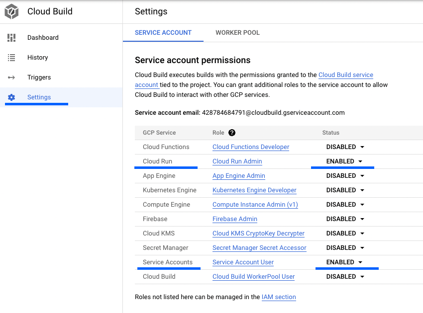
Service Account Berechtigungen für Cloud Run und Service Accounts

Zusammenfassung

Mit Hilfe von Terraform ist es möglich ein vollständig in Code definierten, kontinuierlich veröffentlichten Google Cloud Run Service zu erstellen. Dazu werden GCP Services verwendet, eine Flask Webapp in einem Container zu verpacken und diesen auf Cloud Run zu veröffentlichen.

Für Fragen erstellt gerne ein Issue oder ihr findet mich auf LinkedIn.

Der Quellcode ist in GitHub verfügbar: https://github.com/fingineering/GCPCloudRunDemo

Control the visibility of the PowerBI visuals based on condition

October 6, 2022/in Business Analytics, Business Intelligence, Data Science Hack, Excel / Power BI, Main Category/by Seleha Shaikh

In PowerBI, there is no direct or functional mechanism to adjust the visibility (Show/Hide) of visualizations based on filter choices. There is, however, a workaround that enables us to show/hide visuals based on filter condition.

The fundamental concept behind this technique is to apply a mask to a visual and change its opacity based on a condition or filter selection.

Use Case:

I have detail table of orders. These orders are divided into Consumer, Home Office, and Corporation categories. I use segment as a filter. One of the requirements is to present a table of detail if the overall profit for the selected segment is less than $100,000. To do this, this task will be divided into two major parts. First, we will display the table if the filter is selected. Next, we will add a condition to the table.

Step 1: Show table only filter is selected

Place filter (Slicer) and visual on the Report Pane.

Create a measure that will determine if the filter is selected or not.

Filter_Selected = IF(ISFILTERED(Orders[Segment]),1,0)

Add this measure to the filter pane of the table visualization and select the show item when the value is 1 option. This will ensure that when no options are selected, only the header is displayed.

Set the mask down on the table. Make sure you only mask the table header with a border color that matches your background, or remove it entirely.

Create a measure to change the mask’s transparency. If two zeros are appended to the end of any HAX code, this represents complete transparency.

mask_transparency =IF([Filter_Selected],”#FFFFFF00″,”#FFFFFF”)

Keep this measure on the Fill of the mask and add conditional formatting to it.

If the mask transparency(measure) field is grayed out during the previous steps, you may need to modify the data type of mask transparency to text.

Step 2 : Add a condition to the solution

Create a new measure to determine if our condition is met.

condition_check = IF(CALCULATE(SUM(Orders[Profit]),filter(all(Orders), Orders[Segment] = SELECTEDVALUE(Orders[Segment]))) < 100000,1,0)

Now add this new measure to a table visual’s filter pane and pick the show item when the value is 1 option. This ensures that only if the condition meets the table will appear.

You can now display or hide visuals based on slicer selection and condition. If you know a better way to do this, please comment and let me know. For this article, I referred to this page.

5 Apache Spark Best Practices

July 4, 2022/in Big Data, Data Science Hack, Tool Introduction, Tools/by Sai Priya

Already familiar with the term big data, right? Despite the fact that we would all discuss Big Data, it takes a very long time before you confront it in your career. Apache Spark is a Big Data tool that aims to handle large datasets in a parallel and distributed manner. Apache Spark began as a research project at UC Berkeley’s AMPLab, a student, researcher, and faculty collaboration centered on data-intensive application domains, in 2009.

Introduction

Spark’s aim is to create a new framework that was optimized for quick iterative processing, such as machine learning and interactive data analysis while retaining Hadoop MapReduce’s scalability and fault-tolerant. Spark outperforms Hadoop in many ways, reaching performance levels that are nearly 100 times higher in some cases. Spark has a number of components for various types of processing, all of which are based on Spark Core. Today we will be going to discuss in brief the Apache Spark and 5 of its best practices to look forward to-

What is Apache Spark?

Apache Spark is an open-source distributed system for big data workforces. For fast analytic queries against another size of data, it uses in-memory caching and optimised query execution. It is a parallel processing framework for grouped computers to operate large-scale data analytics applications. This could handle packet and real-time data processing and predictive analysis workloads.

It claims to support code reuse all over multiple workloads—batch processing, interactive queries, real-time analytics, machine learning, and graph processing—and offers development APIs in Java, Scala, Python, and R. With 365,000 meetup members in 2017, Apache Spark is becoming one of the most renowned big data distributed processing frameworks. Explore for Apache Spark Tutorial for more information.

5 best practices of Apache Spark

1. Begin with a small sample of the data.

Because we want to make big data work, we need to start with a small sample of data to see if we’re on the right track. In my project, I sampled 10% of the data and verified that the pipelines were working properly. This allowed me to use the SQL section of the Spark UI to watch the numbers grow throughout the flow while not having to wait too long for it to complete.

In my experience, if you attain your preferred runtime with a small sample, scaling up is usually simple.

2. Spark troubleshooting

For transformations, Spark seems to have a lazy loading behaviour. That is, it will not initiate the transformation computation; instead, it will keep records of the transformation requested. This makes it difficult to determine where in our code there are bugs or areas that need to be optimised. Splitting the code into sections with df.cache() and then using df.count() to force Spark to calculate the df at every section was one practise that we found useful.

Spark actions seem to be keen in that they cause the underlying action to perform a computation. So, if you’ve had a Spark action which you only call when it’s required, pay attention. A Spark action, for instance, is count() on a dataset. You can now inspect the computation of each section using the spark UI and identify any issues. It’s important to note that if you don’t use the sampling we mentioned in (1), you’ll probably end up with a very long runtime that’s difficult to debug.

Check out Apache Spark Training & Certification Course to get yourself certified in Apache Spark with industry-level skills.

3. Finding and resolving Skewness is a difficult task.

Having to look at the stage specifics in the spark UI and looking for just a major difference between both the max and median can help you find the Skewness:

Let’s begin with a definition of Skewness. As previously stated, our data is divided into partitions, and the size of each partition will most likely change as the progress of transformation. This can result in a large difference in size between partitions, indicating that our data is skew. This implies that a few of the tasks were markedly slower than the rest.

Why is this even a bad thing? Because it may cause other stages to stand in line for these few tasks, leaving cores idle. If you understand where all the Skewness has been coming from, you can fix it right away by changing the partitioning.

4. Appropriately cache

Spark allows you to cache datasets in memory. There are a variety of options to choose from:

Since the same operation has been computed several times in the pipeline flow, cache it.
To allow the required cache setting, use the persist API to enable caching (persist to disc or not; serialized or not).
Be cognizant of lazy loading and, if necessary, prime cache up front. Some APIs are eager, while others aren’t.
To see information about the datasets you’ve cached, go to the Storage tab in the Spark UI.
It’s a good idea to unpersist your cached datasets after you’ve finished using them to free up resources, especially if other people are using the cluster.

5. Spark has issues with iterative code.

It was particularly difficult. Spark uses lazy evaluation so that when the code is run, it only creates a computational graph, a DAG. Once you have an iterative process, however, this method can be very problematic so because DAG finally opens the prior iteration and then becomes extremely large, we mean extremely large. This may be too large for the driver to remember. Because the application is stuck, this makes it appear in the spark UI as if no jobs are running (which is correct) for an extended period of time — until the driver crashes.

This seems to be presently an obvious issue with Spark, and the workaround that worked for me was to use df.checkpoint() / df.reset() / df.reset() / df.reset() / df.reset() / df. every 5–6 iterations, call localCheckpoint() (find your number by experimenting a bit). This works because, unlike cache(), checkpoint() breaks the lineage and the DAG, saves the results and starts from a new checkpoint. The disadvantage is that you don’t have the entire DAG to recreate the df if something goes wrong.

Conclusion

Spark is now one of the most popular projects inside the Hadoop ecosystem, with many companies using it in conjunction with Hadoop to process large amounts of data. In June 2013, Spark was acknowledged into the Apache Software Foundation’s (ASF) entrepreneurial context, and in February 2014, it was designated as an Apache Top-Level Project. Spark could indeed run by itself, on Apache Mesos, or on Apache Hadoop, which is the most common. Spark is used by large enterprises working with big data applications because of its speed and ability to connect multiple types of databases and run various types of analytics applications.

Learning how to make Spark work its magic takes time, but these 5 practices will help you move your project forward and sprinkle some spark charm on your code.

process.science presents a new release

December 6, 2021/in Business Analytics, Business Intelligence, Main Category, Process Mining, Sponsoring Partner Posts, Tools/by Editorial Staff

Advertisement

Process Mining Tool provider process.science presents a new release

process.science, specialist in the development of process mining plugins for BI systems, presents its upgraded version of their product ps4pbi. Process.science has added the following improvements to their plug-in for Microsoft Power BI. Identcal upgrades will soon also be released for ps4qlk, the corresponding plug-in for Qlik Sense:

3x faster performance: By improvement of the graph library the graph built got approx. 300% more performant. This is particularly noticeable in complex processes
Navigator window: For a better overview in complex graphs, an overview window has been added, in which the entire graph and the respective position of the viewed area within the overall process is displayed
Activities legend: This allows activities to be assigned to specific categories and highlighted in different colors, for example in which source system an activity was carried out
Activity drill-through: This makes it possible to take filters that have been set for selected activities into other dashboards
Value Color Scale: Activity values can be color-coded and assigned to freely selectable groupings, which makes the overview easier at first sight

process.science Process Mining on Power BI

Process mining is a business data analysis technique. The software used for this extracts the data that is already available in the source systems and visualizes them in a process graph. The aim is to ensure continuous monitoring in real time in order to identify optimization measures for processes, to simulate them and to continuously evaluate them after implementation.

The process mining tools from process.science are integrated directly into Microsoft Power BI and Qlik Sense. A corresponding plug-in for Tableau is already in development. So it is not a complicated isolated solution requires a new set up in addition to existing systems. With process.science the existing know-how on the BI system already implemented and the existing infrastructure framework can be adapted.

The integration of process.science in the BI systems has no influence on day-to-day business and bears absolutely no risk of system failures, as process.science does not intervene in the the source system or any other program but extends the respective business intelligence tool by the process perspective including various functionalities.

Contact person for inquiries:

process.science GmbH & Co. KG
Gordon Arnemann
Tel .: + 49 (231) 5869 2868
Email: ga@process.science
https://de.process.science/

Process Mining mit Fluxicon Disco – Artikelserie

August 30, 2021/in Business Analytics, Business Intelligence, Main Category, Process Mining, Tool Introduction, Tools/by Benjamin Aunkofer

Dieser Artikel der Artikelserie Process Mining Tools beschäftigt sich mit dem Anbieter Fluxicon. Das im Jahr 2010 gegründete Unternehmen, bis heute geführt von den zwei Gründern Dr. Anne Rozinat und Dr. Christian W. Günther, die beide bei Prof. Wil van der Aalst in Eindhoven promovierten, sowie einem weiteren Mitarbeiter, ist eines der ersten Tool-Anbieter für Process Mining. Das Tool Disco ist das Kernprodukt des Fluxicon-Teams und bietet pures Process Mining.

Die beiden Gründer haben übrigens eine ganze Reihe an Artikeln zu Process Mining (ohne Sponsoring / ohne Entgelt) veröffentlicht.

Lösungspakete:	Standard-Lizenz
Zielgruppe:	Lauf Fluxicon für Unternehmen aller Größen.
Datenquellen:	Keine Standard-Konnektoren. Benötigt fertiges Event Log.
Datenvolumen:	Unlimitierte Datenmengen, Beschränkung nur durch Hardware.
Architektur:	On-Premise / Desktop-Anwendung

Diese Software für Process Mining ist für jeden, der in Process Mining reinschnuppern möchte, direkt als Download verfügbar. Die Demo-Lizenz reicht aus, um eigene Event-Logs auszuprobieren oder das mitgelieferte Event-Log (Sandbox) zu benutzen. Es gibt ferner mehrere Evaluierungslizenz-Modelle sowie akademische Lizenzen via Kooperationen mit Hochschulen.

Fluxicon Disco erfreut sich einer breiten Nutzerbasis, die seit 2012 über das jährliche ‘Process Mining Camp’ (https://fluxicon.com/camp/index und http://processminingcamp.com ) und seit 2020 auch über das monatliche ‘Process Mining Café’ (https://fluxicon.com/cafe/) vorangetrieben wird.

Bedienbarkeit und Anpassungsfähigkeit der Analysen

Fluxicon Disco bietet den Vorteil des schnellen Einstiegs in datengetriebene Prozessanalysen und ist überaus nutzerfreundlich für den Analysten. Die Oberflächen sind leicht zu bedienen und die Bedeutung schnell zu erfassen oder zumindest zu erahnen. Die Filter-Möglichkeiten sind überraschend umfangreich und äußerst intuitiv bedien- und kombinierbar.

Fluxicon Disco Process Mining – Das Haupt-Dashboard zeigt den Process Flow aus der Rekonstruktion auf Basis des Event Logs. Hier wird die Frequenz-Ansicht gezeigt, die Häufigkeiten von Cases und Events darstellt.

Disco lässt den Analysten auf Process Mining im Kern fokussieren, es können keine Analyse-Diagramme strukturell hinzugefügt, geändert oder gelöscht werden, es bleibt ein statischer Report ohne weitere BI-Funktionalitäten.

Die Visualisierung des Prozess-Graphen im Bereich “Map” ist übersichtlich, stets gut lesbar und leicht in der Abdeckung zu steuern. Die Hauptmetrik kann zwischen der Frequenz- zur Zeit-Orientierung hin und her geschaltet werden. Neben der Hauptmetrik kann auch eine zweite Metrik (Secondary Metric) zur Ansicht hinzugefügt werden, was sehr sinnvoll ist, wenn z. B. neben der durchschnittlichen Zeit zwischen Prozessaktivitäten auch die Häufigkeit dieser Prozessfolgen in Relation gesetzt werden soll.

Die Ansicht “Statistics” zeigt die wesentlichen Einblicke nach allen Dimensionen aus statistischer Sicht: Welche Prozessaktivitäten, Ressourcen oder sonstigen Features treten gehäuft auf? Diese Fragen werden hier leicht beantwortet, ohne dass der Analyst selbst statistische Berechnungen anstellen muss – jedoch auch ohne es zu dürfen, würde er wollen.

Die weitere Ansicht “Cases” erlaubt einen Einblick in die Prozess-Varianten und alle Einzelfälle innerhalb einer Variante. Diese Ansicht ist wichtig für Prozessoptimierer, die Optimierungspotenziale vor allem in häufigen, sich oft wiederholenden Prozessverläufen suchen möchten. Für Compliance-Analysten sind hingegen eher die oft vielen verschiedenen Einzelfälle spezieller Prozessverläufe der Fokus.

Für Einsteiger in Process Mining als Methodik und Disco als Tool empfiehlt sich übrigens das Process Mining Online Book: https://processminingbook.com

Integrationsfähigkeit

Fluxicon Disco ist eine Desktop-Anwendung, die nicht als Cloud- oder Server-Version verfügbar ist. Es ist möglich, die Software auf einem Windows Application Server on Premise zu installieren und somit als virtuelle Umgebung via Microsoft Virtual Desktop oder via Citrix als virtuelle Anwendung für mehrere Anwender zugleich verfügbar zu machen. Allerdings ist dies keine hochgradige Integration in eine Enterprise-IT-Infrastruktur.

Auch wird von Disco vorausgesetzt, dass Event Logs als einzelne Tabellen bereits vorliegen müssen. Dieses Tool ist also rein für die Analyse vorgesehen und bietet keine Standardschnittstellen mit vorgefertigten Skripten zur automatischen Herstellung von Event Logs beispielsweise aus Salesforce CRM oder SAP ERP.

Grundsätzlich sollte Process Mining methodisch stets als Doppel-Disziplin betrachtet werden: Der erste Teil des Process Minings fällt in die Kategorie Data Engineering und umfasst die Betrachtung der IT-Systeme (ERP, CRM, SRM, PLM, DMS, ITS,….), die für einen bestimmten Prozess relevant sind, und die in diesen System hinterlegten Datentabellen als Datenquellen. Die in diesen enthaltenen Datenspuren über Prozessaktivitäten müssen dann in ein Prozessprotokoll überführt und in ein Format transformiert werden, das der Inputvoraussetzung als Event Log für das jeweilige Process Mining Tool gerecht wird. Minimalanforderung ist hierbei zumindest eine Vorgangsnummer (Case ID), ein Zeitstempel (Event Time) einer Aktivität und einer Beschreibung dieser Aktivität (Event).

Das Event Log kann dann in ein oder mehrere Process Mining Tools geladen werden und die eigentliche Prozessanalyse kann beginnen. Genau dieser Schritt der Kategorie Data Analytics kann in Fluxicon Disco erfolgen.

Zum Einspeisen eines Event Logs kann der klassische CSV-Import verwendet werden oder neuerdings auch die REST-basierte Airlift-Schnittstelle, so dass Event Logs direkt von Servern On-Premise oder aus der Cloud abgerufen werden können.

Prinzip des direkten Zugriffs auf Event Logs von Servern via Airlift.

Import von Event Logs als CSV (“Open file”) oder von Servern auch aus der Cloud.

Sind diese Limitierungen durch die Software für ein Unternehmen, bzw. für dessen Vorhaben, vertretbar und bestehen interne oder externe Ressourcen zum Data Engineering von Event Logs, begeistert die Einfachheit von Process Mining mit Fluxicon Disco, die den schnellsten Start in diese Analyse verspricht, sofern die Daten als Event Log vorbereitet vorliegen.

Skalierbarkeit

Die Skalierbarkeit im Sinne hochskalierender Datenmengen (Big Data Readiness) sowie auch im Sinne eines Ausrollens dieser Analyse-Software auf einer Konzern-Ebene ist nahezu nicht gegeben, da hierzu Benutzer-Berechtigungsmodelle fehlen. Ferner darf hierbei nicht unberücksichtigt bleiben, dass Disco, wie zuvor erläutert, ein reines Analyse-/Visualisierungstool ist und keine Event Logs generieren kann (der Teil der Arbeit, der viele Hardware Ressourcen benötigt).

Für die reine Analyse läuft Disco jedoch auch mit vielen Daten sehr zügig und ist rein auf Ebene der Hardware-Ressourcen limitiert. Vertikales Upscaling ist auf dieser Ebene möglich, dazu empfiehlt sich diese Leselektüre zum System-Benchmark.

Zukunftsfähigkeit

Fluxicon Disco ist eines der Process Mining Tools der ersten Stunde und wird auch heute noch stetig vom Fluxicon Team mit kleinen Updates versorgt, die Weiterentwicklung ist erkennbar, beschränkt sich jedoch auf Process Mining im Kern.

Preisgestaltung

Die Preisgestaltung wird, wie auch bei den meisten anderen Anbietern für Process Mining Tools, nicht transparent kommuniziert. Aus eigener Einsatzerfahrung als Berater können mit Preisen um 1.000 EUR pro Benutzer pro Monat gerechnet werden, für Endbenutzer in Anwenderunternehmen darf von anderen Tarifen ausgegangen werden.

Studierende von mehr als 700 Universitäten weltweit (siehe https://fluxicon.com/academic/) können Fluxicon Disco kostenlos nutzen und das sehr unkompliziert. Sie bekommen bereits automatisch akademische Lizenzen, sobald sie sich mit ihrer Uni-Email-Adresse in dem Tool registrieren. Forscher und Studierende, deren Uni noch kein Partner ist, können sehr leicht auch individuelle akademische Lizenzen anfragen.

Fazit

Fluxicon Disco ist ein Process Mining Tool der ersten Stunde und das bis heute. Das Tool beschränkt sich auf das Wesentliche, bietet keine Big Data Plattform mit Multi-User-Management oder anderen Möglichkeiten integrierter Data Governance, auch sind keine Standard-Schnittstellen zu anderen IT-Systemen vorhanden. Auch handelt es sich hierbei nicht um ein Tool, das mit anderen BI-Tools interagieren oder gar selbst zu einem werden möchte, es sind keine eigenen Report-Strukturen erstellbar. Fluxicon Disco ist dafür der denkbar schnellste Einstieg mit minimaler Rüstzeit in Process Mining für kleine bis mittelständische Unternehmen, für die Hochschullehre und nicht zuletzt auch für Unternehmensberatungen oder Wirtschaftsprüfungen, die ihren Kunden auf schlanke Art und Weise Ist-Prozessanalysen ergebnisorientiert anbieten möchten.

Dass Disco seitens Fluxicon nur für kleine und mittelgroße Unternehmen bestimmt ist, ist nicht ganz zutreffend. Die meisten Kunden sind grosse Unternehmen (Banken, Versicherungen, Telekommunikationsanabieter, Ministerien, Pharma-Konzerne und andere), denn diese haben komplexe Prozesse und somit den größten Optimierungsbedarf. Um Process Mining kommen die Unternehmen nicht herum und so sind oft auch mehrere Tools verschiedener Anbieter im Einsatz, die sich gegenseitig um ihre Stärken ergänzen, für Fluxicon Disco ist dies die flexible Nutzung, nicht jedoch das unternehmensweite Monitoring. Der flexible und schlanke Einsatz von Disco in vielen Unternehmen zeigt sich auch mit Blick auf die Sprecher und Teilnehmer der jährlichen Nutzerkonferenz, dem Process Mining Camp.

Sponsored Post

So why using IaC for Cloud Data Infrastructures?

Version Control for your Cloud Infrastructure

Scalability Tailored for Data Needs

Cost-Efficiency in Resource Allocation

Streamlined Collaboration Among Teams

Enhanced Security and Compliance

Reliable Environment for Data Operations

Documentation and Disaster Recovery Made Easy

Most common IaC solutions

Terraform

Pulumi

Cloud Provider specific IaC Solutions

IaC Tools for Server Configuration

Other types of IaC Solutions

Conclusion

Lambda – Architecture

Kappa – Architecture

Use cases – When to use which architecture?

Requirements that clearly speak for Lambda

Requirements that clearly speak in favor of Kappa:

tl;dr

Voraussetzungen

APIs die in Google Cloud aktiviert werden müssen

Infrastruktur

Die Beispiel Flask Anwendung

Docker Container erstellen, ausführen und deployen

Den ersten Container manuell deployen

Cloud Run Service aufsetzen

Cloud Build Trigger erstellen

Zusammenfassung

Introduction

What is Apache Spark?

5 best practices of Apache Spark

Bedienbarkeit und Anpassungsfähigkeit der Analysen

Integrationsfähigkeit

Skalierbarkeit

Zukunftsfähigkeit

Preisgestaltung

Fazit

Interesting links

Pages

Categories

Archive