A common trap when it comes to sampling from a population that intrinsically includes outliers
I will discuss a common fallacy concerning the conclusions drawn from calculating a sample mean and a sample standard deviation and more importantly how to avoid it.
Suppose you draw a random sample  ,
,  , …
, …  of size
  and compute the ordinary (arithmetic) sample mean
  and a sample standard deviation
  from it. Now if (and only if) the (true) population mean µ (first moment) and population variance (second moment) obtained from the actual underlying PDF are finite, the numbers and make the usual sense otherwise they are misleading as will be shown by an example.
By the way: The common correlation coefficient will also be undefined (or in practice always point to zero) in the presence of infinite population variances. Hopefully I will create an article discussing this related fallacy in the near future where a suitable generalization to Lévy-stable variables will be proposed.
Drawing a random sample from a heavy tailed distribution and discussing certain measures
As an example suppose you have a one dimensional random walker whose step length is distributed by a symmetric standard Cauchy distribution (Lorentz-profile) with heavy tails, i.e. an alpha-stable distribution with alpha being equal to one. The PDF of an individual independent step is given by  , thus neither the first nor the second moment exist whereby the first exists and vanishes at least in the sense of a principal value due to symmetry.
Still let us generate  (pseudo) standard Cauchy random numbers in R* to analyze the behavior of their sample mean and standard deviation as a function of the reduced sample size
  .
.
*The R-code is shown at the end of the article.
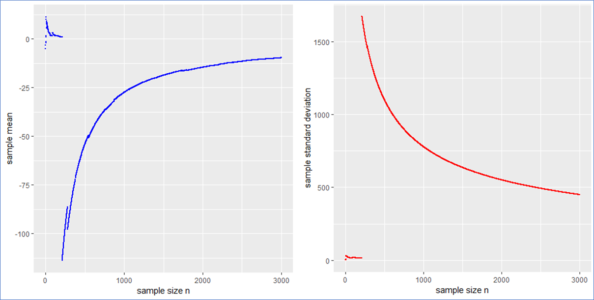
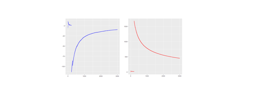
Here are the piecewise sample mean (in blue) and standard deviation (in red) for the mentioned Cauchy sampling. We see that both the sample mean and include jumps and do not converge.
Especially the mean deviates relatively largely from zero even after 3000 observations. The sample has no target due to the population variance being infinite.
If the data is new and no prior distribution is known, computing the sample mean and will be misleading. Astonishingly enough the sample mean itself will have the (formally exact) same distribution as the single step length  . This means that the sample mean is also standard Cauchy distributed implying that with a different Cauchy sample one could have easily observed different sample means far of the presented values in blue.
What sense does it make to present the usual interval  in such a case? What to do?
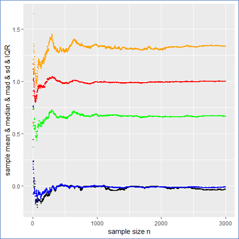
The sample median, median absolute difference (mad) and Inter-Quantile-Range (IQR) are more appropriate to describe such a data set including outliers intrinsically. To make this plausible I present the following plot, whereby the median is shown in black, the mad in green and the IQR in orange.
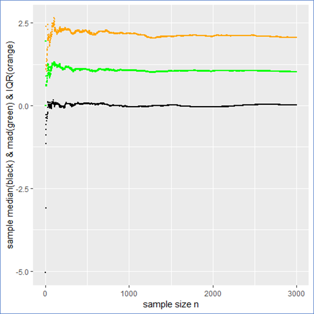
This example shows that the median, mad and IQR converge quickly against their assumed values and contain no major jumps. These quantities do an obviously better job in describing the sample. Even in the presence of outliers they remain robust, whereby the mad converges more quickly than the IQR. Note that a standard Cauchy sample will contain half of its sample in the interval median  mad meaning that the IQR is twice the mad.
Drawing a random sample from a PDF that has finite moments
Just for comparison I also show the above quantities for a standard normal (pseudo) sample labeled with the same color as before as a counter example. In this case not only do both the sample mean and median but also the and mad converge towards their expected values (see plot below). Here all the quantities describe the data set properly and there is no trap since there are no intrinsic outliers. The sample mean itself follows a standard normal, so that the in deed makes sense and one could calculate a standard error  from it to present the usual stochastic confidence intervals for the sample mean.
A careful observation shows that in contrast to the Cauchy case here the sampled mean and converge more quickly than the sample median and the IQR. However still the sampled mad performs about as well as the . Again the mad is twice the IQR.
And here are the graphs of the prementioned quantities for a pseudo normal sample:
The take-home-message:
Just be careful when you observe outliers and calculate sample quantities right away, you might miss something. At best one carefully observes how the relevant quantities change with sample size as demonstrated in this article.
Such curves should become of broader interest in order to improve transparency in the Data Science process and reduce fallacies as well.
Thank you for reading.
P.S.: Feel free to play with the set random seed in the R-code below and observe how other quantities behave with rising sample size. Of course you can also try different PDFs at the beginning of the code. You can employ a Cauchy, Gaussian, uniform, exponential or Holtsmark (pseudo) random sample.
QUIZ: Which one of the recently mentioned random samples contains a trap** and why?
**in the context of this article
R-code used to generate the data and for producing plots:
|
1 2 3 4 5 6 7 8 9 10 11 12 13 14 15 16 17 18 19 20 21 22 23 24 25 26 27 28 29 30 31 32 33 34 35 36 37 38 39 40 41 42 43 44 45 46 47 48 49 50 51 52 53 54 55 56 57 58 59 60 61 62 63 64 65 66 67 68 69 70 71 72 73 74 75 76 77 78 79 80 81 82 83 84 85 86 87 88 89 90 91 92 93 94 95 96 97 |
#R-script for emphasizing convergence and divergence of sample means ####install and load relevant packages #### #uncomment these lines if necessary #install.packages(c('ggplot2',’stabledist’)) #library(ggplot2) #library(stabledist) #####drawing random samples ##### #Setting a random seed for being able to reproduce results set.seed(1234567) N= 2000 #sample size #Choose a PDF from which a sample shall be drawn #To do so (un)comment the respective lines of following code data <- rcauchy(N) # option1(default): standard Cauchy sampling #data <- rnorm(N) #option2: standard Gaussian sampling #data <- rexp(N) # option3: standard exponential sampling #data <- rstable(N,alpha=1.5,beta=0) # option4: standard symmetric Holtsmark sampling #data <- runif(N) #option5: standard uniform sample #####descriptive statistics#### #preparations/declarations SUM = vector() sd =vector() mean = vector() SQ =vector() SQUARES = vector() median = vector() mad =vector() quantiles = data.frame() sem =vector() #piecewise calculaion of descrptive quantities for (k in 1:length(data)){ #mainloop SUM[k] <- sum(data[1:k]) # sum of sample mean[k] <- mean(data[1:k]) # arithmetic mean sd[k] <- sd(data[1:k]) # standard deviation sem[k] <- sd[k]/(sqrt(k)) #standard error of the sample mean (for finite variances) mad[k] <- mad(data[1:k],const=1) # median absolute deviation for (j in 1:5){ qq <- quantile(data[1:k],na.rm = T) quantiles[k,j] <- qq[j] #quantiles of sample } colnames(quantiles) <- c('min','Q1','median','Q3','max') for (i in 1:length(data[1:k])){ SQUARES[i] <- data[i]*data[i] } SQ[k] <- sum(SQUARES[1:k]) #sum of squares of random sample } #end of mainloop #create table containing all relevant data TABLE <- as.data.frame(cbind(quantiles,mean,sd,SQ,SUM,sem)) #####plotting results### x11() print(ggplot(TABLE,aes(1:N,median))+ geom_point(size=.5)+xlab('sample size n')+ylab('sample median')) x11() print(ggplot(TABLE,aes(1:N,mad))+geom_point(size=.5,color ='green')+ xlab('sample size n')+ylab('sample median absolute difference')) x11() print(ggplot(TABLE,aes(1:N,sd))+geom_point(size=.5,color ='red')+ xlab('sample size n')+ylab('sample standard deviation')) x11() print(ggplot(TABLE,aes(1:N,mean))+geom_point(size=.5, color ='blue')+ xlab('sample size n')+ylab('sample mean')) x11() print(ggplot(TABLE,aes(1:N,Q3-Q1))+geom_point(size=.5, color ='blue')+ xlab('sample size n')+ylab('IQR')) #uncomment the following lines of code to see further plots #x11() #print(ggplot(TABLE,aes(1:N,sem))+geom_point(size=.5)+ #xlab('sample size n')+ylab('sample sum of r.v.')) #x11() #print(ggplot(TABLE,aes(1:N,SUM))+geom_point(size=.5)+ #xlab('sample size n')+ylab('sample sum of r.v.')) #x11() #print(ggplot(TABLE,aes(1:N,SQ))+geom_point(size=.5)+ #xlab('sample size n')+ylab('sample sum of squares')) |