After Deep Autoregressive Models, Deep Generative Modelling and Variational Autoencoders we now continue the discussion with Generative Adversarial Networks (GANs).
Introduction
So far, in the series of deep generative modellings (DGMs [Yad22a]), we have covered autoregressive modelling, which estimates the exact log likelihood defined by the model and variational autoencoders, which was variational approximations for lower bound optimization. Both of these modelling techniques were explicitly defining density functions and optimizing the likelihood of the training data. However, in this blog, we are going to discuss generative adversarial networks (GANs), which are likelihood-free models and do not define density functions explicitly. GANs follow a game-theoretic approach and learn to generate from the training distribution through a set up of a two-player game.
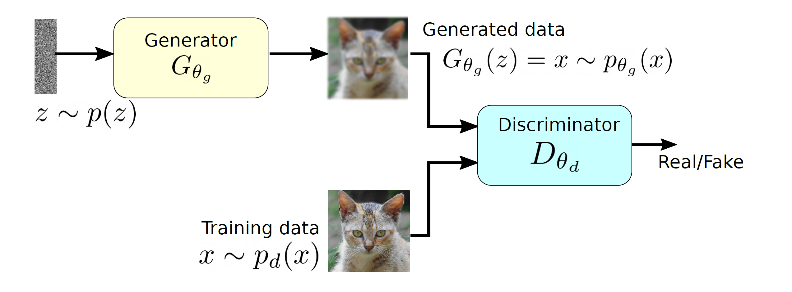
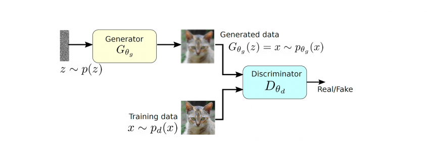
A two player model of GAN along with the generator and discriminators.
GAN tries to learn the distribution of high dimensional training data and generates high-quality synthetic data which has a similar distribution to training data. However, learning the training distribution is a highly complex task therefore GAN utilizes a two-player game approach to overcome the high dimensional complexity problem. GAN has two different neural networks (as shown in Figure ??) the generator and the discriminator. The generator takes a random input  and produces a sample that has a similar distribution as
  . To train this network efficiently, there is the other network that is utilized as the second player and known as the discriminator. The generator network (player one) tries to fool the discriminator by generating real looking images. Moreover, the discriminator network tries to distinguish between real (training data
  ) and fake images effectively. Our main aim is to have an efficiently trained discriminator to be able to distinguish between real and fake images (the generator’s output) and on the other hand, we would like to have a generator, which can easily fool the discriminator by generating real-looking images.
Objective function and training
Objective function
Simultaneous training of these two networks is one of the main challenges in GANs and a minimax loss function is defined for this purpose. To understand this minimax function, firstly, we would like to discuss the concept of two sample testing by Aditya grover [Gro20]. Two sample testing is a method to compute the discrepancy between the training data distribution and the generated data distribution:
(1) ![\begin{equation*} \min_{p_{\theta_g}}\: \max_{D_{\theta_d}\in F} \: \mathbb{E}_{x\sim p_d}[D_{\theta_d}(x)] - \mathbb{E}_{x\sim p_{\theta_g}} [D_{\theta_d}(G_{\theta_g}(x))], \end{equation*}](https://data-science-blog.com/wp-content/ql-cache/quicklatex.com-7980edcee550a3814c1f817f58e1bfb3_l3.png "Rendered by QuickLaTeX.com")
where

and
are the distribution functions of generated and training data respectively. The term

is a set of functions. The \textit{max} part is computing the discrepancies between two distribution using a function

and this part is very similar to the term

(discrepancy measure) from our
first article (Deep Generative Modelling) and KL-divergence is applied to compute this measure in
second article (Deep Autoregressive Models) and
third articles (Variational Autoencoders). However, in GANs, for a given set of functions
, we would like compute the distribution
, which minimizes the overall discrepancy even for a worse function

. The above mentioned objective function does not use any likelihood function and utilizing two different data samples from training and generated data respectively.
By combining Figure ?? and Equation 1, the first term ![\mathbb{E}_{x\sim p_d}[D_{\theta_d}(x)]](https://data-science-blog.com/wp-content/ql-cache/quicklatex.com-1c4b4cb35296fdd7dc76bf9166842c48_l3.png "Rendered by QuickLaTeX.com") corresponds to the discriminator, which has direct access to the training data and the second term
corresponds to the discriminator, which has direct access to the training data and the second term ![\mathbb{E}_{x\sim p_{\theta_g}}[D_{\theta_d}(G_{\theta_g}(x))]](https://data-science-blog.com/wp-content/ql-cache/quicklatex.com-9271a567a190dfafd06b4f7d53f5ffa8_l3.png "Rendered by QuickLaTeX.com") represents the generator part as it relies only on the latent space and produces synthetic data. Therefore, Equation 1 can be rewritten in the form of GAN’s two players as:
represents the generator part as it relies only on the latent space and produces synthetic data. Therefore, Equation 1 can be rewritten in the form of GAN’s two players as:
(2) ![\begin{equation*} \min_{p_{\theta_g}}\: \max_{D_{\theta_d}\in F} \: \mathbb{E}_{x\sim p_d}[D_{\theta_d}(x)] - \mathbb{E}_{z\sim p_z}[D_{\theta_d}(G_{\theta_g}(z))], \end{equation*}](https://data-science-blog.com/wp-content/ql-cache/quicklatex.com-768b9dece98731bd7d56aaa85d15a3d9_l3.png "Rendered by QuickLaTeX.com")
The above equation can be rearranged in the form of log loss:
(3) ![\begin{equation*} \min_{\theta_g}\: \max_{\theta_d} \: (\mathbb{E}_{x\sim p_d} [log \: D_{\theta_d} (x)] + \mathbb{E}_{z\sim p_z}[log(1 - D_{\theta_d}(G_{\theta_g}(z))]), \end{equation*}](https://data-science-blog.com/wp-content/ql-cache/quicklatex.com-bac04040928a64b0805eb863ec4e2864_l3.png "Rendered by QuickLaTeX.com")
In the above equation, the arguments are modified from and  to
to  and
and  respectively as we would like to approximate the network parameters, which are represented by and for the both generator and discriminator respectively. The discriminator wants to maximize the above objective for such that
  , which indicates that the outcome is close to the real data. Furthermore,
  should be close to zero as it is fake data, therefore, the maximization of the above objective function for will ensure that the discriminator is performing efficiently in terms of separating real and fake data. From the generator point of view, we would like to minimize this objective function for such that
  . If the minimization of the objective function happens effectively for then the discriminator will classify a fake data into a real data that means that the generator is producing almost real-looking samples.
Training
The training procedure of GAN can be explained by using the following visualization from Goodfellow et al. [GPAM+14]. In Figure 2(a),  is a random input vector to the generator to produce a synthetic outcome
  (green curve). The generated data distribution is not close to the original data distribution (dotted black curve). Therefore, the discriminator classifies this image as a fake image and forces generator to learn the training data distribution (Figure 2(b) and (c)). Finally, the generator produces the image which could not detected as a fake data by discriminator(Figure 2(d)).
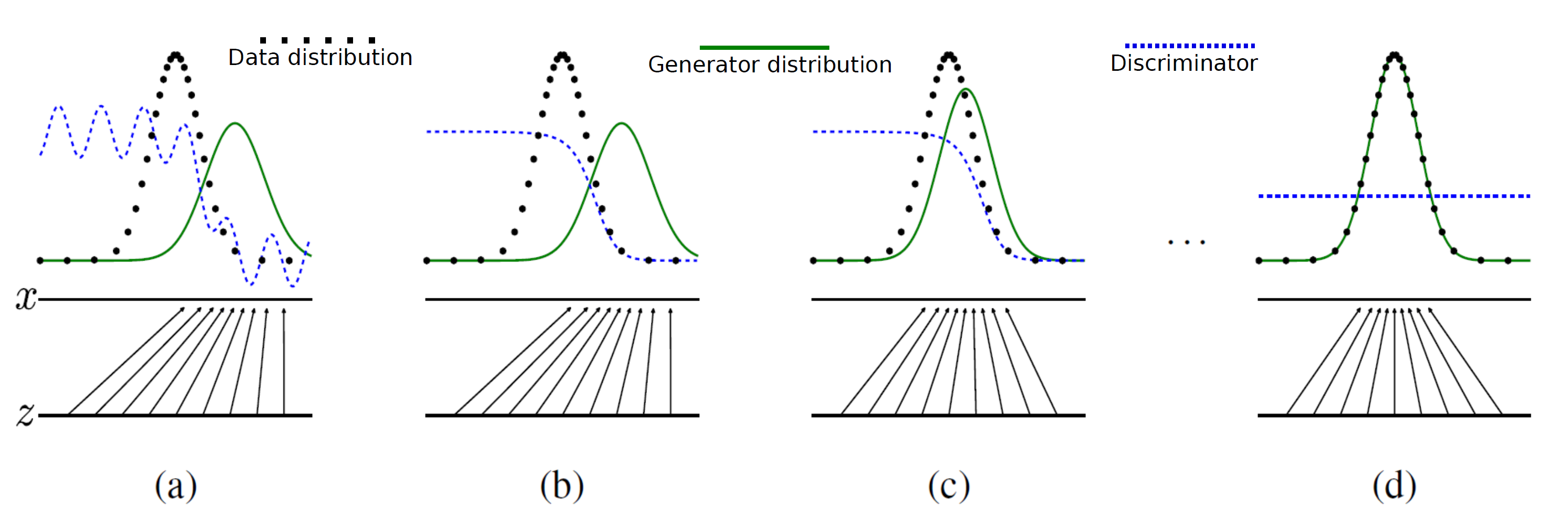
GAN’s training visualization: the dotted black, solid green lines represents pd and pθ
respectively. The discriminator distribution is shown in dotted blue. This image taken from Goodfellow
et al. [GPAM+14].
The optimization of the objective function mentioned in Equation 3 is performed in th following two steps repeatedly:
\begin{enumerate}
\item Firstly, the gradient ascent is utilized to maximize the objective function for for discriminator.
(4) ![\begin{equation*} \max_{\theta_d} \: (\mathbb{E}_{x\sim p_d} [log \: D_{\theta_d}(x)] + \mathbb{E}_{z\sim p_z}[log(1 - D_{\theta_d}(G_{\theta_g}(z))]) \end{equation*}](https://data-science-blog.com/wp-content/ql-cache/quicklatex.com-79cc0abf65c2730d44630b9e9078c251_l3.png "Rendered by QuickLaTeX.com")
\item In the second step, the following function is minimized for the generator using gradient descent.
(5) ![\begin{equation*} \min_{\theta_g} \: ( \mathbb{E}_{z\sim p_z}[log(1 - D_{\theta_d}(G_{\theta_g}(z))]) \end{equation*}](https://data-science-blog.com/wp-content/ql-cache/quicklatex.com-1a5f55cfe2aa160fc40a567edc93237d_l3.png "Rendered by QuickLaTeX.com")
\end{enumerate}
However, in practice the minimization for the generator does now work well because when  then the term
  has the dominant gradient and vice versa.
However, we would like to have the gradient behaviour completely opposite because means the generator is well trained and does not require dominant gradient values. However, in case of  , the generator is not well trained and producing low quality outputs therefore, it requires a dominant gradient for an efficient training. To fix this problem, the gradient ascent method is applied to maximize the modified generator’s objective:
In the second step, the following function is minimized for the generator using gradient descent alternatively.
(6) ![\begin{equation*} \max_{\theta_g} \: \mathbb{E}_{z\sim p_z}[log \: (D_{\theta_d}(G_{\theta_g}(z))] \end{equation*}](https://data-science-blog.com/wp-content/ql-cache/quicklatex.com-20421f265a98722e9835849d78d80269_l3.png "Rendered by QuickLaTeX.com")
therefore, during the training, Equation
4 and
6 will be maximized using the gradient ascent algorithm until the convergence.
Results
The quality of the generated images using GANs depends on several factors. Firstly, the joint training of GANs is not a stable procedure and that could severely decrease the quality of the outcome. Furthermore, the different neural network architecture will modify the quality of images based on the sophistication of the used network. For example, the vanilla GAN [GPAM+14] uses a fully connected deep neural network and generates a quite decent result. Furthermore, DCGAN [RMC15] utilized deep convolutional networks and enhanced the quality of outcome significantly. Furthermore, different types of loss functions are applied to stabilize the training procedure of GAN and to produce high-quality outcomes. As shown in Figure 3, StyleGAN [KLA19] utilized Wasserstein metric [Yad22b] to generate high-resolution face images. As it can be seen from Figure 3, the quality of the generated images are enhancing with time by applying more sophisticated training techniques and network architectures.
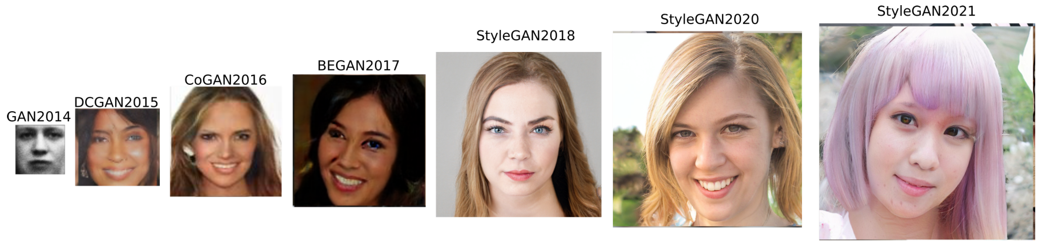
GAN timeline with different variations in terms of network architecture and loss functions.
Summary
This article covered the basics and mathematical concepts of GANs. However, the training of two different networks simultaneously could be complex and unstable. Therefore, researchers are continuously working to create a better and more stable version of GANs, for example, WGAN. Furthermore, different types of network architectures are introduced to improve the quality of outcomes. We will discuss this further in the upcoming blog about these variations.
References
[GPAM+14] Ian Goodfellow, Jean Pouget-Abadie, Mehdi Mirza, Bing Xu, DavidWarde-Farley, Sherjil
Ozair, Aaron Courville, and Yoshua Bengio. Generative adversarial nets. Advances in
neural information processing systems, 27, 2014.
[Gro20] Aditya Grover. Generative adversarial networks.
https://deepgenerativemodels.github.io/notes/gan/, 2020.
[KLA19] Tero Karras, Samuli Laine, and Timo Aila. A style-based generator architecture for
generative adversarial networks. In Proceedings of the IEEE/CVF conference on computer
vision and pattern recognition, pages 4401–4410, 2019.
[RMC15] Alec Radford, Luke Metz, and Soumith Chintala. Unsupervised representation
learning with deep convolutional generative adversarial networks. arXiv preprint
arXiv:1511.06434, 2015.
[Yad22a] Sunil Yadav. Deep generative modelling. https://data-scienceblog.
com/blog/2022/02/19/deep-generative-modelling/, 2022.
[Yad22b] Sunil Yadav. Necessary probability concepts for deep learning: Part 2.
https://medium.com/@sunil7545/kl-divergence-js-divergence-and-wasserstein-metricin-
deep-learning-995560752a53, 2022.

 are initialized to 0, while the policy π(s) is uniformly distributed among all actions. Afterwards, everything is updated through interacting with the stock market environment. By the Bellman Equation,
  is the expectation of the sum of direct reward
  and the future reqard
  at the next state discounted by a factor γ, resulting in the state-action value function:
![[b_t, p_t, h_t, M_t, R_t, C_t, X_t]](https://data-science-blog.com/wp-content/ql-cache/quicklatex.com-0fbdf800e4e901e62bc4396f3815d15f_l3.png "Rendered by QuickLaTeX.com") storing information about
storing information about : Portfolio balance
 : Adjusted close prices
 : Shares owned of each stock
 : Moving Average Convergence Divergence
 : Relative Strength Index
 : Commodity Channel Index
 : Average Directional Index
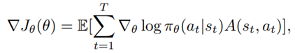
 is the policy network, and
  is the advantage function to reduce the high variance of it:
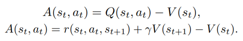
 is the value function of state
  , regardless of actions. DDPG: combines the frameworks of Q-learning and policy gradients and uses neural networks as function approximators; it learns directly from the observations through policy gradient and deterministically map states to actions. The Q-value is updated by:

 https://www.haufe-akademie.de


 dependent variable.