This is the first article of my article series “Instructions on Transformer for people outside NLP field, but with examples of NLP.”
1 Preface
This section is virtually just my essay on language. You can skip this if you want to get down on more technical topic.
As I do not study in natural language processing (NLP) field, I would not be able to provide that deep insight into this fast changing deep leaning field throughout my article series. However at least I do understand language is a difficult and profound field, not only in engineering but also in many other study fields. Some people might be feeling that technologies are eliminating languages, or one’s motivations to understand other cultures. First of all, I would like you to keep it in mind that I am not a geek who is trying to turn this multilingual world into a homogeneous one and rebuild Tower of Babel, with deep learning. I would say I am more keen on social or anthropological sides of language.
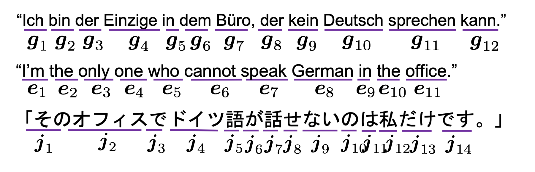
I think you would think more about languages if you have mastered at least one foreign language. As my mother tongue is Japanese, which is totally different from many other Western languages in terms of characters and ambiguity, I understand translating is not what learning a language is all about. Each language has unique characteristics, and I believe they more or less influence one’s personalities. For example, many Western languages make the verb, I mean the conclusion, of sentences clear in the beginning part of the sentences. That is also true of Chinese, I heard. However in Japanese, the conclusion comes at the end, so that is likely to give an impression that Japanese people are being obscure or indecisive. Also, Japanese sentences usually omit their subjects. In German as well, the conclusion of a sentences tend to come at the end, but I am almost 100% sure that no Japanese people would feel German people make things unclear. I think that comes from the structures of German language, which tends to make the number, verb, relations of words crystal clear.
Source: https://twitter.com/nakamurakihiro
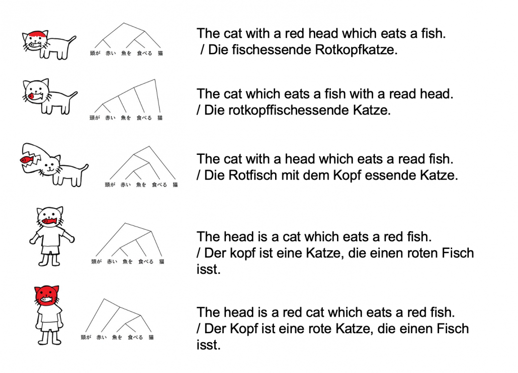
Let’s take an example to see how obscure Japanese is. A Japanese sentence 「頭が赤い魚を食べる猫」can be interpreted in five ways, depending on where you put emphases on.
Common sense tells you that the sentence is likely to mean the first two cases, but I am sure they can mean those five possibilities. There might be similarly obscure sentences in other languages, but I bet few languages can be as obscure as Japanese. Also as you can see from the last two sentences, you can omit subjects in Japanese. This rule is nothing exceptional. Japanese people usually don’t use subjects in normal conversations. And when you read classical Japanese, which Japanese high school students have to do just like Western students learn some of classical Latin, the writings omit subjects much more frequently.
*However interestingly we have rich vocabulary of subjects. The subject “I” can be translated to 「私」、「僕」、「俺」、「自分」、「うち」etc, depending on your personality, who you are talking to, and the time when it is written in.
I believe one can see the world only in the framework of their language, and it seems one’s personality changes depending on the language they use. I am not sure whether the language originally determines how they think, or how they think forms the language. But at least I would like you to keep it in mind that if you translate a conversation, for example a random conversation at a bar in Berlin, into Japanese, that would linguistically sound Japanese, but not anthropologically. Imagine that such kind of random conversation in Berlin or something is like playing a catch, I mean throwing a ball named “your opinion.” On the other hand, normal conversations of Japanese people are in stead more of, I would say, “resonance” of several tuning forks. They do their bests to show that they are listening to each other, by excessively nodding or just repeating “Really?”, but usually it seems hardly any constructive dialogues have been made.
*I sometimes feel you do not even need deep learning to simulate most of such Japanese conversations. Several-line Python codes would be enough.
My point is, this article series is mainly going to cover only a few techniques of NLP in deep learning field: sequence to sequence model (seq2seq model) , and especially Transformer. They are, at least for now, just mathematical models and mappings of a small part of this profound field of language (as far as I can cover in this article series). But still, examples of language would definitely help you understand Transformer model in the long run.
2 Tokens and word embedding
*Throughout my article series, “words” just means the normal words you use in daily life. “Tokens” means more general unit of NLP tasks. For example the word “Transformer” might be denoted as a single token “Transformer,” or maybe as a combination of two tokens “Trans” and “former.”
One challenging part of handling language data is its encodings. If you started learning programming in a language other than English, you would have encountered some troubles of using keyboards with different arrangements or with characters. Some comments on your codes in your native languages are sometimes not readable on some software. You can easily get away with that by using only English, but when it comes to NLP you have to deal with this difficulty seriously. How to encode characters in each language should be a first obstacle of NLP. In this article we are going to rely on a library named BPEmb, which provides word embedding in various languages, and you do not have to care so much about encodings in languages all over the world with this library.
In the first section, you might have noticed that Japanese sentence is not separated with spaces like Western languages. This is also true of Chinese language, and that means we need additional tasks of separating those sentences at least into proper chunks of words. This is not only a matter of engineering, but also of some linguistic fields. Also I think many people are not so conscious of how sentences in their native languages are grammatically separated.
The next point is, unlike other scientific data, such as temperature, velocity, voltage, or air pressure, language itself is not measured as numerical data. Thus in order to process language, including English, you first have to map language to certain numerical data, and after some processes you need to conversely map the output numerical data into language data. This section is going to be mainly about one-hot encoding and word embedding, the ways to convert word/token into numerical data. You might already have heard about this
You might have learnt about word embedding to some extent, but I hope you could get richer insight into this topic through this article.
2.1 One-hot encoding
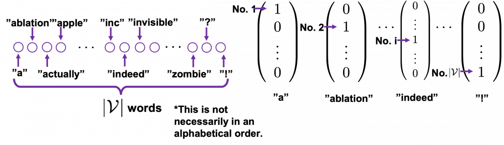
One-hot encoding would be the most straightforward way to encode words/tokens. Assume that you have a dictionary whose size is  , and it includes words from “a”, “ablation”, “actually” to “zombie”, “?”, “!”
In a mathematical manner, in order to choose a word out of those words, all you need is a dimensional vector, one of whose elements is  , and the others are
  . When you want to choose the No. i word, which is “indeed” in the example below, its corresponding one-hot vector is
  , where only the No. i element is . One-hot encoding is also easy to understand, and that’s all. It is easy to imagine that people have already come up with more complicated and better way to encoder words. And one major way to do that is word embedding.
2.2 Word embedding
Source: Francois Chollet, Deep Learning with Python,(2018), Manning
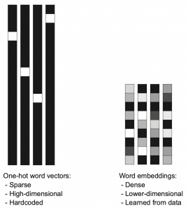
Actually word embedding is related to one-hot encoding, and if you understand how to train a simple neural network, for example densely connected layers, you would understand word embedding easily. The key idea of word embedding is denoting each token with a  dimensional vector, whose dimension is fewer than the vocabulary size . The elements of the resulting word embedding vector are real values, I mean not only 0 or 1. Obviously you can encode much richer variety of tokens with such vectors. The figure at the left side is from “Deep Learning with Python” by François Chollet, and I think this is an almost perfect and simple explanation of the comparison of one-hot encoding and word embedding. But the problem is how to get such convenient vectors. The answer is very simple: you have only to train a network whose inputs are one-hot vector of the vocabulary.
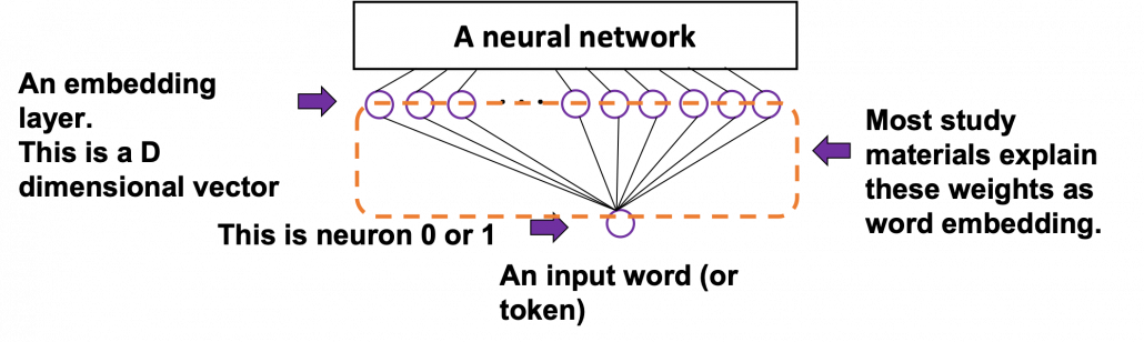
The figure below is a simplified model of word embedding of a certain word. When the word is input into a neural network, only the corresponding element of the one-hot vector is 1, and that virtually means the very first input layer is composed of one neuron whose value is 1. And the only one neuron propagates to the next D dimensional embedding layer. These weights are the very values which most other study materials call “an embedding vector.”
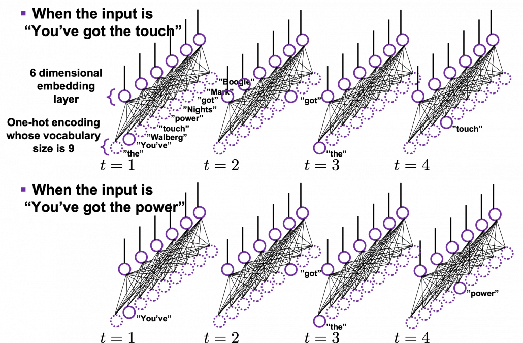
When you input each word into a certain network, for example RNN or Transformer, you map the input one-hot vector into the embedding layer/vector. The examples in the figure are how inputs are made when the input sentences are “You’ve got the touch” and “You’ve got the power.” Assume that you have a dictionary of one-hot encoding, whose vocabulary is {“the”, “You’ve”, “Walberg”, “touch”, “power”, “Nights”, “got”, “Mark”, “Boogie”}, and the dimension of word embeding is 6. In this case  . When the inputs are “You’ve got the touch” or “You’ve got the power” , you put the one-hot vector corresponding to “You’ve”, “got”, “the”, “touch” or “You’ve”, “got”, “the”, “power” sequentially every time step
  .
.
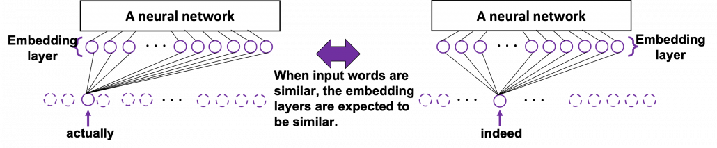
In order to get word embedding of certain vocabulary, you just need to train the network. We know that the words “actually” and “indeed” are used in similar ways in writings. Thus when we propagate those words into the embedding layer, we can expect that those embedding layers are similar. This is how we can mathematically get effective word embedding of certain vocabulary.
More interestingly, if word embedding is properly trained, you can mathematically “calculate” words. For example,  ,
,  .
.
*I have tried to demonstrate this type of calculation on several word embedding, but none of them seem to work well. At least you should keep it in mind that word embedding learns complicated linear relations between words.
I should explain word embedding techniques such as word2vec in detail, but the main focus of this article is not NLP, so the points I have mentioned are enough to understand Transformer model with NLP examples in the upcoming articles.
3 Language model
Language models is one of the most straightforward, but crucial ideas in NLP. This is also a big topic, so this article is going to cover only basic points. Language model is a mathematical model of the probabilities of which words to come next, given a context. For example if you have a sentence “In the lecture, he opened a _.”, a language model predicts what comes at the part “_.” It is obvious that this is contextual. If you are talking about general university students, “_” would be “textbook,” but if you are talking about Japanese universities, especially in liberal art department, “_” would be more likely to be “smartphone. I think most of you use this language model everyday. When you type in something on your computer or smartphone, you would constantly see text predictions, or they might even correct your spelling or grammatical errors. This is language modelling. You can make language models in several ways, such as n-gram and neural language models, but in this article I can explain only general formulations for such models.
*I am not sure which algorithm is used in which services. That must be too fast changing and competitive for me to catch up.
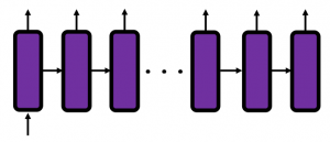
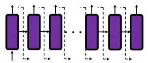
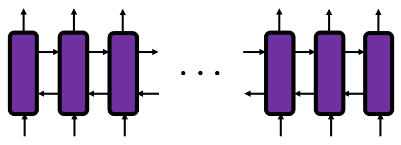
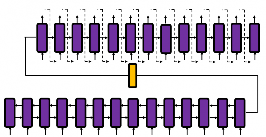
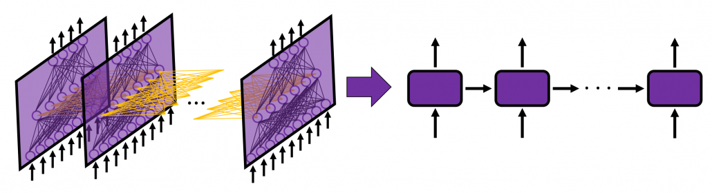
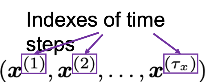
As I mentioned in the first article series on RNN, a sentence is usually processed as sequence data in NLP. One single sentence is denoted as  , a list of vectors. The vectors are usually embedding vectors, and the
  is the index of the order of tokens. For example the sentence “You’ve go the power.” can be expressed as
  , where
  denote “You’ve”, “got”, “the”, “power”, “.” respectively. In this case
  .
.
In practice a sentence  usually includes two tokens
  and
and  at the beginning and the end of the sentence. They mean “Beginning Of Sentence” and “End Of Sentence” respectively. Thus in many cases
  .
.  and
and  are also both vectors, at least in the Tensorflow tutorial.

 is the probability of incidence of the sentence. But it is easy to imagine that it would be very hard to directly calculate how likely the sentence appears out of all possible sentences. I would rather say it is impossible. Thus instead in NLP we calculate the probability
  as a product of the probability of incidence or a certain word, given all the words so far. When you’ve got the words
  so far, the probability of the incidence of
  , given the context is
  .
.  is a probability of the the sentence being
  , and the probability of being
  can be decomposed this way:
 .
.
Just as well 

 .
.
Hence, the general probability of incidence of a sentence is 


 .
.
Let  be and
  be . Plus, let
 ![P(\boldsymbol{x}^{(t+1)}|\boldsymbol{X}_{[0, t]})](https://data-science-blog.com/wp-content/ql-cache/quicklatex.com-9b85b225f0635a7627a99481018f6166_l3.png "Rendered by QuickLaTeX.com") be
be  , then
 ![P(\boldsymbol{X}) = P(\boldsymbol{x}^{(0)})\prod_{t=0}^{\tau}{P(\boldsymbol{x}^{(t+1)}|\boldsymbol{X}_{[0, t]})}](https://data-science-blog.com/wp-content/ql-cache/quicklatex.com-59e2d215f0fea11ec20386dfef220a30_l3.png "Rendered by QuickLaTeX.com") . Language models calculate which words to come sequentially in this way.
. Language models calculate which words to come sequentially in this way.
Here’s a question: how would you evaluate a language model?
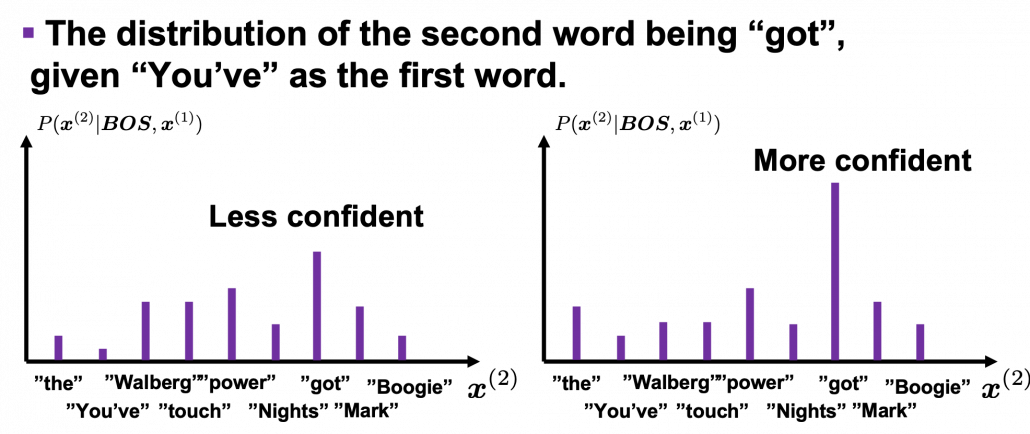
I would say the answer is, when the language model generates words, the more confident the language model is, the better the language model is. Given a context, when the distribution of the next word is concentrated on a certain word, we can say the language model is confident about which word to come next, given the context.
*For some people, it would be more understandable to call this “entropy.”
Let’s take the vocabulary {“the”, “You’ve”, “Walberg”, “touch”, “power”, “Nights”, “got”, “Mark”, “Boogie”} as an example. Assume that 


![P(\boldsymbol{x}^{(0)})\prod_{t=0}^{4}{P(\boldsymbol{x}^{(t+1)}|\boldsymbol{X}_{[0, t]})}](https://data-science-blog.com/wp-content/ql-cache/quicklatex.com-4d263b8554a322d3ab8a8841552bc75b_l3.png "Rendered by QuickLaTeX.com") . Given a context , the probability of incidence of
. Given a context , the probability of incidence of  is
is  . In the figure below, the distribution at the left side is less confident because probabilities do not spread widely, on the other hand the one at the right side is more confident that next word is “got” because the distribution concentrates on “got”.
*You have to keep it in mind that the sum of all possible probability  is , that is,

 .
.
While the language model generating the sentence “BOS You’ve got the touch EOS”, it is better if the language model keeps being confident. If it is confident, 


 gets higher. Thus


 gets lower, where usually
  or
or  .
.
This is how to measure how confident language models are, and the indicator of the confidence is called perplexity. Assume that you have a data set for evaluation  , which is composed of
  sentences in total. Each sentence
![(\boldsymbol{x}^{(0)})\prod_{t=0}^{\tau ^{(n)}}{P(\boldsymbol{x}_{n}^{(t+1)}|\boldsymbol{X}_{n, [0, t]})}](https://data-science-blog.com/wp-content/ql-cache/quicklatex.com-ccc74ac2aee4f90a6b035dcfd2632927_l3.png "Rendered by QuickLaTeX.com") has
has  tokens in total excluding
  . And let be the size of the vocabulary of the language model. Then the perplexity of the language model is
  , where
 ![z = \frac{-1}{|\mathcal{V}|}\sum_{n=1}^{|\mathcal{D}|}{\sum_{t=0}^{\tau ^{(n)}}{log_{b}P(\boldsymbol{x}_{n}^{(t+1)}|\boldsymbol{X}_{n, [0, t]})}](https://data-science-blog.com/wp-content/ql-cache/quicklatex.com-c1ccb76fcad455ad635fc1ec8b2f6f81_l3.png "Rendered by QuickLaTeX.com") . The
. The  is usually
  or
or  .
.
For example, assume that  is vocabulary {“the”, “You’ve”, “Walberg”, “touch”, “power”, “Nights”, “got”, “Mark”, “Boogie”}. Also assume that the evaluation data set for perplexity of a language model is
  , where
 . In this case
 . I have already showed you how to calculate the perplexity of the sentence “You’ve got the touch.” above. You just need to do a similar thing on another sentence “You’ve got the power”, and then you can get the perplexity of the language model.
*If the network is not properly trained, it would also be confident of generating wrong outputs. However, such network still would give high perplexity because it is “confident” at any rate. I’m sorry I don’t know how to tackle the problem. Please let me put this aside, and let’s get down on Transformer model soon.
Appendix
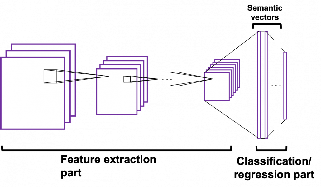
Let’s see how word embedding is implemented with a very simple example in the official Tensorflow tutorial. It is a simple binary classification task on IMDb Dataset. The dataset is composed to comments on movies by movie critics, and you have only to classify if the commentary is positive or negative about the movie. For example when you get you get an input “To be honest, Michael Bay is a terrible as an action film maker. You cannot understand what is going on during combat scenes, and his movies rely too much on advertisements. I got a headache when Mark Walberg used a Chinese cridit card in Texas. However he is very competent when it comes to humorous scenes. He is very talented as a comedy director, and I have to admit I laughed a lot.“, the neural netowork has to judge whether the statement is positive or negative.
This networks just takes an average of input embedding vectors and regress it into a one dimensional value from 0 to 1. The shape of embedding layer is (8185, 16). Weights of neural netowrks are usually implemented as matrices, and you can see that each row of the matrix corresponds to emmbedding vector of each token.
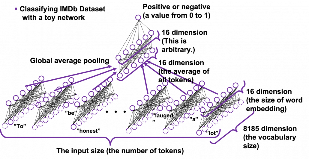
*It is easy to imagine that this technique is problematic. This network virtually taking a mean of input embedding vectors. That could mean if the input sentence includes relatively many tokens with negative meanings, it is inclined to be classified as negative. But for example, if the sentence is “This masterpiece is a dark comedy by Charlie Chaplin which depicted stupidity of the evil tyrant gaining power in the time. It thoroughly mocked Germany in the time as an absurd group of fanatics, but such propaganda could have never been made until ‘Casablanca.'” , this can be classified as negative, because only the part “masterpiece” is positive as a token, and there are much more words with negative meanings themselves.
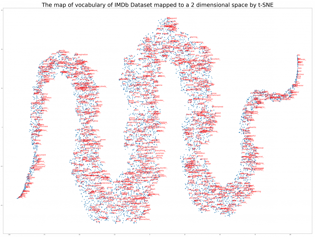
The official Tensorflow tutorial provides visualization of word embedding with Embedding Projector, but I would like you to take more control over the data by yourself. Please just copy and paste the codes below, installing necessary libraries. You would get a map of vocabulary used in the text classification task. It seems you cannot find clear tendency of the clusters of the tokens. You can try other dimension reduction methods to get maps of the vocabulary by for example using Scikit Learn.
1 2 3 4 5 6 7 8 9 10 11 12 13 14 15 16 17 18 19 20 21 22 23 24 25 26 27 28 29 30 31 32 33 34 35 36 37 38 39 40 41 42 43 44 45 46 47 48 49 50 51 52 53 54 55 56 57 58 59 |
import tensorflow as tf from tensorflow import keras from tensorflow.keras import layers import tensorflow_datasets as tfds tfds.disable_progress_bar() (train_data, test_data), info = tfds.load( 'imdb_reviews/subwords8k', split = (tfds.Split.TRAIN, tfds.Split.TEST), with_info=True, as_supervised=True) train_batches = train_data.shuffle(1000).padded_batch(10) test_batches = test_data.shuffle(1000).padded_batch(10) embedding_dim=16 encoder = info.features['text'].encoder model = keras.Sequential([ layers.Embedding(encoder.vocab_size, embedding_dim), layers.GlobalAveragePooling1D(), layers.Dense(16, activation='relu'), layers.Dense(1) ]) print("\n\nThe size of the vocabulary generated from IMDb Dataset is " + str(encoder.vocab_size) + '\n\n') model.summary() model.compile(optimizer='adam', loss=tf.keras.losses.BinaryCrossentropy(from_logits=True), metrics=['accuracy']) history = model.fit( train_batches, epochs=10, validation_data=test_batches, validation_steps=20) word_embedding_vectors = model.layers[0].get_weights()[0] print("\n\nThe shape of the trained weigths of the embedding layer is " + str(word_embedding_vectors.shape) + '\n\n') from sklearn.manifold import TSNE X_reduced = TSNE(n_components = 2, init='pca', random_state=0).fit_transform(word_embedding_vectors) import numpy as np embedding_dict = zip(encoder.subwords, np.arange(len(encoder.subwords))) embedding_dict = dict(embedding_dict) import matplotlib.pyplot as plt plt.figure(figsize=(60, 45)) plt.scatter(X_reduced[:, 0], X_reduced[:, 1]) for i in range(0, len(encoder.subwords), 5): plt.text(X_reduced[i, 0], X_reduced[i, 1], encoder.subwords[i], fontsize=20, color='red') plt.title("The map of vocabulary of IMDb Dataset mapped to a 2 dimensional space by t-SNE", fontsize=60) #plt.savefig('imdb_tsne_map.png') plt.show() |
[References]
[1] “Word embeddings” Tensorflow Core
https://www.tensorflow.org/tutorials/text/word_embeddings
[2]Tsuboi Yuuta, Unno Yuuya, Suzuki Jun, “Machine Learning Professional Series: Natural Language Processing with Deep Learning,” (2017), pp. 43-64, 72-85, 91-94
坪井祐太、海野裕也、鈴木潤 著, 「機械学習プロフェッショナルシリーズ 深層学習による自然言語処理」, (2017), pp. 43-64, 72-85, 191-193
[3]”Stanford CS224N: NLP with Deep Learning | Winter 2019 | Lecture 8 – Translation, Seq2Seq, Attention”, stanfordonline, (2019)
https://www.youtube.com/watch?v=XXtpJxZBa2c
[4] Francois Chollet, Deep Learning with Python,(2018), Manning , pp. 178-185
[5]”2.2. Manifold learning,” scikit-learn
https://scikit-learn.org/stable/modules/manifold.html
* I make study materials on machine learning, sponsored by DATANOMIQ. I do my best to make my content as straightforward but as precise as possible. I include all of my reference sources. If you notice any mistakes in my materials, including grammatical errors, please let me know (email: yasuto.tamura@datanomiq.de). And if you have any advice for making my materials more understandable to learners, I would appreciate hearing it.
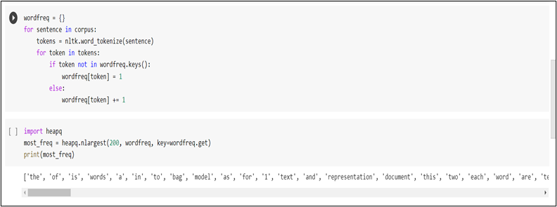
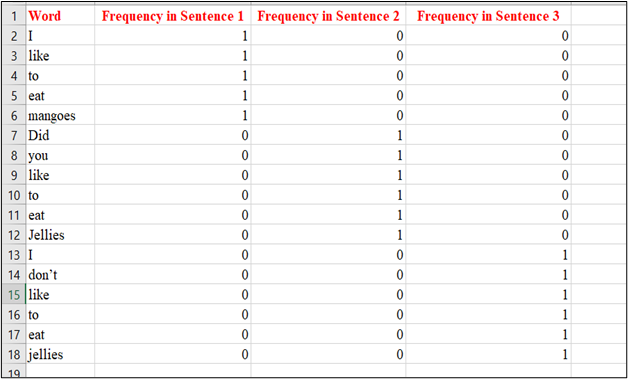
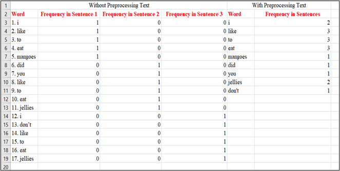

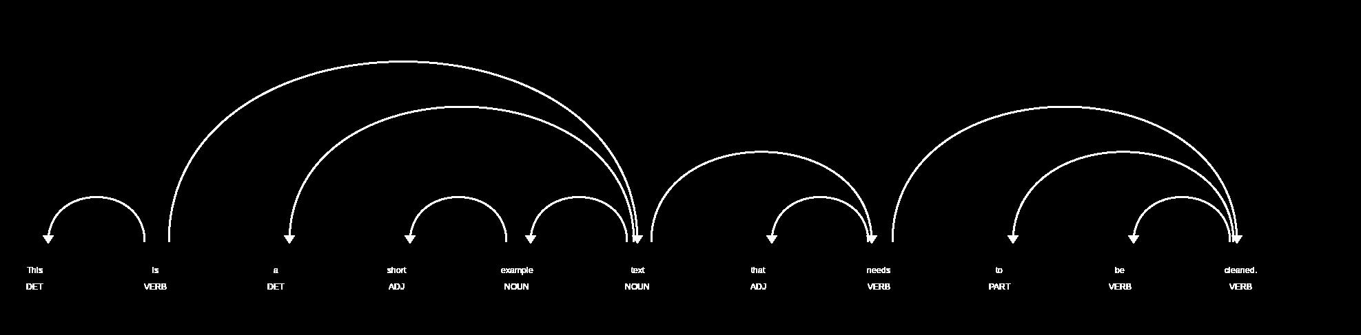
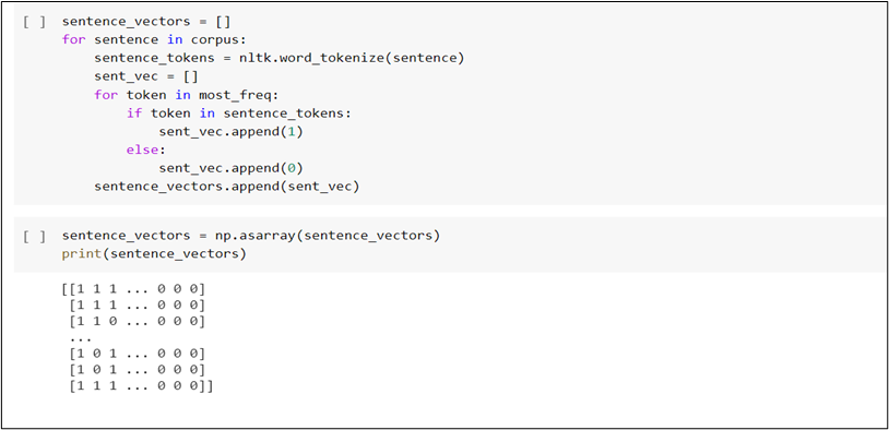
 Step 7: We can observe that the text doesn’t contain any special character or multiple empty spaces, and so our own corpus is ready. The next step is to tokenize each sentence in the corpus and create a dictionary containing each word and their corresponding frequencies.
 , which most people would have seen in compulsory education, is a part of mapping. If you get a value x, you get a value y corresponding to the x.
 . If you have never studied linear algebra , imagine that a vector is a column of Excel data (only one column), a matrix is a sheet of Excel data (with some rows and columns), and a tensor is some sheets of Excel data (each sheet does not necessarily contain only one column.)
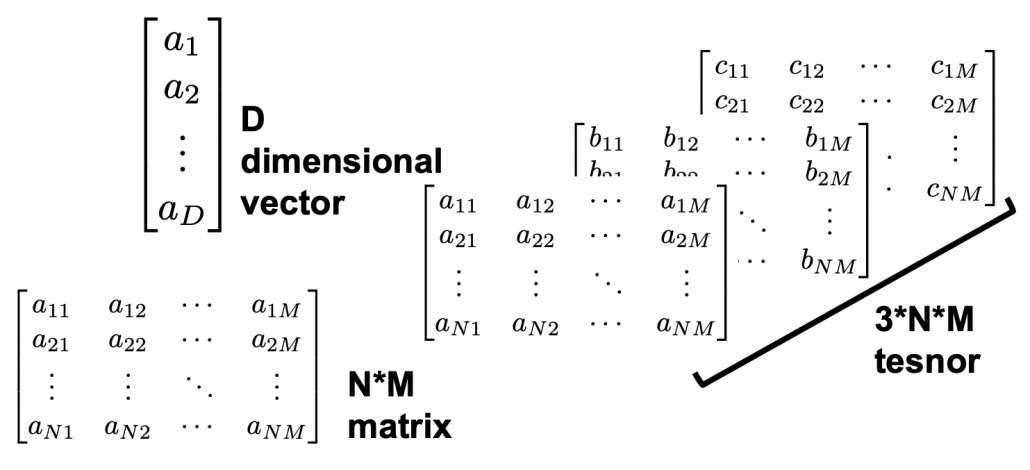

 , and machine translation is nothing but mappings between these sequence data.