How the Internet of Things Technology is Impacting the World

September 29, 2020/in Use Cases/by Walter T. Cassady

Internet of Things, or commonly referred to as IoT, is disrupting industries and arguably making the world a much better place because of it. Some of the main industries are actually listed below.

Manufacturing

The first industry that is seeing a revival from the Internet of Things technology has to be manufacturing. The ways that IoT technology is impacting systems and processes are saving companies and a lot of money and making them more efficient for more profits.

On the factory level, they can predict and presume when a machine needs to go, replaced, or improved upon using IoT technology. On the consumer side of things, they can use the Internet of Things technology to see how customers are using their products, and how they can improve it.

Cars

The automotive industry is also seeing things like connected cars Internet of Things software pop up, and it is changing the industry. The technology lets users get diagnostic information and it lets them be connected to the internet.

Letting users always be connected to the internet is useful in so many areas, and it really would be hard not to find benefit from it.

Public Transportation

Another thing that is related to the general automotive industry is the transportation industry and how the public moves. By using the Internet of Things technology, we can track the diagnostics, fuel, and driver patterns of public transportation.

All of this can increase the effectiveness of public transportation and end up saving the public more money if the drivers are more efficient in the routes that they take across cities.

Housing

The real estate and housing market is the biggest in the world, so naturally, they are going to take advantage of something like the Internet of Things software.

We are starting to see the housing sector take up on smart products in their home, but the Internet of Things is going to eventually make the whole home smart. A refrigerator connected to the internet is most likely coming if you think about it.

While it may seem weird to have everything connected and no appliances are just old school, you can certainly expect this to happen soon. The only problem is, most of the old appliances need to go bad before people have the urge to go out and get a new appliance that is connected to the internet.

Energy and Utilities

The utility market is exploding with the growth of the IoT software because of its many uses. Before, we used to have someone come and read your meter or check for leaks. Now, the connectivity of everything can be monitored from another place, and no one has to show up to your house to read a meter.

It really is a win-win situation for both providers and consumers in the utility and energy sector. It will be very interesting to see how the Internet of Things impacts the world and flips some industries on their side.

DIE Konferenz für Digital Analysts

September 28, 2020/in Data Science News, Events, Recommendations/by events

Optimieren Sie den Einsatz von Daten für Ihr Marketing

Lernen Sie am 16. und 17. November 2020 auf der Marketing Analytics Summit in Berlin alles, was wichtig ist, um datengetriebenes Marketing zu meistern und treffen Sie Kollegen und Experten, die den Unterschied machen.

Sie haben die Wahl zwischen Keynotes, Teilnehmerdiskussionen und -aktionen, Präsentationen und Workshops zu den Themen:

Data Strategy & Governance

Data Driven Culture
Datenarchitektur und -management
Data Literacy
Data Privacy
Datenqualität

2.Technology & Tools

Tracking & Analytics Tools
Neue Technologien & deren Implementierung
Make or Buy Entscheidungen (Tools & Datenhaltung)

KPIs, Dashboard & Visual Analytics

KPI Definition und Steuerung
Graphische Darstellung von Daten/KPIs
Reporting

MarketingAnalytics & Applications

Machine Learning & AI Anwendungen im Marketing
Mulitvariate Analysemethoden
Personalisierung im Marketing
Social Media Analytics
Customer Journey Analysen
Kampagnenauswertung und -optimierung
Marketingattribution

Zwei Tage volles Programm

Vervielfachen Sie Ihr Wissen und Können mit den neuesten Erkenntnissen, aktuellsten Entwicklungen und den relevantesten Beispielen datengestützten Marketings. Lernen Sie eine neue Generation von Marketing-Tools, Techniken und Strategien kennen und vernetzen Sie sich mit Entwicklern und Anwendern!

Kollegen und Experten präsentieren und diskutieren den Einsatz von Digital Analytics, Customer Insights und künstlicher Intelligenz im Marketing. Lernen Sie eine neue Generation von Marketing-Tools, Techniken und Strategien kennen und vernetzen Sie sich mit Entwicklern und Anwendern.

Lassen Sie sich wertvolle Tipps und Tricks von erfahrenen Experten aus namhaften Unternehmen nicht entgehen!

Mit dem Code „DATASCIENCEPAW“ bekommen Sie zusätzliche 15 Prozent Rabatt auf Ihre Buchung.

How the Pandemic is Changing the Data Analytics Outsourcing Industry

September 28, 2020/in Business Analytics, Data Warehousing, Insights, Main Category/by Philip Piletic

While media pundits have largely focused on the impact of COVID-19 as far as human health is concerned, it hasn’t been particularly good for the health of automated systems either. As cybersecurity budgets plummet in the face of dwindling finances, computer criminals have taken the opportunity to increase attacks against high value targets.

In June, an online antique store suffered a data breach that contained over 3 million records, and it’s likely that a number of similar attacks have simply gone unpublished. Fortunately, data scientists are hard at work developing new methods of fighting back against these kinds of breaches. Budget constraints and a lack of personnel as a result of the pandemic continues to be a problem, but automation has helped to assuage the issue to some degree.

AI-Driven Data Storage Systems

Big data experts have long promoted the cloud as an ideal metaphor for the way that data is stored remotely, but as a result few people today consider the physical locations that this information is stored at. All data has to be located on some sort of physical storage device. Even so-called serverless apps have to be distributed from a server unless they’re fully deployed using P2P services.

Since software can never truly replace hardware, researchers are looking at refining the various abstraction layers that exist between servers and the clients who access them. Data warehousing software has enabled computer scientists to construct centralized data storage solutions that look like traditional disk locations. This gives users the ability to securely interact with resources that are encrypted automatically.

Background services based on artificial intelligence monitor virtual data warehouse locations, which gives specialists the freedom to conduct whatever analytics they deem necessary. In some cases, a data warehouse can even anonymize information as it’s stored, which can streamline workflows involved with the analysis process.

While this level of automation has proven useful, it’s still subject to some of the problems that have occurred as a result of the pandemic. Traditional supply chains are in shambles and a large percentage of technical workers are now telecommuting. If there’s a problem with any existing big data plans, then there’s often nobody around to do any work in person.

Living with Shifting Digital Priorities

Many businesses were in the process of outsourcing their data operations even before the pandemic, and the current situation is speeding this up considerably. Initial industry estimates had projected steady growth numbers for the data analytics sector through 2025. While the current figures might not be quite as bullish, it’s likely that sales of outsourcing contracts will remain high.

That being said, firms are also shifting a large percentage of their IT spending dollars into cybersecurity projects. A recent survey found that 37 percent of business leaders said they were already going to cut their IT department budgets. The same study found that 28 percent of businesses are going to move at least some part of their data analytics programs abroad.

Those companies that can’t find an attractive outsourcing contract might start to patch their remote systems over a virtual private network. Unfortunately, this kind of technology has been strained to some degree in recent months. The virtual servers that power VPNs are flooded with requests, which in turn has brought them down in some instances. Neural networks, which utilize deep learning technology to improve themselves as time goes on, have proven more than capable of predicting when these problems are most likely to arise.

That being said, firms that deploy this kind of technology might find that it still costs more to work with automated technology on-premise compared to simply investing in an outsourcing program that works with these kinds of algorithms at an outside location.

Saving Money in the Time of Corona

Experts from Think Big Analytics pointed out how specialist organizations can deal with a much wider array of technologies than a small business ever could. Since these companies specialize in providing support for other organizations, they have a tendency to offer support for a large number of platforms.

These representatives recently opined that they could provide support for NoSQL, Presto, Apache Spark and several other emerging platforms at the same time. Perhaps most importantly, these organizations can work with Hadoop and other traditional data analysis languages.

Staffers working on data mining operations have long relied on languages like Hadoop and R to write scripts that they later use to automate the process of collecting and analyzing data. By working with an organization that already supports a language that companies rely on, they can avoid the need of changing up their existing operations.

This can help to drastically reduce the cost of migration, which is extremely important since many of the firms that need to migrate to a remote system are already suffering from budget problems. Assuming that some issues related to the pandemic continue to plague businesses for some time, it’s likely that these budget constraints will force IT departments to consider a migration even if they would have otherwise relied solely on a traditional colocation arrangement.

IT department staffers were already moving away from many rare platforms even before the COVID-19 pandemic hit, however, so this shouldn’t be as much of a herculean task as it sounds. For instance, the KNIME Analytics Platform has increased in popularity exponentially since it’s release in 2006. The fact that it supports over 1,000 plug-in modules has made it easy for smaller businesses to move toward the platform.

The road ahead isn’t going to be all that pleasant, however. COBOL and other antiquated languages still rule the roost at many governmental big data processing centers. At the same time, some small businesses have never even been able to put a big data plan into play in the first place. As the pandemic continues to wreak havoc on the world’s economy, however, it’s likely that there will be no shortage of organizations continuing to migrate to more secure third-party platforms backed by outsourcing contracts.

How Tech Helps Keep You Safe Throughout the Day

September 27, 2020/in Insights/by James Daniels

Safety is always a primary concern for people no matter what is happening in the world, but there are certain times when it’s pushed firmly to the front of our minds. It’s in these times that we realise just how much we have come to rely on technology to help secure our safety.

From the moment we wake up, to the moment we go to bed, there’s always some sort of technology helping to keep us safe – protecting our health, loved ones and personal details.

Here are just some of the main ways in which tech helps keep you secure throughout the day.

At Home

We literally have everything at the push of a button these days. Whether you want to see who’s at your front door, or check for the latest safety announcements, you’ve got the power to do it with your phone.

Knowledge is power as they say, and having access to limitless information can help keep you safe. When problems do occur, your ability to communicate with people who can help you is also far superior to what has ever been in the past.

Through easy access to information, and clear communication channels, technology has made us more secure at home.

In Hospitals

If you do get sick, then technology is always there to help you get back on your feet. Everyday across the world, research is taking place that improves our medical procedures and makes our medicines more effective.

With novel medicines delivered by innovative drug discovery platform, each day brings us closer to curing previously uncurable diseases and improving the performances of our healthcare systems. Technology is constantly driving the healthcare system forward, helping to make you safer if you do end up in hospital.

On the Road

While you’re still very safe on the road, driving is one of the riskier activities you do on a daily basis. To help protect you, car manufacturers and regulatory bodies are constantly investing in new technology to help keep us safe.

We take amenities such as seatbelts and airbags for granted these days, but they’re part of a constant stream of technologies designed to keep us safer on the roads.

Today we talk about ideas such as lane assist, and even driverless cars to keep us safe, and technology will continue to drive safety forward.

At Work

Workplace accidents are another risk we face when we leave the house, but again, technology is helping to lower the risk and even prevent these from happening.

This can be anything from ergonomic chairs, to sophisticated personnel management systems, but all industries continue to make strides toward keeping you safer when you’re at work.

Online

It’s not so long ago that this wouldn’t have even featured on the list, but we spend so much of our lives online, and store so much of our information there that we have to make sure we’re using it safely.

As quickly as the internet develops, so too does the technology to help keep us safe online. The technology is there to help you, but you’ve got to be aware of the threat and be up to date with online security.

In-memory Data Grid vs. Distributed Cache: Which is Best?

September 25, 2020/in Tool Introduction/by Edward Huskin

Distributed caching has been a boon for IT professionals in the past due to its ability to make data always available even when offline. However, with the growing popularity of the Internet of Things (IoT) and the increasing amounts of data businesses need to process daily, distributed caching is slowly being overshadowed by a newer and more robust technology solution—the in-memory data grid (IMDG).

Distributed caches allow organizations to combine the amount of memory of computers within a network, boosting performance at minimum cost because there’s no need to purchase more disk storage or more high-end computers. Essentially, a data cache is distributed among all networked computers so that applications can use all available memory when needed. Memory is pooled into a single data store or data cache to provide faster access to data. Distributed caches are typically housed in a single physical server kept on site.

The main challenge of distributed caching today is that in-memory data grids can do distributed caching—and much more. What used to be complicated tasks for data analysts and IT professionals has been made simpler and more accessible to the layman. Data analytics, in particular, has become vital for businesses, especially in the areas of marketing and customer service. Nowadays, there are solutions available that present data via graphs and other visualizations to make data mining and analysis less complicated and quicker. The in-memory data grid is one such solution, and is one that’s gradually gaining popularity in the business intelligence (BI) space.

In-memory computing has almost pushed the distributed cache to a realm of obsolescence, so much so, that the remaining organizations that gold onto it as a solution are those that are afraid to embrace digital transformation or those that do not have the resources. However, this doesn’t mean that the distributed cache is less important in the history of computing. In its heyday, distributed caching helped solve a lot of IT infrastructure problems for a number of businesses and industries, and it did all of that at minimal cost.

Distributed Cache for High Availability

The main goal of the distributed cache is to make data always available, which is most useful for companies that require constant access to data, such as mobile applications that store information like user profiles or historical data. Common use cases for distributed caching include payment computations, external web service calls, and dynamic data like number of views or followers. The main draw, however, is how it allows users to access cached data whether the user is online or offline, which, in today’s always-connected world, is a major benefit. Distributed caches take note of frequently accessed data and keep them in process memory so there’s no need to repeatedly access disk storage to get to that data.

Typically, distributed caches offered simplicity through simple “put” and “get” operations through distributed key/value stores. They’re flexible enough, however, to handle more complicated processes through read-through and write-through instances that allow caches to read and write values to and from disk. Depending on the implementation, it can also handle ACID transactions, data replication, and active backups. Ultimately, distributed caching can help handle large, unpredictable amounts of data without sacrificing read consistency.

In-memory Data Grid for High Speed and Much More

The in-memory data grid (IMDG) is not just a storage solution; it’s a powerful computing solution that has the capability to do distributed caching and more. Designed to use RAM and eliminate the need for constant access to disk-based storage, an IMDG is able to process complex data for large-scale implementations at high speeds. Similar to distributed caching, it “distributes” the workload to a multitude of computers within a network, not only combining available RAM but also the computing power of all available computers.

An IMDG runs specialized software on each computer to enable this and to minimize movement of data to and from disk and within the network. Limiting physical disk access eliminates the bottlenecks usually caused by disk-based storage, since using disk in data processing means using an intermediary physical server to move data from one storage system to another. Consistent data synchronicity is also a highlight of the IMDG. This addresses challenges brought about by the complexity of data retrieval and updating, helping to speed up application development. An IMDG also allows both the application and its data to collocate in a single memory space to minimize latency.

Overall, the IMDG is a cost-effective solution because it all but eliminates the complexities and challenges involved in handling disk-based storage. It’s also highly scalable because its architecture is designed to scale horizontally. IMDG implementations can be scaled by simply adding new nodes to an existing cluster of server nodes.

In-memory Computing for Business

Businesses that have adopted in-memory solutions currently enjoy the platform’s relative simplicity and ease of use. Self-service is the ultimate goal of in-memory computing solutions, and this design philosophy is helping typical users transition into “power users” that expect high performance and more sophisticated features and capabilities.

The rise of in-memory computing may be a telltale sign of the distributed cache’s eventual exit, but it still retains its use, especially for organizations that are just looking to address current needs. It might not be an effective solution in the long run, however, as the future leans toward hybrid data and in-memory computing platforms that are more than just data management solutions.

5 Data Privacy Predictions for 2021

September 22, 2020/in Data Security/by Shannon Flynn

2020 has been a significant year for data management. As businesses face new technological challenges amid the COVID-19 pandemic, issues of privacy have spent some time in the spotlight. In response, data privacy could see some substantial changes in 2021.

Few people will emerge from 2020 with an unchanged perception of data security. As these ideas and feelings shift, some trends will accelerate while others get replaced. Businesses will have to adapt to these changes to survive.

Here are five such changes you can expect in 2021.

International Data Privacy Standards Will Increase

Privacy concerns over Chinese-owned app TikTok caused quite a stir in 2020. With the TikTok situation bringing new attention to privacy in international services, you’ll likely see a rise in international regulations. China has already announced new security standards and asked other countries to follow.

2020 has cast doubt over a lot of international relations. More countries will likely issue new standards to ease tension and move past these doubts. This trend started before 2020, as you can see in Europe’s GDPR, but 2021 will further it.

Customers Will Demand Transparency

Governments aren’t the only ones that will expect more of tech companies’ privacy standards. Since things like TikTok have made people more aware of what apps could access, more people will demand privacy. In 2021, companies that are transparent about how they use data will likely be more successful.

According to a PwC poll, 84% of consumers said they would switch services if they don’t trust how a company uses their data. Data privacy isn’t just important to authorities or businesses anymore. The public is growing more concerned about their data, and their choices will reflect it.

Security Will Become More Automated

In response to these growing expectations, businesses will have to do more to secure people’s data. Cybersecurity companies are facing a considerable talent shortage thanks to pandemic-related complications, though. The data security world will turn to automation to fix both of these problems.

With so many businesses changing the way they operate, cybersecurity will have to become more flexible too. Automating some processes through AI will allow companies to achieve that flexibility. Security AI is still relatively new, but as it develops, it could take off in 2021.

Security Data Analytics Will Become the Norm

Big data analytics have already become standard practice in many business applications. In 2021, more companies will start using them to improve their data privacy measures, too. With major companies like Nintendo and Marriott experiencing significant data breaches this year, more will turn to analytics to find any potential shortcomings.

No one wants to be the next data breach news story, especially with more people paying attention to these issues now. Data analytics can highlight operational improvements, showing companies how to better their data security measures. With data privacy in the spotlight in 2021, taking these steps is crucial.

Third-Party Risk Assessments Will Be More Crucial

As people demand better privacy protection, businesses will have to consider their third-party partners. Consumers will be more critical of companies giving third parties access to their data. As a result, companies will have to perform more risk assessments on any third party.

Third-party data breaches affected companies like General Electric and T-Mobile in 2020, exposing thousands of records. Customers will expect businesses to hold their partners to higher standards to avoid these risks.

2021 Could Be a Landmark Year for Data Privacy

Data privacy is more prominent than ever before, mostly due to a few notable scandals. Now that the general public is more aware of these issues, businesses will have to meet higher standards for data privacy. Implementing data security processes may cause some disruption and confusion at first, but it will ultimately lead to a safer digital landscape.

All of these changes could make 2021 a turning point for data security. With higher expectations from consumers and authorities, data management will become more secure.

Data Science in Engineering Process - Product Lifecycle Management

How to develop digital products and solutions for industrial environments?

September 18, 2020/in Data Science, Insights, Main Category, Use Case, Use Cases/by Siemens Advanta Consulting

The Data Science and Engineering Process in PLM.

Huge opportunities for digital products are accompanied by huge risks

Digitalization is about to profoundly change the way we live and work. The increasing availability of data combined with growing storage capacities and computing power make it possible to create data-based products, services, and customer specific solutions to create insight with value for the business. Successful implementation requires systematic procedures for managing and analyzing data, but today such procedures are not covered in the PLM processes.

From our experience in industrial settings, organizations start processing the data that happens to be available. This data often does not fully cover the situation of interest, typically has poor quality, and in turn the results of data analysis are misleading. In industrial environments, the reliability and accuracy of results are crucial. Therefore, an enormous responsibility comes with the development of digital products and solutions. Unless there are systematic procedures in place to guide data management and data analysis in the development lifecycle, many promising digital products will not meet expectations.

Various methodologies exist but no comprehensive framework

Over the last decades, various methodologies focusing on specific aspects of how to deal with data were promoted across industries and academia. Examples are Six Sigma, CRISP-DM, JDM standard, DMM model, and KDD process. These methodologies aim at introducing principles for systematic data management and data analysis. Each methodology makes an important contribution to the overall picture of how to deal with data, but none provides a comprehensive framework covering all the necessary tasks and activities for the development of digital products. We should take these approaches as valuable input and integrate their strengths into a comprehensive Data Science and Engineering framework.

In fact, we believe it is time to establish an independent discipline to address the specific challenges of developing digital products, services and customer specific solutions. We need the same kind of professionalism in dealing with data that has been achieved in the established branches of engineering.

Data Science and Engineering as new discipline

Whereas the implementation of software algorithms is adequately guided by software engineering practices, there is currently no established engineering discipline covering the important tasks that focus on the data and how to develop causal models that capture the real world. We believe the development of industrial grade digital products and services requires an additional process area comprising best practices for data management and data analysis. This process area addresses the specific roles, skills, tasks, methods, tools, and management that are needed to succeed.

*Figure: Data Science and Engineering as new engineering discipline*

More than in other engineering disciplines, the outputs of Data Science and Engineering are created in repetitions of tasks in iterative cycles. The tasks are therefore organized into workflows with distinct objectives that clearly overlap along the phases of the PLM process.

	Feasibility of Objectives
	Understand the business situation, confirm the feasibility of the product idea, clarify the data infrastructure needs, and create transparency on opportunities and risks related to the product idea from the data perspective.
	Domain Understanding
	Establish an understanding of the causal context of the application domain, identify the influencing factors with impact on the outcomes in the operational scenarios where the digital product or service is going to be used.
	Data Management
	Develop the data management strategy, define policies on data lifecycle management, design the specific solution architecture, and validate the technical solution after implementation.
	Data Collection
	Define, implement and execute operational procedures for selecting, pre-processing, and transforming data as basis for further analysis. Ensure data quality by performing measurement system analysis and data integrity checks.
	Modeling
	Select suitable modeling techniques and create a calibrated prediction model, which includes fitting the parameters or training the model and verifying the accuracy and precision of the prediction model.
	Insight Provision
	Incorporate the prediction model into a digital product or solution, provide suitable visualizations to address the information needs, evaluate the accuracy of the prediction results, and establish feedback loops.

Real business value will be generated only if the prediction model at the core of the digital product reliably and accurately reflects the real world, and the results allow to derive not only correct but also helpful conclusions. Now is the time to embrace the unique chances by establishing professionalism in data science and engineering.

Authors

Peter Louis

Peter Louis is working at Siemens Advanta Consulting as Senior Key Expert. He has 25 years’ experience in Project Management, Quality Management, Software Engineering, Statistical Process Control, and various process frameworks (Lean, Agile, CMMI). He is an expert on SPC, KPI systems, data analytics, prediction modelling, and Six Sigma Black Belt.

Ralf Russ

Ralf Russ works as a Principal Key Expert at Siemens Advanta Consulting. He has more than two decades experience rolling out frameworks for development of industrial-grade high quality products, services, and solutions. He is Six Sigma Master Black Belt and passionate about process transparency, optimization, anomaly detection, and prediction modelling using statistics and data analytics.4

Process Mining mit PAFnow – Artikelserie

September 15, 2020/in Business Analytics, Business Intelligence, Process Mining, Tool Introduction, Tools/by Jurek Dörner

Artikelserie zu Process Mining Tools – PAFnow

Der zweite Artikel der Artikelserie Process Mining Tools beschäftigt sich mit dem Anbieter PAFnow. 2014 in Deutschland gegründet kann das Unternehmen PAF, dessen Kürzel für Process Analytics Factory steht, bereits auf eine beachtliche Anzahl an Projekten zurückblicken. Das klare selbst gesteckte Ziel von PAF: Mit dem eigenen Tool namens PAFnow Process Mining für jeden zugänglich machen.

PAFnow basiert auf dem bekannten BI-Tool „Power BI“. Wer sein Wissen zu Power BI noch einmal auffrischen möchte, kann das gerne in diesem Artikel aus der Artikelserie zu BI-Tools machen. Da Power BI selbst als Cloud- und On-Premise-Lösung erhältlich ist, gilt dies indirekt auch für PAFnow. Diese vier Versionen des Process Mining Tools werden von PAFnow angeboten:

	Free	Pro	Premium	Enterprise
Lizenz:	Kostenfrei (Marketplace Power BI)	99€ pro User pro Monat	499€ pro User pro Monat	Nur auf Anfrage
Zielgruppe:	Für kleine Unternehmen und Einzelanwender	Für kleine bis mittlere Unternehmen	Für mittlere und große Unternehmen	Für mittlere und große Unternehmen
Datenquellen:	Beliebig (Power BI Konnektoren), Transformationen in Power BI	Beliebig (Power BI Konnektoren), Transformationen in Power BI	Beliebig (Power BI Konnektoren), Transformationen in Power BI	Beliebig (Power BI Konnektoren), Transformationen auch via MS SSIS
Datenvolumen:	Limitiert auf 30.000 Events, 1 Visual	Unlimitierte Events, 1 Visual, 1 Report	Unlimitierte Events, 9 Visual, 10 Reports	Unlimitierte Events, 10 Visual, 10 Reports, Content Packs
Architektur:	Nur On-Premise	Nur On-Premise	Nur On-Premise	Nur On-Premise

Abbildung 1: Übersicht zu den vier verschiedenen Produktversionen des Process Mining Tools PAFnow

PAF führt auf seiner Website weitere Informationen zu den jeweiligen Versionsunterschieden an. Für diesen Artikel wird sich im weiteren Verlauf auf die Enterprise Version bezogen, wenn nicht anderes gekennzeichnet.

Bedienbarkeit und Anpassungsfähigkeit der Analysen

Das übersichtliche Userinterface von Power BI unterstützt die Analyse von Prozessen mit PAFnow. Und auch Anfänger können sich glücklich schätzen, denn es gibt eine beeindruckende Vielzahl an hochwertigen Lernvideos und Dokumentation zu Power BI. Die von PAFnow entwickelten Visuals, wie zum Beispiel der „Process Explorer“ fügt sich reibungslos zu den Power BI Visuals ein. Denn die Bedienung dieser Visuals entspricht größtenteils demselben Prinzip wie dem der Power BI Visuals. Neue Anwendungen wie beim Process Explorer der Conformance Check, werden jedoch auch von PAFnow in Lernvideos erläutert.

Abbildung 1: Userinterface von PAFnow in dem vorgefertigten Report „Discovery“

Die PAFnow Visuals werden – wie in Power BI – üblich per drag & drop platziert und mit den gewünschten Dimensionen und Measures bestückt. Die Visuals besitzen verschiedenste Einstellungsmöglichkeiten, um dem Benutzer das Visual nach seinen Vorstellungen gestallten zu lassen. Kommt man an die Grenzen der Einstellungen, lohnt sich immer ein Blick in den Marketplace von Power BI. Dort werden viele und teilweise auch technisch sehr gute Visuals kostenlos angeboten, welche viele weitere Analyseideen im Kontext der Prozessanalyse abdecken.

Die vorgefertigten Reports von PAFnow sind intuitiv zu handhaben, denn sie vermitteln dem Analysten direkt den passenden Eindruck, wie die jeweiligen Visuals am besten einzusetzen sind. Einzelne Elemente aus dem Report können gelöscht und nach Belieben ergänzt werden. Dadurch kann Zeit gespart und mit der eigentlichen Analyse schnell begonnen werden.

Abbildung 2: Vorgefertigter Report „Variants“ an dem direkt eine Root-Cause Analyse durchgeführt werden kann

In Power BI werden die KPI’s bzw. Measures in einer von Microsoft eigens entwickelten Analysesprache namens DAX (Data Analysis Expressions) definiert. Diese Formelsprache ist ein sehr stark an Excel angelehnter Syntax und bietet für viele Nutzer in dieser Hinsicht einen guten Einstieg. Allerdings bietet der Umfang von DAX noch deutlich mehr, als es die meisten Excel Nutzer gewohnt sein werden, so können auch motivierte und technisch affine Business Experten recht tief in die Analyse abtauchen. Da es auch hier eine sehr gut aufgestellte Community als auch Dokumentation gibt, sind die Informationen zu den verborgenen Fähigkeiten von DAX meist nur ein paar Klicks entfernt.

Integrationsfähigkeit

PAF bietet für sein Process Mining Tool aktuell noch keine eigene Cloud-Lösung an und ist somit nur über Power BI selbst als Cloud-Lösung erhältlich. Anwender, die sich eine unabhängige Process Mining – Plattform wünschen, müssen sich daher mit Power BI zufriedengeben. Ob PAFnow in absehbarer Zeit diese Lücke schließen wird und die Enterprise-Readiness des Tools somit erhöhen wird, bleibt abzuwarten, wünschenswert wäre es. Mit Power BI als Cloud-Lösung ist man als Anwender jedoch in den meisten Fällen nicht schlecht vertröstet. Da Power BI sowohl als Cloud- und als On-Premise-Lösung verfügbar ist, kann hier situationsabhängig entschieden werden. An dieser Stelle gilt es abzuwägen, welche Limitationen die beiden Lösungen mit sich bringen und daher sei auch an dieser Stelle der Artikel zu Power BI aus der BI-Tool-Artikelserie empfohlen. Darüber hinaus sollte die Größe der zu analysierenden Prozessdaten berücksichtigt werden. So kann bei plötzlich zu großen Datenmengen auch später noch ein Wechsel von der recht günstigen Power BI Pro-Lizenz auf die deutlich kostenintensivere Premium-Lizenz erfordern. In der Enterprise Version von PAFnow sind zwei frei wählbare Content Packs enthalten, welche aus SAP-Konnektoren, sowie vorentwickelten SSIS Packages bestehen. Mittels Datenextraktor werden die benötigten Prozessdaten, z. B. für die Prozesse P2P (Purchase-to-Pay) und O2C (Order-to-Cash), in eine Datenbank eines MS SQL Servers geladen und dort durch die SSIS-Packages automatisch in das für die Analyse benötigte Format transformiert. SSIS ist ein ETL-Tool von Microsoft und steht für SQL Server Integration Services. SSIS ist ein Teil der Enterprise-Vollversion des Microsoft SQL Servers.

Die vorgefertigten Reports die PAFnow zur Verfügung stellt, können Projekte zusätzlich beschleunigen. Neben den zwei frei wählbaren Content Packs, die in der Enterprise Version von PAFnow enthalten sind, stellen Partner die von Ihnen selbstentwickelte Packs zur Verfügung. Diese sind sofern die zwei kostenlosen Content Packs bereits beansprucht wurden jedoch zahlungspflichtig. PAFnow profitiert von der beeindruckenden Menge an verschiedenen Konnektoren, die Microsoft in Power BI zur Verfügung stellt. So können zusätzlich Daten direkt aus den Quellsystemen in Power BI geladen werden und dem Datenmodel ggf. hinzugefügt werden. Der Vorteil liegt in der Flexibilität, Daten nicht immer zwingend über ein Data Warehouse verfügbar machen zu müssen, sondern durch den direkten Zugriff auf die Datenquellen schnelle Workarounds zu ermöglichen. Allerdings ist dieser Vorteil nur auf ergänzende Daten beschränkt, denn das Event-Log wird stets via SSIS-ETL in der Datenbank oder der sogenannten „Companion-Software“ transformiert und bereitgestellt. Da der Companion jedoch ohne Schedule-Funktion auskommt, Transformationen also manuell angestoßen werden müssen, eignet sich dieser kaum für das Monitoring von Prozessen. Falls eine hohe Aktualität der Daten gefordert ist, sollte daher auf die SSIS-Package-Funktion der Enterprise Version zurückgegriffen werden.

Ergänzende Daten können anschließend mittels einer der vielen Power BI Konnektoren auch direkt aus der Datenquelle geladen werden, um Sie anschließend mit dem Datenmodell zu verknüpfen. Dabei sollte bei der Modellierung jedoch darauf geachtet werden, dass ein entsprechender Verbindungsschlüssel besteht. Die Flexibilität, Daten aus verschiedensten Datenquellen in nahezu x-beliebigem Format der Process Mining Analyse hinzufügen zu können, ist ein klarer Pluspunkt und der große Vorteil von PAFnow, auf die erfolgreiche BI-Lösung von Microsoft aufzusetzen. Mit der Wahl von SSIS als Event-Log/ETL-Lösung, positioniert sich PAFnow noch ein deutliches Stück näher zum Microsoft Stack und erleichtert die Integration in diejenige IT-Infrastruktur, die auf eben diesen Microsoft Stack setzt.

Auch in Sachen Benutzer-Berechtigungsmanagement können die Process Mining Analysen mittels Power BI Features, wie z.B. Row-based Level Security detailliert verwaltet werden. So können ganze Reports nur für bestimmte Personen oder Gruppen zugänglich gemacht werden, aber auch Teile des Reports sowie einzelne Datenausschnitte kontrolliert definierten Rollen zugewiesen werden.

Skalierbarkeit

Um große Datenmengen mit Analysemethodik aus dem Process Mining analysieren zu können, muss die Software bei Bedarf skalieren. Wer mit großen Datasets in Power BI Pro lokal auf seinem Rechner schon Erfahrungen sammeln durfte, wird sicherlich schon mal an seine Grenzen gestoßen sein und Power BI nicht unbedingt als Big Data ready bezeichnen. Diese Performance spiegelt allerdings nur die untere Seite des Spektrums wider. So ist Power BI mit der Premium-Lizenz und einer ausreichend skalierten Azure SQL Data Warehouse Instanz durchaus dazu in der Lage, Daten im Petabytebereich zu analysieren. Microsoft entwickelt Power BI kontinuierlich weiter und wird mit an Sicherheit grenzender Wahrscheinlichkeit auch für weitere Performance-Verbesserung sorgen. Dabei wird MS Azure, die Cloud-Plattform von Microsoft, weiterhin eine entscheidende Rolle spielen. Hiervon wird PAFnow profitieren und attraktiv auch für Process Mining Projekte mit Big Data werden. Referenzprojekte mit besonders großen Datenmengen, die mit PAFnow analysiert wurden, sind öffentlich nicht bekannt. Im Grunde sind jegliche Skalierungsfähigkeiten jedoch nicht jene dieser Analysefunktionalität, sondern liegen im Microsoft Technology Stack mit all seinen Vor- und Nachteilen der Nutzung on-Premise oder in der Microsoft Cloud. Dabei steckt der Teufel übrigens immer im Detail und so muss z. B. stets auf die richtige Version von Power BI geachtet werden, denn es gibt für die Nutzung On-Premise mit dem Power BI Report Server als auch für jene Nutzung über Microsoft Azure unterschiedliche Versionen, die zueinander passen müssen.

Die Datenmodellierung erfolgt in der Datenbank (On-Premise oder in der Cloud) und wird dann in Power BI geladen. Das Datenmodell wird in Power BI grafisch und übersichtlich dargestellt, wodurch auch der End-Nutzer jederzeit nachvollziehen kann in welcher Beziehung die einzelnen Tabellen zueinanderstehen. Die folgende Abbildung zeigt ein beispielhaftes Datenmodel visuell in Power BI.

Abbildung 3: Grafische Darstellung des Datenmodels in Power BI

Zusätzliche Daten lassen sich – wie bereits erwähnt – sehr einfach hinzufügen und auch einfach anbinden, sofern ein Verbindungsschlüssel besteht. Sollten also zusätzliche Slicer benötigt werden, können diese problemlos ergänzt werden. An dieser Stelle sorgen die vielen von Power BI bereitgestellten Konnektoren für einen hohen Grad an Flexibilität. Für erfahrene Power BI Benutzer ist die Datenmodellierung also wie immer reibungslos und übersichtlich. Aber auch Neulinge sollten, sofern sie Erfahrung in der Datenmodellierung haben, hier keine Schwierigkeiten haben. Kleinere Transformationen beim Datenimport können im Query Editor von Power BI, mit Hilfe der Formelsprache Power Query (M) gemacht werden. Diese Formelsprache ist einsteigerfreundlich und ähnelt in Teilen der Programmiersprache F#. Aber auch ohne diese Formelsprache können einfache Transformationen mit Hilfe des übersichtlichen und mit vielen Funktionen ausgestatteten Userinterfaces im Query Editor intuitiv erledigt werden. Bei größeren und komplexeren Transformationen sollten die Daten jedoch auf Datenbankebene erfolgen. Dort werden die Rohdaten auch für die PAFnow Visuals vorbereitet, sofern die Enterprise-Version genutzt wird. PAFnow stellt für diese Transformationen vorgefertigte SSIS-Packages zur Verfügung, welche auch angepasst und erweitert werden können. Die Modellierung erfolgt somit in T-SQL, das in den SSIS-Queries eingebettet ist und stellt für jeden erfahrenden SQL-Anwender keine Schwierigkeiten dar. Bei der Erweiterbarkeit und Flexibilität der Datenmodelle konnte ich ebenfalls keine besonderen Einschränkungen feststellen. Einzig das Schema, welches von den PAFnow Visuals vorgegeben wird, muss eingehalten werden. Durch das Zurückgreifen auf die Abfragesprache SQL, kann bei der Modellierung auf eine sehr breite Community zurückgegriffen werden. Darüber hinaus können bestehende SQL-Skripte eingefügt und leicht angepasst werden. Und auch die Suche nach einem geeigneten Data Engineer gestaltet sich dadurch praktisch, da SQL im Generellen und der MS SQL Server im Speziellen im Einsatz sehr verbreitet sind.

Zukunftsfähigkeit

Grundsätzlich verfolgt PAF nach eigener Aussage einen anderen Ansatz als der Großteil ihrer Mitbewerber: “So setzt PAF weniger auf monolithische Strukturen, sondern verfolgt einen Plattform-agnostischen Ansatz“. Damit grenzt sich PAF von sogenannte All-in-one Lösungen ab, bei welchen alle Funktionen bereits integriert sind. Der Vorteil solcher Lösungen ist, dass sie vollumfänglich „ready-to-use“ sind, sobald sie erfolgreich implementiert wurden. Der Nachteil solcher Systeme liegt in der unzureichenden Steuerungsmöglichkeit der einzelnen Bestandteile. Microservices hingegen versprechen eben genau diese Kontrolle und erlauben es dem Anwender, nur die Funktionen, die benötigt werden nach eigenen Vorstellungen in das System zu integrieren. Auf der anderen Seite ist der Aufbau solcher agnostischen Systeme deutlich komplexer und beansprucht daher oft mehr Zeit bei der Implementierung und setzt auch ein gewissen Know-How voraus. Die Entscheidung für den einen oder anderen Ansatz gleicht ein wenig einer make-or-buy Entscheidung und muss daher in den individuellen Situationen abgewogen werden.

In den beiden Trendthemen Machine Learning und Task Mining kann PAFnow aktuell noch keine Lösungen vorzeigen. Nach eigenen Aussagen gibt es jedoch bereits einige Neuerungen in der Pipeline, welche PAFnow in Zukunft deutlich AI-getriebener gestalten werden. Näheres zu diesem Thema wollte man an dieser Stelle zum Zeitpunkt der Veröffentlichung dieses Artikels nicht verkünden. Jedoch kann der Website von PAFnow diverse Forschungsprojekte eingesehen werden, welche sich unteranderem mit KI und RPA befassen. Sicherlich profitieren PAFnow Anwender auch von der Zukunftsfähigkeit von Power BI bzw. Microsoft selbst. Inwieweit diese Entwicklungen in dieselbe Richtung gehen wie die Trends im Bereich Process Mining bleibt abzuwarten.

Preisgestaltung

Der Kostenrahmen für das Process Mining Tool von PAFnow ist sehr weit gehalten. Da die Pro Version bereits für 120$ im Monat zu haben ist, spiegelt sich hier die Philosophie von PAFnow wider, Process Mining für jedermann zugänglich zu machen. Mit dieser niedrigen Einstiegshürde können Unternehmen erste Erfahrungen im Process Mining sammeln und diese ohne großes Investitionsrisiko validieren. Nicht im Preis enthalten, sind jedoch etwaige Kosten für das notwendige BI-Tool Power BI. Da jedoch auch hier der Kostenrahmen sehr weit ausfällt und mittlerweile auch im Serviceportfolio von Microsoft 365 enthalten ist, bleibt es bei einer niedrigen Einstieghürde aus finanzieller Sicht. Allerdings kann bei umfangreicher Nutzung der Preis der Power BI Lizenzgebühren auch deutlich höher ausfallen. Kommt Power BI z. B. aus Gründen der Data Governance nur als On-Premise-Lösung in Betracht, steigen die Kosten für Power BI grundsätzlich bereits auf mindestens 4.995 EUR pro Monat. Die Preisbewertung von PAFnow ist also eng verbunden mit dem Power BI Lizenzmodel und sollte im Einzelfall immer mit einbezogen werden. Wer gerne mehr zum Lizenzmodel von Power BI wissen möchte, bekommt hier eine zusammengefasste Übersicht.

Fazit

Mit PAFnow ist ein durchaus erschwingliche Process Mining Tool auf dem Markt erhältlich, welches sich geschickt in den Microsoft-BI-Stack eingliedert und die Hürden für den Einstieg relativ geringhält. Unternehmen, die ohnehin Power BI als Reporting Lösung nutzen, können ohne großen Aufwand erste Projekte mit Process Mining starten und den Umfang der Funktionen über die verschiedenen Lizenzen hochskalieren. Allerdings sind dem Autor auch Unternehmen bekannt, die Power BI und den MS SQL Server explizit für die Nutzung von PAFnow erstmalig in ihre Unternehmens-IT eingeführt haben. Da Power BI bereits mit vielen Features ausgestattet ist und auch kontinuierlich weiterentwickelt wird, profitiert PAFnow von dieser Entwicklungsarbeit ungemein. Die vorgefertigten Reports von PAFnow können die Time-to-Value lukrativ verkürzen und sind flexibel erweiterbar. Für erfahrene Anwender von Power BI ist der Umgang mit den Visuals von PAF sehr intuitiv und bedarf keines großen Schulungsaufwandes. Die Datenmodellierung erfolgt auf SSIS-Basis in SQL und weist somit auch keine nennenswerten Hürden auf. Wie leistungsstark PAFnow mit großen Datenmengen umgeht kann an dieser Stelle nicht bewertet werden. PAFnow steht nicht nur in diesem Punkt in direkter Abhängigkeit von der zukünftigen Entwicklung des Microsoft Technology Stacks und insbesondere von Microsoft Power BI. Für strategische Überlegungen bzgl. der Integrationsfähigkeit in das jeweilige Unternehmen sollte dies immer berücksichtigt werden.

Test-data management support in Test Automation Development

September 9, 2020/in Tool Introduction, Tutorial/by Dan M

Data is centric in testing of several applications because data is critical to organizations. Businesses are becoming more data-driven, and hence it is imperative that as Automation Test developers, the value of the test-data is understood and completely harnessed during Test Automation development. The test-data involved in both Manual/Automation testing encompasses the test-data inputs, test-data outputs, and the test-data flow.

TestProject.io is the world’s first free cloud-based, community-powered test automation platform which caters to this important aspect of Test Automation development. The tool successfully adheres to the importance of keeping test-data centric in Automation Test solutions.

To start with, organizing and managing test data is very easy in TestProject. We are aware that as an application gets bigger and more tests are added, test data management becomes more difficult. This tool allows easy and clear management of the elements, tests, parameters by helping the Automation Test Developer associate data, be as an input or output in the UI as follows:

The tool makes the tests maintainable by allowing the Test data to be easily added, deleted, modified making it flexible in the perspective when business requirements change. It also allows test data to be associated with Web, Android and iOS apps, allowing several types of input – web pages, JSON, PDFs etc. The test data can be also tested on several browsers such as Chrome, Firefox, Safari, Edge, Internet Explorer.

TestProject enables easy collaboration in a test automation team- by allowing/dis-allowing sharing of the test cases, test data etc as and when applicable. Eventually the team has shareable test repository which can be easily managed and controlled.

Sharing of parameters is available in levels –Test level and Project level. For example,

Hence, because of this, the test data can be easily re-usable, without having to mention the same test data repeatedly in some cases.

TestProject also has a “Secret Parameter” feature built in the smart test recorder that allows storing sensitive test data in an encrypted state.

There are also powerful Addons available in TestProject that can help the Automation Developers complete their tasks easily and quickly .For example, there are several Random Data Generator Addons available. ‘Random Login Credentials Addon’ is one such Addon which generates random credentials to be entered for several tests. Similarly, there are many more Random data generators available, such as for generating random dates, character/word/number etc as per several requirements. This definitely makes the job of an Automation developer much easier, and helps save time.

In TestProject, we can choose the input data source to be the default input parameters or to be associated with the data- driven method as follows :

The Data-driven Testing method of testing is necessarily important in cases when the coverage of any data variable comes into picture. We are aware that Data driven tests are tests that run multiple times, but with different values for some of the variables in the test. For example if you wanted to test that the username field on a login page could handle several different types of inputs you could create a separate test for each input, or you could use a data driven tests to drive the same login test multiple times, but just using a different username input each time. We are aware that Data-driven Testing is a very good approach if you have huge volumes of data to be tested for the same scripts.

One such support for Data driven testing in this tool is the Parameterization of variables. Once the parameters are added, like in the screenshot below, the parameter can be navigated to and picked for use.

In order to run a ‘Data-driven’ test, the Automation Developer would need to associate the test with various Data Sources. One such example is as follows, where the Developer can associate the test with the input CSV data source as follows:

Since it supports Data-driven test development, it results in stronger Test Coverage. That is, large volume of data can be managed and executed thereby improving regression testing and better coverage.

Speaking about data sources, TestProject also provides addons that help to work with several database as PostgreSQL, MySQL, MSSQL, Db2, Oracle. The tool can be easily linked with the databases by providing details as:

All this also shows the fact that the tool clearly separates the test cases and the test data and hence allows testers to test their applications using different data values and parameters without the need for changing test script/cases. While making a change in data sets such as addition, or deletion, doesn’t have implication with test cases.

Also, once the test is generated by the Automation developer, it can be viewed both in the ‘Manual Test’ view or the ‘Test document’ view. In both cases, once either of the options are chosen and they are downloaded, the test data is clearly mentioned in their respective columns in the documents.

For example, the ‘Manual Test’ document that gets generated automatically shows the Test Data used as,

And, the ‘Test’ document that gets generated automatically shows the Test Data’s default values used as,

While assesing the test results, the tool clearly gives details on failures, helping the automation developer to easily debug the issue/ decide to open a defect. For example, the details are clearly showed as :

TestProject.io tool can also be easily integrated with many other tools, such as Jenkins, qTest, Slack etc, and the testcases/test data etc are easily synced during this association. Example, in the cases of Jenkins, we can associate the build step by linking it with the TestProject data source as follows:

Eventually, TestProject has emerged as a powerful test Automation framework, having very attractive features especially to the fact that it imparts the value of Test-data being centric in the Automation Test tasks. Along with the fact that the tool supports the ideology of having the test-data to be the driving base to the whole Test Automation framework process, it also enables sharing and syncing with other teams and tools during the development, management and execution of the Test Automation Solution.

LSTM back propagation: following the flows of variables

September 7, 2020/in Artificial Intelligence, Data Science, Deep Learning, Main Category/by Yasuto Tamura

First of all, the summary of this article is: please just download my Power Point slides which I made and be patient, following the equations.

I am not supposed to use so many mathematics when I write articles on Data Science Blog. However using little mathematics when I talk about LSTM backprop is like writing German, never caring about “der,” “die,” “das,” or speaking little English in English classes (which most high school English teachers in Japan do) or writing Japanese without using any Chinese characters (which looks like a terrible handwriting by a drug addict). In short, that is ridiculous. And all the precise equations of LSTM backprop, written on a blog is not a comfortable thing to see. So basically the whole of this article is an advertisement on my PowerPoint slides, sponsored by DATANOMIQ, and I can just give you some tips to get ready for the most tiresome part of understanding LSTM here.

*This article is the fifth article of “A gentle introduction to the tiresome part of understanding RNN.”

*In this article “Densely Connected Layers” is written as “DCL,” and “Convolutional Neural Network” as “CNN.”

1. Chain rules

This article is virtually an article on chain rules of differentiation. Even if you have clear understandings on chain rules, I recommend you to take a look at this section. If you have written down all the equations of back propagation of DCL, you would have seen what chain rules are. Even simple chain rules for backprop of normal DCL can be difficult to some people, but when it comes to backprop of LSTM, it is a pure torture. I think using graphical models would help you understand what chain rules are like. Graphical models are basically used to describe the relations of variables and functions in probabilistic models, so to be exact I am going to use “something like graphical models” in this article. Not that this is a common way to explain chain rules.

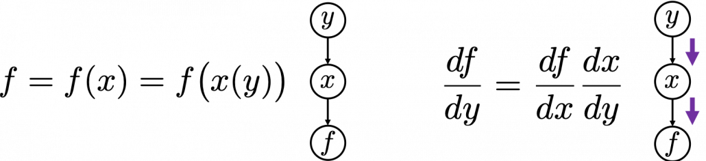
First, let’s think about the simplest type of chain rule. Assume that you have a function $f=f(x)=f(x(y))$ , and relations of the functions are displayed as the graphical model at the left side of the figure below. Variables are a type of function, so you should think that every node in graphical models denotes a function. Arrows in purple in the right side of the chart show how information propagate in differentiation.

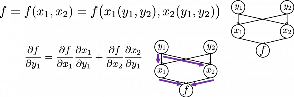
Next, if you have a function $f$ , which has two variances $x_1$ and $x_2$ . And both of the variances also share two variances $y_1$ and $y_2$ . When you take partial differentiation of $f$ with respect to $y_1$ or $y_2$ , the formula is a little tricky. Let’s think about how to calculate $\frac{\partial f}{\partial y_1}$ . The variance $y_1$ propagates to $f$ via $x_1$ and $x_2$ . In this case the partial differentiation has two terms as below.

In chain rules, you have to think about all the routes where a variance can propagate through. If you generalize chain rules as the graphical model below, the partial differentiation of $f$ with respect to $y_i$ is calculated as below. And you need to understand chain rules in this way to understanding any types of back propagation.

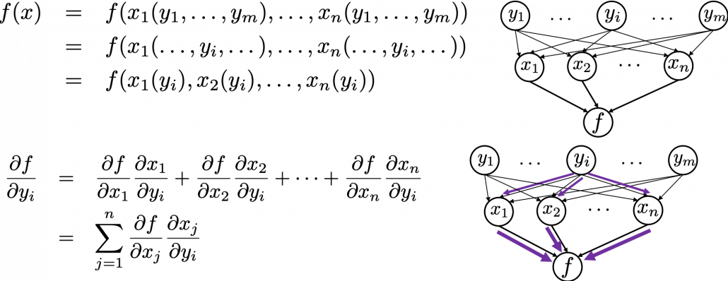
The figure above shows that if you calculate partial differentiation of $f$ with respect to $y_i$ , the partial differentiation has $n$ terms in total because $y_i$ propagates to $f$ via $n$ variances. In order to understand backprop of LSTM, you constantly have to care about the flows of variances, which I display as purple arrows.

2. Chain rules in LSTM

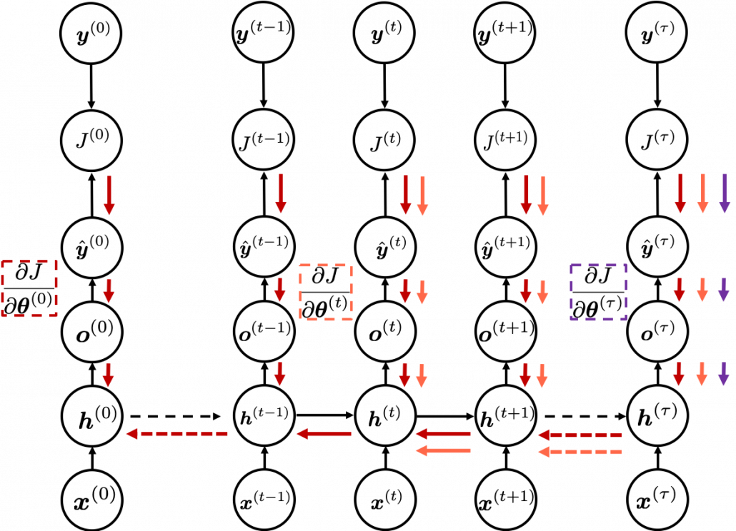
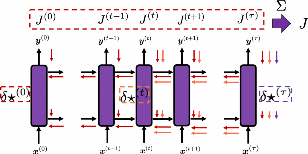
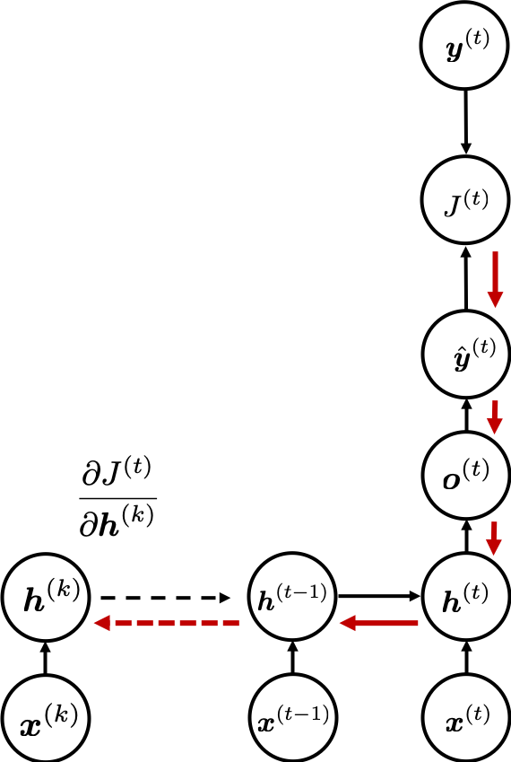
I would like you to remember the figure below, which I used in the second article to show how errors propagate backward during backprop of simple RNNs. After forward propagation, first of all, you need to calculate $\frac{\partial J}{\partial \boldsymbol{\theta}^{(t)}}$ , gradients of the error function with respect to parameters, at each time step. But you have to be careful that even though these gradients depend on time steps, the parameters $\boldsymbol{\theta}$ do not depend on time steps.

*As I mentioned in the second article I personally think $\frac{\partial J}{\partial \boldsymbol{\theta}^{(t)}}$ should be rather denoted as $(\frac{\partial J}{\partial \boldsymbol{\theta}})^{(t)}$ because parameters themselves do not depend on time. However even the textbook by MIT press partly use the former notation. And I think you are likely to encounter this type of notation, so I think it is not bad to get ready for both.

The errors at time step $(t)$ propagate backward to all the $\boldsymbol{h} ^{(s)} (s \leq t)$ . Conversely, in order to calculate $\frac{\partial J}{\partial \boldsymbol{\theta}^{(t)}}$ errors flowing from $J^{(s)} (s \geq t)$ . In the chart you need arrows of errors in purple for the gradient in a purple frame, orange arrows for gradients in orange frame, red arrows for gradients in red frame. And you need to sum up $\frac{\partial J}{\partial \boldsymbol{\theta}^{(t)}}$ to calculate $\frac{\partial J}{\partial \boldsymbol{\theta}} = \sum_{t}{\frac{\partial J}{\partial \boldsymbol{\theta}^{(t)}}}$ , and you need this gradient $\frac{\partial J}{\partial \boldsymbol{\theta}}$ to renew parameters, one time.

At an RNN block level, the flows of errors and how to renew parameters are the same in LSTM backprop, but the flow of errors inside each block is much more complicated in LSTM backprop. But in order to denote errors of LSTM backprop, instead of $\frac{\partial J}{\partial \boldsymbol{\theta}^{(t)}}$ , I use a special notation $\delta \star ^{(t)} = \frac{\partial J}{\partial \star}$ .

* Again, please be careful of what $\delta \star ^{(t)}$ means. Neurons depend on time steps, but parameters do not depend on time steps. So if $\star$ are neurons, $\delta \star ^{(t)}= \frac{\partial J}{ \partial \star ^{(t)}}$ , but when $\star$ are parameters, $\delta \star ^{(t)}$ should be rather denoted like $\delta \star ^{(t)}= (\frac{\partial J}{ \partial \star })^{(t)}$ . In the Space Odyssey paper, $\boldsymbol{\star}$ are not used as parameters, but in my PowerPoint slides and some other materials, $\boldsymbol{\star}$ are used also as parameteres.

As I wrote in the last article, you calculate $\boldsymbol{f}^{(t)}, \boldsymbol{i}^{(t)}, \boldsymbol{z}^{(t)}, \boldsymbol{o}^{(t)}$ as below. Unlike the last article, I also added the terms of peephole connections in the equations below, and I also introduced the variances $\bar{\boldsymbol{f}}^{(t)}, \bar{\boldsymbol{i}}^{(t)}, \bar{\boldsymbol{z}}^{(t)}, \bar{\boldsymbol{o}}^{(t)}$ for convenience.

$\boldsymbol{\bar{f}}^{(t)}=\boldsymbol{W}_{for} \cdot \boldsymbol{x}^{(t)} + \boldsymbol{R}_{for} \cdot \boldsymbol{y}^{(t-1)} + \boldsymbol{p}_{for}\odot \boldsymbol{c}^{(t-1)} + \boldsymbol{b}_{for}$
$\boldsymbol{\bar{i}}^{(t)}=\boldsymbol{W}_{in} \cdot \boldsymbol{x}^{(t)} + \boldsymbol{R}_{in} \cdot \boldsymbol{y}^{(t-1)} + \boldsymbol{p}_{in}\odot \boldsymbol{c}^{(t-1)} + \boldsymbol{b}_{in}$
$\boldsymbol{\bar{z}}^{(t)}=\boldsymbol{W}_z \cdot \boldsymbol{x}^{(t)} + \boldsymbol{R}_z \cdot \boldsymbol{y}^{(t-1)} + \boldsymbol{b}_z$
$\boldsymbol{\bar{o}}^{(t)}=\boldsymbol{W}_{out} \cdot \boldsymbol{x}^{(t)} + \boldsymbol{R}_{out} \cdot \boldsymbol{y}^{(t-1)} + \boldsymbol{p}_{out}\odot \boldsymbol{c}^{(t)} + \boldsymbol{b}_{out}$
$\boldsymbol{f}^{(t)}=\sigma( \boldsymbol{\bar{f}}^{(t)})$
$\boldsymbol{i}^{(t)}=\sigma(\boldsymbol{\bar{i}}^{(t)})$
$\boldsymbol{z}^{(t)}=tanh(\boldsymbol{\bar{z}}^{(t)})$
$\boldsymbol{o}^{(t)}=\sigma(\boldsymbol{\bar{o}}^{(t)})$

With Hadamar product operator, the renewed cell and the output are calculated as below.

$\boldsymbol{c}^{(t)} = \boldsymbol{z}^{(t)}\odot \boldsymbol{i}^{(t)} + \boldsymbol{c}^{(t-1)} \odot \boldsymbol{f}^{(t)}$
$\boldsymbol{y}^{(t)} = \boldsymbol{o}^{(t)} \odot tanh(\boldsymbol{c}^{(t)})$

In this article I would rather give instructions on how to read my PowerPoint slide. Just as general backprop, you need to calculate gradients of error functions with respect to parameters, such as $\delta \boldsymbol{W}_{\star}, \delta \boldsymbol{R}_{\star}, \delta \boldsymbol{p}_{\star}, \delta \boldsymbol{b}_{\star}$ , where $\star$ is either of $\{z, in, for, out \}$ . And just as backprop of simple RNNs, in order to calculate gradients with respect to parameters, you need to calculate errors of neurons, that is gradients of error functions with respect to neurons, such as $\delta \boldsymbol{f}^{(t)}, \delta \boldsymbol{i}^{(t)}, \delta \boldsymbol{z}^{(t)}, \delta \boldsymbol{o}^{(t)}$ .

*Again and again, keep it in mind that neurons depend on time steps, but parameters do not depend on time steps.

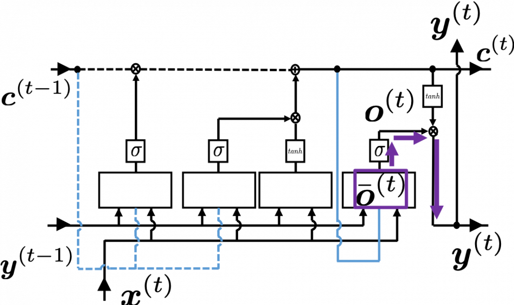
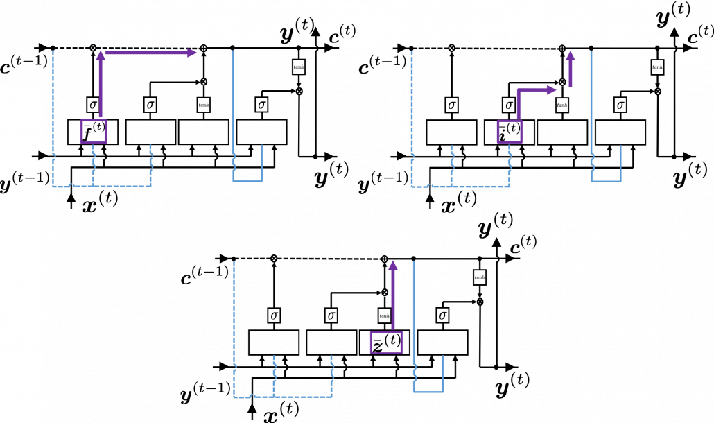
When you calculate gradients with respect to neurons, you can first calculate $\delta \boldsymbol{y}^{(t)}$ , but the equation for this error is the most difficult, so I recommend you to put it aside for now. After calculating $\delta \boldsymbol{y}^{(t)}$ , you can next calculate $\delta \bar{\boldsymbol{o}}^{(t)}= \frac{\partial J^{(t)}}{ \partial \bar{\boldsymbol{o}}^{(t)}}$ . If you see the LSTM block below as a graphical model which I introduced, the information of $\bar{\boldsymbol{o}}^{(t)}$ flow like the purple arrows. That means, $\bar{\boldsymbol{o}}^{(t)}$ affects $J$ only via $\boldsymbol{y}^{(t)}$ , and this structure is equal to the first graphical model which I have introduced above. And if you calculate $\bar{\boldsymbol{o}}^{(t)}$ element-wise, you get the equation $\delta \bar{o}_{k}^{(t)}=\frac{\partial J}{\partial \bar{o}_{k}^{(t)}}= \frac{\partial J}{\partial y_{k}^{(t)}} \frac{\partial y_{k}^{(t)}}{\partial \bar{o}_{k}^{(t)}}$ .

*The $k$ is an index of an element of vectors. If you can calculate element-wise gradients, it is easy to understand that as differentiation of vectors and matrices.

Next you can calculate $\delta \boldsymbol{c}^{(t)}$ , and chain rules are very important in this process. The flow of $\delta \boldsymbol{c}^{(t)}$ to $J$ can be roughly divided into two streams: the one which flows to $J$ as $\bodlsymbol{y}^{(t)}$ , and the one which flows to $J$ as $\bodlsymbol{c}^{(t+1)}$ . And the stream from $\bodlsymbol{c}^{(t)}$ to $\bodlsymbol{y}^{(t)}$ also have two branches: the one via $\bar{\boldsymbol{o}}^{(t)}$ and the one which directly converges as $\bodlsymbol{y}^{(t)}$ . Just as well, the stream from $\bodlsymbol{c}^{(t)}$ to $\bodlsymbol{c}^{(t+1)}$ also have three branches: the ones via $\bar{\boldsymbol{f}}^{(t)}$ , $\bar{\boldsymbol{i}}^{(t)}$ , and the one which directly converges as $\bodlsymbol{c}^{(t+1)}$ .

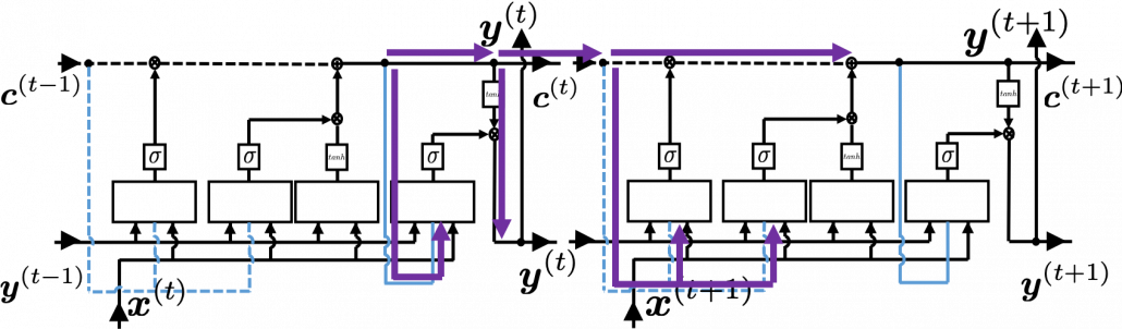
If you see see these flows as graphical a graphical model, that would be like the figure below.

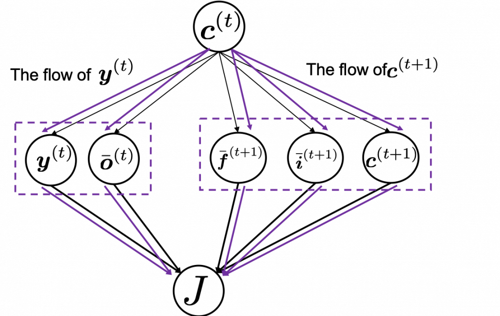
According to this graphical model, you can calculate $\delta \boldsymbol{c} ^{(t)}$ element-wise as below.

* TO BE VERY HONEST I still do not fully understand why we can apply chain rules like above to calculate $\delta \boldsymbol{c}^{(t)}$ . When you apply the formula of chain rules, which I showed in the first section, to this case, you have to be careful of where to apply partial differential operators $\frac{\partial}{ \partial c_{k}^{(t)}}$ . In the case above, in the part $\frac{\partial y_{k}^{(t)}}{\partial c_{k}^{(t)}}$ the partial differential operator only affects $tanh(c_{k}^{(t)})$ of $o_{k}^{(t)} \cdot tanh(c_{k}^{(t)})$ . And in the part $\frac{\partial c_{k}^{(t+1)}}{\partial c_{k}^{(t)}}$ , the partial differential operator $\frac{\partial}{\partial c_{k}^{(t)}}$ only affects the part $c_{k}^{(t)}$ of the term $c^{t}_{k} \cdot f_{k}^{(t+1)}$ . In the $\frac{\partial \bar{o}_{k}^{(t)}}{\partial c_{k}^{(t)}}$ part, only $(p_{out})_{k} \cdot c_{k}^{(t)}$ , in the $\frac{\partial \bar{i}_{k}^{(t+1)}}{\partial c_{k}^{(t)}}$ part, only $(p_{in})_{k} \cdot c_{k}^{(t)}$ , and in the $\frac{\partial \bar{f}_{k}^{(t+1)}}{\partial c_{k}^{(t)}}$ part, only $(p_{in})_{k} \cdot c_{k}^{(t)}$ . But some other parts, which are not affected by $\frac{\partial}{ \partial c_{k}^{(t)}}$ are also functions of $c_{k}^{(t)}$ . For example $o_{k}^{(t)}$ of $o_{k}^{(t)} \cdot tanh(c_{k}^{(t)})$ is also a function of $c_{k}^{(t)}$ . And I am still not sure about the logic behind where to affect those partial differential operators.

*But at least, these are the only decent equations for LSTM backprop which I could find, and a frequently cited paper on LSTM uses implementation based on these equations. Computer science is more of practical skills, rather than rigid mathematical logic. Also I think I have spent great deal of my time thinking about this part, and it is now time for me to move to next step. If you have any comments or advice on this point, please let me know.

Calculating $\delta \bar{\boldsymbol{f}}^{(t)}$ , $\delta \bar{\boldsymbol{i}}^{(t)}$ , $\delta \bar{\boldsymbol{z}}^{(t)}$ are also relatively straigtforward as calculating $\delta \bar{\boldsymbol{o}}^{(t)}$ . They all use the first type of chain rule in the first section. Thereby you can get these gradients: $\delta \bar{f}_{k}^{(t)}=\frac{\partial J}{ \partial \bar{f}_{k}^{(t)}} =\frac{\partial J}{\partial c_{k}^{(t)}} \frac{\partial c_{k}^{(t)}}{ \partial \bar{f}_{k}^{(t)}}$ , $\delta \bar{i}_{k}^{(t)}=\frac{\partial J}{\partial \bar{i}_{k}^{(t)}} =\frac{\partial J}{\partial c_{k}^{(t)}} \frac{\partial c_{k}^{(t)}}{ \partial \bar{i}_{k}^{(t)}}$ , and $\delta \bar{z}_{k}^{(t)}=\frac{\partial J}{\partial \bar{z}_{k}^{(t)}} =\frac{\partial J}{\partial c_{k}^{(t)}} \frac{\partial c_{k}^{(t)}}{ \partial \bar{i}_{k}^{(t)}}$ .

All the gradients which we have calculated use the error $\delta \boldsymbol{y}^{(t)}$ , but when it comes to calculating $\delta \boldsymbol{y}^{(t)}$ ….. I can only say “Please be patient. I did my best in my PowerPoint slides to explain that.” It is not a kind of process which I want to explain on Word Press. In conclusion you get an error like this: $\delta \boldsymbol{y}^{(t)}=\frac{\partial J^{(t)}}{\partial \boldsymbol{y}^{(t)}} + \boldsymbol{R}_{for}^{T} \delta \bar{\boldsymbol{f}}^{(t+1)} + \boldsymbol{R}_{in}^{T}\delta \bar{\boldsymbol{i}}^{(t+1)} + \boldsymbol{R}_{out}^{T}\delta \bar{\boldsymbol{o}}^{(t+1)} + \boldsymbol{R}_{z}^{T}\delta \bar{\boldsymbol{z}}^{(t+1)}$ , and the flows of $\boldsymbol{y}^{(t)}$ are as blow.

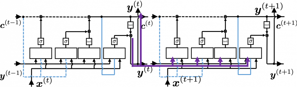
Combining the gradients we have got so far, we can calculate gradients with respect to parameters. For concrete results, please check the Space Odyssey paper or my PowerPoint slide.

3. How LSTMs tackle exploding/vanishing gradients problems

*If you are allergic to mathematics, you should not read this section or even download my PowerPoint slide.

*Part of this section is more or less subjective, so if you really want to know how LSTM mitigate the problems, I highly recommend you to also refer to other materials. But at least I did my best for this article.

LSTMs do not completely solve, vanishing gradient problems. They mitigate vanishing/exploding gradient problems. I am going to roughly explain why they can tackle those problems. I think you find many explanations on that topic, but many of them seems to have some mathematical mistakes (even the slide used in a lecture in Stanford University) and I could not partly agree with some statements. I also could not find any papers or materials which show the whole picture of how LSTMs can tackle those problems. So in this article I am only going to give instructions on the major way to explain this topic.

First let’s see how gradients actually “vanish” or “explode” in simple RNNs. As I in the second article of this series, simple RNNs propagate forward as the equations below.

$\boldsymbol{a}^{(t)} = \boldsymbol{b} + \boldsymbol{W} \cdot \boldsymbol{h}^{(t-1)} + \boldsymbol{U} \cdot \boldsymbol{x}^{(t)}$
$\boldsymbol{h}^{(t)}= g(\boldsymbol{a}^{(t)})$
$\boldsymbol{o}^{(t)} = \boldsymbol{c} + \boldsymbol{V} \cdot \boldsymbol{h}^{(t)}$
$\hat{\boldsymbol{y}} ^{(t)} = f(\boldsymbol{o}^{(t)})$

And every time step, you get an error function $J^{(t)}$ . Let’s consider the gradient of $J^{(t)}$ with respect to $\boldsymbol{h}^{(k)}$ , that is the error flowing from $J^{(t)}$ to $\boldsymbol{h}^{(k)}$ . This error is the most used to calculate gradients of the parameters in the equations above.

If you calculate this error more concretely, $\frac{\partial J^{(t)}}{\partial \boldsymbol{h}^{(k)}} = \frac{\partial J^{(t)}}{\partial \boldsymbol{h}^{(t)}} \frac{\partial \boldsymbol{h}^{(t)}}{\partial \boldsymbol{h}^{(t-1)}} \cdots \frac{\partial \boldsymbol{h}^{(k+2)}}{\partial \boldsymbol{h}^{(k+1)}} \frac{\partial \boldsymbol{h}^{(k+1)}}{\partial \boldsymbol{h}^{(k)}} = \frac{\partial J^{(t)}}{\partial \boldsymbol{h}^{(t)}} \prod_{k< s \leq t} \frac{\partial \boldsymbol{h}^{(s)}}{\partial \boldsymbol{h}^{(s-1)}}$ , where $\frac{\partial \boldsymbol{h}^{(s)}}{\partial \boldsymbol{h}^{(s-1)}} = \boldsymbol{W} ^T \cdot diag(g'(\boldsymbol{b} + \boldsymbol{W}\cdot \boldsymbol{h}^{(s-1)} + \boldsymbol{U}\cdot \boldsymbol{x}^{(s)})) = \boldsymbol{W} ^T \cdot diag(g'(\boldsymbol{a}^{(s)}))$ .

* If you see the figure as a type of graphical model, you should be able to understand the why chain rules can be applied as the equation above.

*According to this paper $\frac{\partial \boldsymbol{h}^{(s)}}{\partial \boldsymbol{h}^{(s-1)}} = \boldsymbol{W} ^T \cdot diag(g'(\boldsymbol{a}^{(s)}))$ , but it seems that many study materials and web sites are mistaken in this point.

Hence $\frac{\partial J^{(t)}}{\partial \boldsymbol{h}^{(k)}} = \frac{\partial J^{(t)}}{\partial \boldsymbol{h}^{(t)}} \prod_{k< s \leq t} \boldsymbol{W} ^T \cdot diag(g'(\boldsymbol{a}^{(s)})) = \frac{\partial J^{(t)}}{\partial \boldsymbol{h}^{(t)}} (\boldsymbol{W} ^T )^{(t - k)} \prod_{k< s \leq t} diag(g'(\boldsymbol{a}^{(s)}))$ . If you take norms of $\frac{\partial J^{(t)}}{\partial \boldsymbol{h}^{(k)}}$ you get an equality $\left\lVert \frac{\partial J^{(t)}}{\partial \boldsymbol{h}^{(k)}} \right\rVert \leq \left\lVert \frac{\partial J^{(t)}}{\partial \boldsymbol{h}^{(t)}} \right\rVert \left\lVert \boldsymbol{W} ^T \right\rVert ^{(t - k)} \prod_{k< s \leq t} \left\lVert diag(g'(\boldsymbol{a}^{(s)}))\right\rVert$ . I will not go into detail anymore, but it is known that according to this inequality, multiplication of weight vectors exponentially converge to 0 or to infinite number.

We have seen that the error $\frac{\partial J^{(t)}}{\partial \boldsymbol{h}^{(k)}}$ is the main factor causing vanishing/exploding gradient problems of simple RNNs. In case of LSTM, $\frac{\partial J^{(t)}}{\partial \boldsymbol{c}^{(k)}}$ is an equivalent. For simplicity, let’s calculate only $\frac{\partial \boldsymbol{c}^{(t)}}{\partial \boldsymbol{c}^{(t-1)}}$ , which is equivalent to $\frac{\partial \boldsymbol{h}^{(t)}}{\partial \boldsymbol{h}^{(t-1)}}$ of simple RNN backprop.

* Just as I noted above, you have to be careful of which part the partial differential operator $\frac{\partial}{\partial \boldsymbol{c}^{(t-1)}}$ affects in the chain rule above. That is, you need to calculate $\frac{\partial}{\partial \boldsymbol{c}^{(t-1)}} (\boldsymbol{c}^{(t-1)} \odot \boldsymbol{f}^{(t)})$ , and the partial differential operator only affects $\boldsymbol{c}^{(t-1)}$ . I think this is not a correct mathematical notation, but please forgive me for doing this for convenience.

If you continue calculating the equation above more concretely, you get the equation below.

I cannot mathematically explain why, but it is known that this characteristic of gradients of LSTM backprop mitigate the vanishing/exploding gradient problem. We have seen that if you take a norm of $\frac{\partial J^{(t)}}{\partial \boldsymbol{h}^{(k)}}$ , that is equal or smaller than repeated multiplication of the norm of the same weight matrix, and that soon leads to vanishing/exploding gradient problem. But according to the equation above, even if you take a norm of repeatedly multiplied $\frac{\partial \boldsymbol{c}^{(t)}}{\partial \boldsymbol{c}^{(t-1)}}$ , its norm cannot be evaluated with a simple value like repeated multiplication of the norm of the same weight matrix. The outputs of each gate are different from time steps to time steps, and that adjust the value of $\frac{\partial \boldsymbol{c}^{(t)}}{\partial \boldsymbol{c}^{(t-1)}}$ .

*I personally guess the term $diag(\boldsymbol{f}^{(t)})$ is very effective. The unaffected value of the elements of $\boldsymbol{f}^{(t)}$ can directly adjust the value of $\frac{\partial \boldsymbol{c}^{(t)}}{\partial \boldsymbol{c}^{(t-1)}}$ . And as a matter of fact, it is known that performances of LSTM drop the most when you get rid of forget gates.

When it comes to tackling exploding gradient problems, there is a much easier technique called gradient clipping. This algorithm is very simple: you just have to adjust the size of gradient so that the absolute value of gradient is under a threshold at every time step. Imagine that you decide in which direction to move by calculating gradients, but when the footstep is going to be too big, you just adjust the size of footstep to the threshold size you have set. In a pseudo code, you can write a gradient clipping part only with some two line codes as below.

* $\boldsymbol{g}$ is a gradient at the time step $threshold$ is the maximum size of the “step.”

The figure below, cited from a deep learning text from MIT press textbook, is a good and straightforward explanation on gradient clipping.It is known that a strongly nonlinear function, such as error functions of RNN, can have very steep or plain areas. If you artificially visualize the idea in 3-dimensional space, as the surface of a loss function $J$ with two variants $w, b$ , that means the loss function $J$ has plain areas and very steep cliffs like in the figure.Without gradient clipping, at the left side, you can see that the black dot all of a sudden climb the cliff and could jump to an unexpected area. But with gradient clipping, you avoid such “big jumps” on error functions.

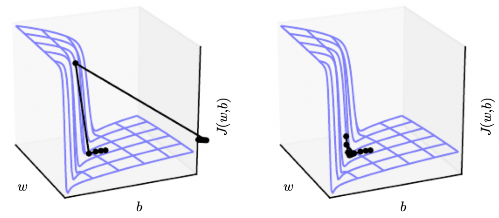
Source: Source: Goodfellow and Yoshua Bengio and Aaron Courville, Deep Learning, (2016), MIT Press, 409p

I am glad that I have finally finished this article series. I am not sure how many of the readers would have read through all of the articles in this series, including my PowerPoint slides. I bet that is not so many. I spent a great deal of my time for making these contents, but sadly even when I was studying LSTM, it was becoming old-fashioned, at least in natural language processing (NLP) field: a very promising algorithm named Transformer has been replacing the position of LSTM. Deep learning is a very fast changing field. I also would like to make illustrative introductions on attention mechanism in NLP, from seq2seq model to Transformer. And I think LSTM would still remain as one of the algorithms in sequence data processing, such as hidden Hidden Markov model, or particle filter.

* I make study materials on machine learning, sponsored by DATANOMIQ. I do my best to make my content as straightforward but as precise as possible. I include all of my reference sources. If you notice any mistakes in my materials, including grammatical errors, please let me know (email: yasuto.tamura@datanomiq.de). And if you have any advice for making my materials more understandable to learners, I would appreciate hearing it.