Data-driven Attribution Modeling
/in Artificial Intelligence, Business Analytics, Business Intelligence, Data Science, Deep Learning, Machine Learning, Main Category, Use Cases/by Alexander LammersIn the world of commerce, companies often face the temptation to reduce their marketing spending, especially during times of economic uncertainty or when planning to cut costs. However, this short-term strategy can lead to long-term consequences that may hinder a company’s growth and competitiveness in the market.
Maintaining a consistent marketing presence is crucial for businesses, as it helps to keep the company at the forefront of their target audience’s minds. By reducing marketing efforts, companies risk losing visibility and brand awareness among potential clients, which can be difficult and expensive to regain later. Moreover, a strong marketing strategy is essential for building trust and credibility with prospective customers, as it demonstrates the company’s expertise, values, and commitment to their industry.
Given a fixed budget, companies apply economic principles for marketing efforts and need to spend a given marketing budget as efficient as possible. In this view, attribution models are an essential tool for companies to understand the effectiveness of their marketing efforts and optimize their strategies for maximum return on investments (ROI). By assigning optimal credit to various touchpoints in the customer journey, these models provide valuable insights into which channels, campaigns, and interactions have the greatest impact on driving conversions and therefore revenue. Identifying the most important channels enables companies to distribute the given budget accordingly in an optimal way.
1. Combining business value with attribution modeling
The true value of attribution modeling lies not solely in applying the optimal theoretical concept – that are discussed below – but in the practical application in coherence with the business logic of the firm. Therefore, the correct modeling ensures that companies are not only distributing their budget in an optimal way but also that they incorporate the business logic to focus on an optimal long-term growth strategy.
Understanding and incorporating business logic into attribution models is the critical step that is often overlooked or poorly understood. However, it is the key to unlocking the full potential of attribution modeling and making data-driven decisions that align with business goals. Without properly integrating the business logic, even the most sophisticated attribution models will fail to provide actionable insights and may lead to misguided marketing strategies.
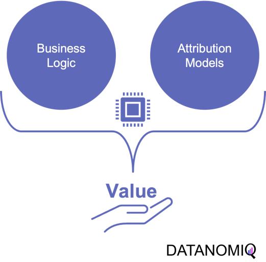
Figure 1 – Combining the business logic with attribution modeling to generate value for firms
For example, determining the end of a customer journey is a critical step in attribution modeling. When there are long gaps between customer interactions and touchpoints, analysts must carefully examine the data to decide if the current journey has concluded or is still ongoing. To make this determination, they need to consider the length of the gap in relation to typical journey durations and assess whether the gap follows a common sequence of touchpoints. By analyzing this data in an appropriate way, businesses can more accurately assess the impact of their marketing efforts and avoid attributing credit to touchpoints that are no longer relevant.
Another important consideration is accounting for conversions that ultimately lead to returns or cancellations. While it’s easy to get excited about the number of conversions generated by marketing campaigns, it’s essential to recognize that not all conversions should be valued equal. If a significant portion of conversions result in returns or cancellations, the true value of those campaigns may be much lower than initially believed.
To effectively incorporate these factors into attribution models, businesses need to important things. First, a robust data platform (such as a customer data platform; CDP) that can integrate data from various sources, such as tracking systems, ERP systems, e-commerce platforms to effectively perform data analytics. This allows for a holistic view of the customer journey, including post-conversion events like returns and cancellations, which are crucial for accurate attribution modeling. Second, as outlined above, businesses need a profound understanding of the business model and logic.
2. On the Relevance of Attribution Models in Online Marketing
A conversion is a point in the customer journey where a recipient of a marketing message performs a somewhat desired action. For example, open an email, click on a call-to-action link or go to a landing page and fill out a registration. Finally, the ultimate conversion would be of course buying the product. Attribution models serve as frameworks that help marketers assess the business impact of different channels on a customer’s decision to convert along a customer´s journey. By providing insights into which interactions most effectively drive sales, these models enable more efficient resource allocation given a fixed budget.

Figure 2 – A simple illustration of one single customer journey. Consider that from the company’s perspective all journeys together result into a complex network of possible journey steps.
Companies typically utilize a diverse marketing mix, including email marketing, search engine advertising (SEA), search engine optimization (SEO), affiliate marketing, and social media. Attribution models facilitate the analysis of customer interactions across these touchpoints, offering a comprehensive view of the customer journey.
-
Comprehensive Customer Insights: By identifying the most effective channels for driving conversions, attribution models allow marketers to tailor strategies that enhance customer engagement and improve conversion rates.
-
Optimized Budget Allocation: These models reveal the performance of various marketing channels, helping marketers allocate budgets more efficiently. This ensures that resources are directed towards channels that offer the highest return on investment (ROI), maximizing marketing impact.
-
Data-Driven Decision Making: Attribution models empower marketers to make informed, data-driven decisions, leading to more effective campaign strategies and better alignment between marketing and sales efforts.
In the realm of online advertising, evaluating media effectiveness is a critical component of the decision-making process. Since advertisement costs often depend on clicks or impressions, understanding each channel’s effectiveness is vital. A multi-channel attribution model is necessary to grasp the marketing impact of each channel and the overall effectiveness of online marketing activities. This approach ensures optimal budget allocation, enhances ROI, and drives successful marketing outcomes.
What types of attribution models are there? Depending on the attribution model, different values are assigned to various touchpoints. These models help determine which channels are the most important and should be prioritized. Each channel is assigned a monetary value based on its contribution to success. This weighting then determines the allocation of the marketing budget. Below are some attribution models commonly used in marketing practice.
2.1. Single-Touch Attribution Models
As it follows from the name of the group of these approaches, they consider only one touchpoint.
2.1.1 First Touch Attribution
First touch attribution is the standard and simplest method for attributing conversions, as it assigns full credit to the first interaction. One of its main advantages is its simplicity; it is a straightforward and easy-to-understand approach. Additionally, it allows for quick implementation without the need for complex calculations or data analysis, making it a convenient choice for organizations looking for a simple attribution method. This model can be particularly beneficial when the focus is solely on demand generation. However, there are notable drawbacks to first touch attribution. It tends to oversimplify the customer journey by ignoring the influence of subsequent touchpoints. This can lead to a limited view of channel performance, as it may disproportionately credit channels that are more likely to be the first point of contact, potentially overlooking the contributions of other channels that assist in conversions.
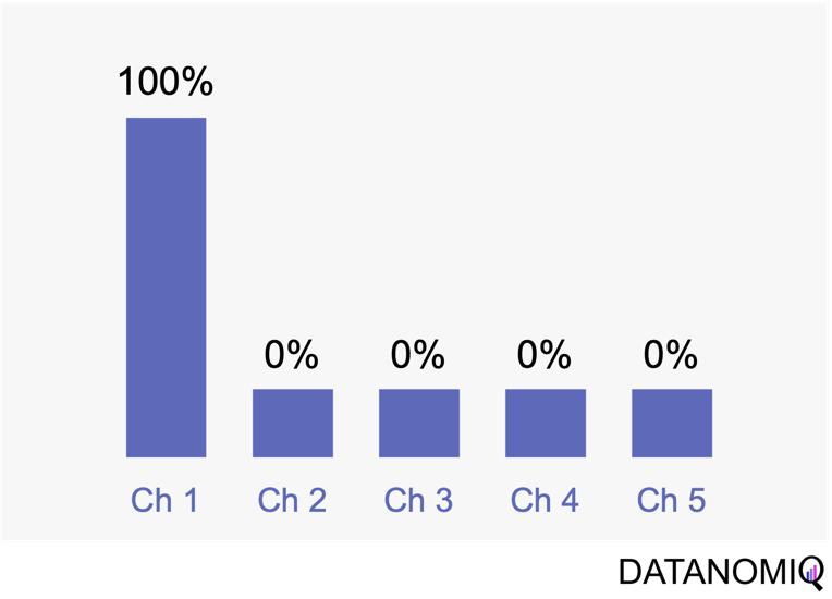
Figure 3 – The first touch is a simple non-intelligent way of attribution.
2.1.2 Last Touch Attribution
Last touch attribution is another straightforward method for attributing conversions, serving as the opposite of first touch attribution by assigning full credit to the last interaction. Its simplicity is one of its main advantages, as it is easy to understand and implement without the need for complex calculations or data analysis. This makes it a convenient choice for organizations seeking a simple attribution approach, especially when the focus is solely on driving conversions. However, last touch attribution also has its drawbacks. It tends to oversimplify the customer journey by neglecting the influence of earlier touchpoints. This approach provides limited insights into the full customer journey, as it focuses solely on the last touchpoint and overlooks the cumulative impact of multiple touchpoints, missing out on valuable insights.
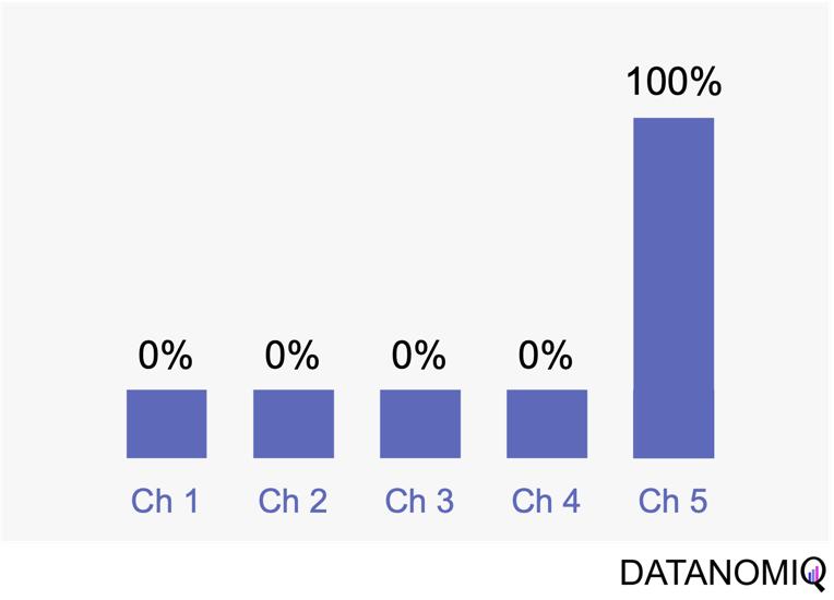
Figure 4 – Last touch attribution is the counterpart to the first touch approach.
2.2 Multi-Touch Attribution Models
We noted that single-touch attribution models are easy to interpret and implement. However, these methods often fall short in assigning credit, as they apply rules arbitrarily and fail to accurately gauge the contribution of each touchpoint in the consumer journey. As a result, marketers may make decisions based on skewed data. In contrast, multi-touch attribution leverages individual user-level data from various channels. It calculates and assigns credit to the marketing touchpoints that have influenced a desired business outcome for a specific key performance indicator (KPI) event.
2.2.1 Linear Attribution
Linear attribution is a standard approach that improves upon single-touch models by considering all interactions and assigning them equal weight. For instance, if there are five touchpoints in a customer’s journey, each would receive 20% of the credit for the conversion. This method offers several advantages. Firstly, it ensures equal distribution of credit across all touchpoints, providing a balanced representation of each touchpoint’s contribution to conversions. This approach promotes fairness by avoiding the overemphasis or neglect of specific touchpoints, ensuring that credit is distributed evenly among channels. Additionally, linear attribution is easy to implement, requiring no complex calculations or data analysis, which makes it a convenient choice for organizations seeking a straightforward attribution method. However, linear attribution also has its drawbacks. One significant limitation is its lack of differentiation, as it assigns equal credit to each touchpoint regardless of their actual impact on driving conversions. This can lead to an inaccurate representation of the effectiveness of individual touchpoints. Furthermore, linear attribution ignores the concept of time decay, meaning it does not account for the diminishing influence of earlier touchpoints over time. It treats all touchpoints equally, regardless of their temporal proximity to the conversion event, potentially overlooking the greater impact of more recent interactions.
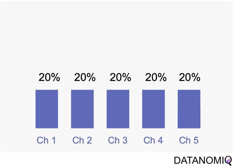
Figure 5 – Linear uniform attribution.
2.2.2 Position-based Attribution (U-Shaped Attribution & W-Shaped Attribution)
Position-based attribution, encompassing both U-shaped and W-shaped models, focuses on assigning the most significant weight to the first and last touchpoints in a customer’s journey. In the W-shaped attribution model, the middle touchpoint also receives a substantial amount of credit. This approach offers several advantages. One of the primary benefits is the weighted credit system, which assigns more credit to key touchpoints such as the first and last interactions, and sometimes additional key touchpoints in between. This allows marketers to highlight the importance of these critical interactions in driving conversions. Additionally, position-based attribution provides flexibility, enabling businesses to customize and adjust the distribution of credit according to their specific objectives and customer behavior patterns. However, there are some drawbacks to consider. Position-based attribution involves a degree of subjectivity, as determining the specific weights for different touchpoints requires subjective decision-making. The choice of weights can vary across organizations and may affect the accuracy of the attribution results. Furthermore, this model has limited adaptability, as it may not fully capture the nuances of every customer journey, given its focus on specific positions or touchpoints.
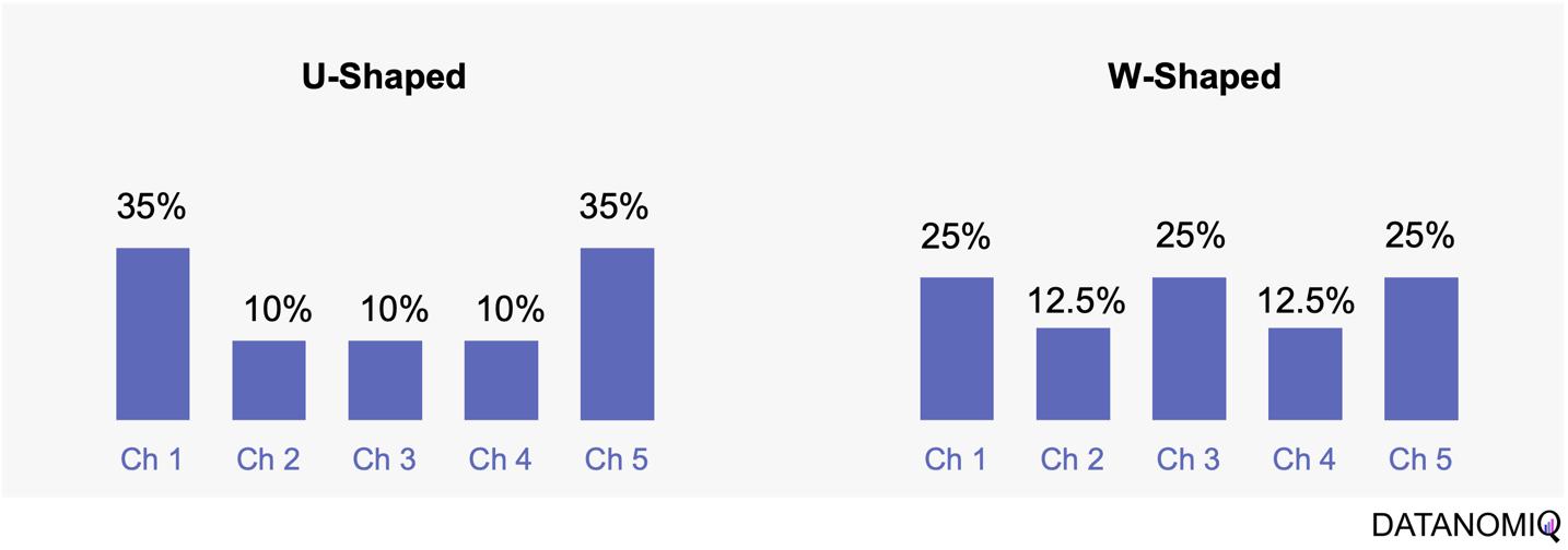
Figure 6 – The U-shaped attribution (sometimes known as “bathtube model” and the W-shaped one are first attempts of weighted models.
2.2.3 Time Decay Attribution
Time decay attribution is a model that primarily assigns most of the credit to interactions that occur closest to the point of conversion. This approach has several advantages. One of its key benefits is temporal sensitivity, as it recognizes the diminishing impact of earlier touchpoints over time. By assigning more credit to touchpoints closer to the conversion event, it reflects the higher influence of recent interactions. Additionally, time decay attribution offers flexibility, allowing organizations to customize the decay rate or function. This enables businesses to fine-tune the model according to their specific needs and customer behavior patterns, which can be particularly useful for fast-moving consumer goods (FMCG) companies. However, time decay attribution also has its drawbacks. One challenge is the arbitrary nature of the decay function, as determining the appropriate decay rate is both challenging and subjective. There is no universally optimal decay function, and choosing an inappropriate model can lead to inaccurate credit distribution. Moreover, this approach may oversimplify time dynamics by assuming a linear or exponential decay pattern, which might not fully capture the complex temporal dynamics of customer behavior. Additionally, time decay attribution primarily focuses on the temporal aspect and may overlook other contextual factors that influence touchpoint effectiveness, such as channel interactions, customer segments, or campaign-specific dynamics.
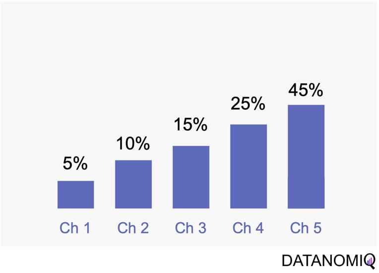
Figure 7 – Time-based models can be configurated by according to the first or last touch and weighted by the timespan in between of each touchpoint.
2.3 Data-Driven Attribution Models
2.3.1 Markov Chain Attribution
Markov chain attribution is a data-driven method that analyzes marketing effectiveness using the principles of Markov Chains. Those chains are mathematical models used to describe systems that transition from one state to another in a chain-like process. The principles focus on the transition matrix, derived from analyzing customer journeys from initial touchpoints to conversion or no conversion, to capture the sequential nature of interactions and understand how each touchpoint influences the final decision. Let’s have a look at the following simple example with three channels that are chained together and leading to either a conversion or no conversion.
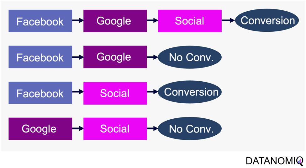
Figure 8 – Example of four customer journeys
The model calculates the conversion likelihood by examining transitions between touchpoints. Those transitions are depicted in the following probability tree.
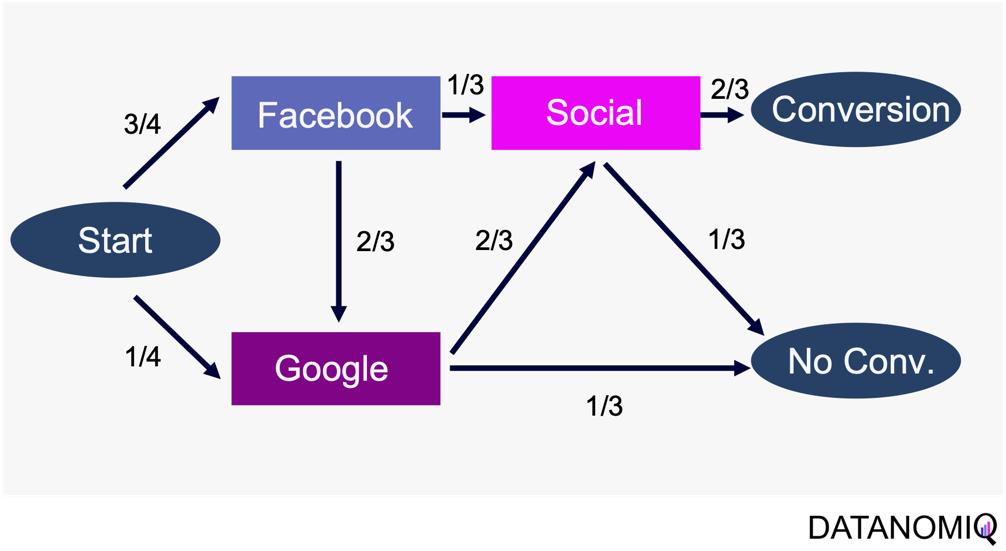
Figure 9 – Example of a touchpoint network based on customer journeys
Based on this tree, the transition matrix can be constructed that reveals the influence of each touchpoint and thus the significance of each channel.
This method considers the sequential nature of customer journeys and relies on historical data to estimate transition probabilities, capturing the empirical behavior of customers. It offers flexibility by allowing customization to incorporate factors like time decay, channel interactions, and different attribution rules.
Markov chain attribution can be extended to higher-order chains, where the probability of transition depends on multiple previous states, providing a more nuanced analysis of customer behavior. To do so, the Markov process introduces a memory parameter 0 that is assumed to be zero here. Overall, it offers a robust framework for understanding the influence of different marketing touchpoints.
2.3.2 Shapley Value Attribution (Game Theoretical Approach)
The Shapley value is a concept from game theory that provides a fair method for distributing rewards among participants in a coalition. It ensures that both gains and costs are allocated equitably among actors, making it particularly useful when individual contributions vary but collective efforts lead to a shared outcome. In advertising, the Shapley method treats the advertising channels as players in a cooperative game. Now, consider a channel coalition consisting of different advertising channels . The utility function describes the contribution of a coalition of channels .
In this formula, is the cardinality of a specific coalition and the sum extends over all subsets of that do not contain the marginal contribution of channel to the coalition . For more information on how to calculate the marginal distribution, see Zhao et al. (2018).
The Shapley value approach ensures a fair allocation of credit to each touchpoint based on its contribution to the conversion process. This method encourages cooperation among channels, fostering a collaborative approach to achieving marketing goals. By accurately assessing the contribution of each channel, marketers can gain valuable insights into the performance of their marketing efforts, leading to more informed decision-making. Despite its advantages, the Shapley value method has some limitations. The method can be sensitive to the order in which touchpoints are considered, potentially leading to variations in results depending on the sequence of attribution. This sensitivity can impact the consistency of the outcomes. Finally, Shapley value and Markov chain attribution can also be combined using an ensemble attribution model to further reduce the generalization error (Gaur & Bharti 2020).
2.33. Algorithmic Attribution using binary Classifier and (causal) Machine Learning
While customer journey data often suffices for evaluating channel contributions and strategy formulation, it may not always be comprehensive enough. Fortunately, companies frequently possess a wealth of additional data that can be leveraged to enhance attribution accuracy by using a variety of analytics data from various vendors. For examples, companies might collect extensive data, including customer website activity such as clicks, page views, and conversions. This data includes features like for example the Urchin Tracking Module (UTM) information such as source, medium, campaign, content and term as well as campaign, device type, geographical information, number of user engagements, and scroll frequency, among others.
Utilizing this information, a binary classification model can be trained to predict the probability of conversion at each step of the multi touch attribution (MTA) model. This approach not only identifies the most effective channels for conversions but also highlights overvalued channels. Common algorithms include logistic regressions to easily predict the probability of conversion based on various features. Gradient boosting also provides a popular ensemble technique that is often used for unbalanced data, which is quite common in attribution data. Moreover, random forest models as well as support vector machines (SVMs) are also frequently applied. When it comes to deep learning models, that are often used for more complex problems and sequential data, Long Short-Term Memory (LSTM) networks or Transformers are applied. Those models can capture the long-range dependencies among multiple touchpoints.
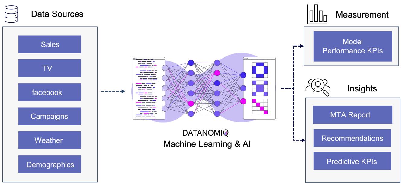
Figure 10 – Attribution Model based on Deep Learning / AI
The approach is scalable, capable of handling large volumes of data, making it ideal for organizations with extensive marketing campaigns and complex customer journeys. By leveraging advanced algorithms, it offers more accurate attribution of credit to different touchpoints, enabling marketers to make informed, data-driven decisions.
All those models are part of the Machine Learning & AI Toolkit for assessing MTA. And since the business world is evolving quickly, newer methods such as double Machine Learning or causal forest models that are discussed in the marketing literature (e.g. Langen & Huber 2023) in combination with eXplainable Artificial Intelligence (XAI) can also be applied as well in the DATANOMIQ Machine Learning and AI framework.
3. Conclusion
As digital marketing continues to evolve in the age of AI, attribution models remain crucial for understanding the complex customer journey and optimizing marketing strategies. These models not only aid in effective budget allocation but also provide a comprehensive view of how different channels contribute to conversions. With advancements in technology, particularly the shift towards data-driven and multi-touch attribution models, marketers are better equipped to make informed decisions that enhance quick return on investment (ROI) and maintain competitiveness in the digital landscape.
Several trends are shaping the evolution of attribution models. The increasing use of machine learning in marketing attribution allows for more precise and predictive analytics, which can anticipate customer behavior and optimize marketing efforts accordingly. Additionally, as privacy regulations become more stringent, there is a growing focus on data quality and ethical data usage (Ethical AI), ensuring that attribution models are both effective and compliant. Furthermore, the integration of view-through attribution, which considers the impact of ad impressions that do not result in immediate clicks, provides a more holistic understanding of customer interactions across channels. As these models become more sophisticated, they will likely incorporate a wider array of data points, offering deeper insights into the customer journey.
Unlock your marketing potential with a strategy session with our DATANOMIQ experts. Discover how our solutions can elevate your media-mix models and boost your organization by making smarter, data-driven decisions.
References
- Zhao, K., Mahboobi, S. H., & Bagheri, S. R. (2018). Shapley value methods for attribution modeling in online advertising. arXiv preprint arXiv:1804.05327.
- Gaur, J., & Bharti, K. (2020). Attribution modelling in marketing: Literature review and research agenda. Academy of Marketing Studies Journal, 24(4), 1-21.
- Langen H, Huber M (2023) How causal machine learning can leverage marketing strategies: Assessing and improving the performance of a coupon campaign. PLoS ONE 18(1): e0278937. https://doi.org/10.1371/journal. pone.0278937
Process Mining – Ist Celonis wirklich so gut? Ein Praxisbericht.
/in Data Engineering, Data Warehousing, Insights, Machine Learning, Main Category, Process Mining, Tool Introduction/by Benjamin AunkoferDiese Artikel wird viel gelesen werden. Von Process Mining Kunden, von Process Mining Beratern und von Process Mining Software-Anbietern. Und ganz besonders von Celonis.
Der Gartner´s Magic Quadrant zu Process Mining Tools für 2024 zeigt einige Movements im Vergleich zu 2023. Jeder kennt den Gartner Magic Quadrant, nicht nur für Process Mining Tools sondern für viele andere Software-Kategorien und auch für Dienstleistungen/Beratungen. Gartner gilt längst als der relevanteste und internationale Benchmark.
Process Mining – Wo stehen wir heute?
Eine Einschränkung dazu vorweg: Ich kann nur für den deutschen Markt sprechen. Zwar verfolge ich mit Spannung die ersten Erfolge von Celonis in den USA und in Japan, aber ich bin dort ja nicht selbst tätig. Ich kann lediglich für den Raum D/A/CH sprechen, in dem ich für Unternehmen in nahezu allen Branchen zu Process Mining Beratung und gemeinsam mit meinem Team Implementierung anbiete. Dabei arbeiten wir technologie-offen und mit nahezu allen Tools – Und oft in enger Verbindung mit Initiativen der Business Intelligence und Data Science. Wir sind neutral und haben keine “Aktien” in irgendeinem Process Mining Tool!
Process Mining wird heute in allen DAX-Konzernen und auch in allen MDAX-Unternehmen eingesetzt. Teilweise noch als Nischenanalytik, teilweise recht großspurig wie es z. B. die Deutsche Telekom oder die Lufthansa tun.
Mittelständische Unternehmen sind hingegen noch wenig erschlossen in Sachen Process Mining, wobei das nicht ganz richtig ist, denn vieles entwickelt sich – so unsere Erfahrung – aus BI / Data Science Projekten heraus dann doch noch in kleinere Process Mining Applikationen, oft ganz unter dem Radar. In Zukunft – da habe ich keinen Zweifel – wird Process Mining jedoch in jedem Unternehmen mit mehr als 1.000 Mitarbeitern ganz selbstverständlich und quasi nebenbei gemacht werden.
Process Mining Software – Was sagt Gartner?
Ich habe mal die Gartner Charts zu Process Mining Tools von 2023 und 2024 übereinandergelegt und erkenne daraus die folgende Entwicklung:
– Celonis bleibt der Spitzenreiter nach Gartner, gerät jedoch zunehmend unter Druck auf dieser Spitzenposition.
– SAP hatte mit dem Kauf von Signavio vermutlich auf das richtige Pferd gesetzt, die Enterprise-Readiness für SAP-Kunden ist leicht erahnbar.
– Die Software AG ist schon lange mit Process Mining am Start, kann sich in ihrer Positionierung nur leicht verbessern.
– Ähnlich wenig Bewegung bei UiPath, in Sachen Completness of Vision immer noch deutlich hinter der Software AG.
– Interessant ist die Entwicklung des deutschen Anbieters MEHRWERK Process Mining (MPM), bei Completness of Vision verschlechtert, bei Ability to Execute verbessert.
– Der deutsche Anbieter process.science, mit MEHRWERK und dem früheren (von Celonis gekauften) PAFnow mindestens vergleichbar, ist hier noch immer nicht aufgeführt.
– Microsoft Process Mining ist der relative Sieger in Sachen Aufholjagd mit ihrer eigenen Lösung (die zum Teil auf dem eingekauften Tool namens Minit basiert). Process Mining wurde kürzlich in die Power Automate Plattform und in Power BI integriert.
– Fluxicon (Disco) ist vom Chart verschwunden. Das ist schade, vom Tool her recht gut mit dem aufgekauften Minit vergleichbar (reine Desktop-Applikation).
Auch wenn ich große Ehrfurcht gegenüber Gartner als Quelle habe, bin ich jedoch nicht sicher, wie weit die Datengrundlage für die Feststellung geht. Ich vertraue soweit der Reputation von Gartner, möchte aber als neutraler Process Mining Experte mit Einblick in den deutschen Markt dazu Stellung beziehen.
Process Mining Tools – Unterschiedliche Erfolgsstories
Aber fangen wir erstmal von vorne an, denn Process Mining Tools haben ihre ganz eigene Geschichte und diese zu kennen, hilft bei der Einordnung von Marktbewegungen etwas und mein Process Mining Software Vergleich auf CIO.de von 2019 ist mittlerweile etwas in die Jahre gekommen. Und Unterhaltungswert haben diese Stories auch, beispielsweise wie ganze Gründer und Teams von diesen Software-Anbietern wie Celonis, UiPath (ehemals ProcessGold), PAFnow (jetzt Celonis), Signavio (jetzt SAP) und Minit (jetzt Microsoft) teilweise im Streit auseinandergingen, eigene Process Mining Tools entwickelt und dann wieder Know How verloren oder selbst aufgekauft wurden – Unter Insidern ist der Gesprächsstoff mit Unterhaltungswert sehr groß.
Dabei darf gerne in Erinnerung gerufen werden, dass Process Mining im Kern eine Graphenanalyse ist, die ein Event Log in Graphen umwandelt, Aktivitäten (Events) stellen dabei die Knoten und die Prozesszeiten die Kanten dar, zumindest ist das grundsätzlich so. Es handelt sich dabei also um eine Analysemethodik und nicht um ein Tool. Ein Process Mining Tool nutzt diese Methodik, stellt im Zweifel aber auch nur exakt diese Visualisierung der Prozessgraphen zur Verfügung oder ein ganzes Tool-Werk von der Datenanbindung und -aufbereitung in ein Event Log bis hin zu weiterführenden Analysen in Richtung des BI-Reportings oder der Data Science.
Im Grunde kann man aber folgende große Herkunftskategorien ausmachen:
1. Process Mining Tools, die als pure Process Mining Software gestartet sind
Hierzu gehört Celonis, das drei-köpfige und sehr geschäftstüchtige Gründer-Team, das ich im Jahr 2012 persönlich kennenlernen durfte. Aber Celonis war nicht das erste Process Mining Unternehmen. Es gab noch einige mehr. Hier fällt mir z. B. das kleine und sympathische Unternehmen Fluxicon ein, dass mit seiner Lösung Disco auch heute noch einen leichtfüßigen Einstieg in Process Mining bietet.
2. Process Mining Tools, die eigentlich aus der Prozessmodellierung oder -automatisierung kommen
Einige Software-Anbieter erkannten frühzeitig (oder zumindest rechtzeitig?), dass Process Mining vielleicht nicht das Kerngeschäft, jedoch eine sinnvolle Ergänzung zu ihrem Portfolio an Software für Prozessmodellierung, -dokumentations oder -automatisierung bietet. Hierzu gehört die Software AG, die eigentlich für ihre ARIS-Prozessmodellierung bekannt war. Und hierzu zählt auch Signavio, die ebenfalls ein reines Prozessmodellierungsprogramm waren und von kurzem von SAP aufgekauft wurden. Aber auch das für RPA bekannte Unternehmen UiPath verleibte sich Process Mining durch den Zukauf von ehemals Process Gold.
3. Process Mining Tools, die Business Intelligence Software erweitern
Und dann gibt es noch diejenigen Anbieter, die bestehende BI Tools mit Erweiterungen zum Process Mining Analysewerkzeug machen. Einer der ersten dieser Anbieter war das Unternehmen PAF (Process Analytics Factory) mit dem Power BI Plugin namens PAFnow, welches von Celonis aufgekauft wurde und heute anscheinend (?) nicht mehr weiterentwickelt wird. Das Unternehmen MEHRWERK, eigentlich ein BI-Dienstleister mit Fokus auf QlikTech-Produkte, bietet für das BI-Tool Qlik Sense ebenfalls eine Erweiterung für Process Mining an und das Unternehmen mit dem unscheinbaren Namen process.science bietet Erweiterungen sowohl für Power BI als auch für Qlik Sense, zukünftig ist eine Erweiterung für Tableu geplant. Process.science fehlt im Gartner Magic Quadrant bis jetzt leider gänzlich, trotz bestehender Marktrelevanz (nach meiner Beobachtung).
Process Mining Tools in der Praxis – Ein Einblick
DAX-Konzerne setzen vor allem auf Celonis. Das Gründer-Team, das starke Vertriebsteam und die Medienpräsenz erst als Unicorn, dann als Decacorn, haben die Türen zu Vorstandsetagen zumindest im mitteleuropäischen Raum geöffnet. Und ganz ehrlich: Dass Celonis ein deutsches Decacorn ist, ist einfach wunderbar. Es ist das erste Decacorn aus Deutschland, das zurzeit wertvollste StartUp in Deutschland und wir können – für den Standort Deutschland – nur hoffen, dass dieser Erfolg bleibt.
Doch wie weit vorne ist Process Mining mit Celonis nun wirklich im Praxiseinsatz? Und ist Celonis für jedes Unternehmen der richtige Einstieg in Process Mining?
Celonis unterscheidet sich von den meisten anderen Tools noch dahingehend, dass es versucht, die ganze Kette des Process Minings in einer einzigen und ausschließlichen Cloud-Anwendung in einer Suite bereitzustellen. Während vor zehn Jahren ich für Celonis noch eine Installation erst einer MS SQL Server Datenbank, etwas später dann bevorzugt eine SAP Hana Datenbank auf einem on-prem Server beim Kunden voraussetzend installieren musste, bevor ich dann zur Installation der Celonis ServerAnwendung selbst kam, ist es heute eine 100% externe Cloud-Lösung. Dies hat anfangs für große Widerstände bei einigen Kunden verursacht, die ehrlicherweise heute jedoch kaum noch eine Rolle spielen. Cloud ist heute selbst für viele mitteleuropäische Unternehmen zum Standard geworden und wird kaum noch infrage gestellt. Vielleicht haben wir auch das ein Stück weit Celonis zu verdanken.
Celonis bietet eine bereits sehr umfassende Anbindung von Datenquellen z. B. für SAP oder Oracle ERP an, mit vordefinierten Event Log SQL Skripten für viele Standard-Prozesse, insbesondere Procure-to-Pay und Order-to-Cash. Aber auch andere Prozesse für andere Geschäftsprozesse z. B. von SalesForce CRM sind bereits verfügbar. Celonis ist zudem der erste Anbieter, der diese Prozessaufbereitung und weiterführende Dashboards in einem App-Store anbietet und so zu einer Plattform wird. Hinzu kommen auch die zuvor als Action Engine bezeichnete Prozessautomation, die mit Lösungen wie Power Automate von Microsoft vergleichbar sind.
Celonis schafft es oftmals in größere Konzerne, ist jedoch selten dann das einzige eingesetzte Process Mining Tool. Meine Kunden und Kontakte aus unterschiedlichsten Unternhemen in Deutschland berichten in Sachen Celonis oft von zu hohen Kosten für die Lizensierung und den Betrieb, zu viel Sales im Vergleich zur Leistung sowie von hohen Aufwänden, wenn der Fokus nicht auf Standardprozesse liegt. Demgegenüber steht jedoch die Tatsache, dass Celonis zumindest für die Standardprozesse bereits viel mitbringt und hier definitiv allen anderen Tool-Anbietern voraus ist und den wohl besten Service bietet.
SAP Signavio rückt nach
Mit dem Aufkauf von Signavio von SAP hat sich SAP meiner Meinung nach an eine gute Position katapultiert. Auch wenn ich vor Jahren noch hätte Wetten können, dass Celonis mal von SAP gekauft wird, scheint der Move mit Signavio nicht schlecht zu wirken, denn ich sehe das Tool bei Kunden mit SAP-Liebe bereits erfolgreich im Einsatz. Dabei scheint SAP nicht den Anspruch zu haben, Signavio zur Plattform für Analytics ausbauen zu wollen, um 1:1 mit Celonis gleichzuziehen, so ist dies ja auch nicht notwendig, wenn Signavio mit SAP Hana und der SAP Datasphere Cloud besser integriert werden wird.
Unternehmen, die am liebsten nur Software von SAP einsetzen, werden also mittlerweile bedient.
Mircosoft holt bei Process Mining auf
Ein absoluter Newcomer unter den Großen Anbietern im praktischen Einsatz bei Unternehmen ist sicherlich Microsoft Process Mining. Ich betreue bereits selbst Kunden, die auf Microsoft setzen und beobachte in meinem Netzwerk ein hohes Interesse an der Lösung von Microsoft. Was als logischer Schritt von Microsoft betrachtet werden kann, ist in der Praxis jedoch noch etwas hakelig, da Microsoft – und ich weiß wovon ich spreche – aktuell noch ein recht komplexes Zusammenspiel aus dem eigentlichen Process Mining Client (ehemals Minit) und der Power Automate Plattform sowie Power BI bereitstellt. Sehr hilfreich ist die Weiterführung der Process Mining Analyse vom Client-Tool dann direkt in der PowerBI Cloud. Das Ganze hat definitiv Potenzial, hängt aber in Details in 2024 noch etwas in diesem Zusammenspiel an verschiedenen Tools, die kein einfaches Setup für den User darstellen.
Doch wenn diese Integration besser funktioniert, und das ist in Kürze zu erwarten, dann bringt das viele Anbieter definitiv in Bedrängnis, denn den Microsoft Stack nutzen die meisten Unternehmen sowieso. Somit wäre kein weiteres Tool für datengetriebene Prozessanalysen mehr notwendig.
Process Mining – Und wie steht es um Machine Learning?
Obwohl ich mich gemeinsam mit Kunden besonders viel mit Machine Learning befasse, sind die Beispiele mit Process Mining noch recht dünn gesäht, dennoch gibt es etwa seit 2020 in Sachen Machine Learning für Process Mining auch etwas zu vermelden.
Celonis versucht Machine Learning innerhalb der Plattform aus einer Hand anzubieten und hat auch eigene Python-Bibleotheken dafür entwickelt. Bisher dreht sich hier viel eher noch um z. B. die Vorhersage von Prozesszeiten oder um die Erkennung von Doppelvorgängen. Die Erkennung von Doppelzahlungen ist sogar eine der penetrantesten Werbeversprechen von Celonis, obwohl eigentlich bereits mit viel einfacherer Analytik effektiv zu bewerkstelligen.
Von Kunden bisher über meinen Geschäftskanal nachgefragte und umgesetzte Machine Learning Funktionen sind u.a. die Anomalie-Erkennung in Prozessdaten, die möglichst frühe Vorhersage von Prozesszeiten (oder -kosten) und die Impact-Prediction auf den Prozess, wenn ein bestimmtes Event eintritt.
Umgesetzt werden diese Anwendungsfälle bisher vor allem auf dritten Plattformen, wie z. B. auf den Analyse-Ressourcen der Microsoft Azure Cloud oder in auf der databricks-Plattform.
Während das nun Anwendungsfälle auf der Prozessanalyse-Seite sind, kann Machine Learning jedoch auf der anderen Seite zur Anwendung kommen: Mit NER-Verfahren (Named Entity Recognition) aus dem NLP-Baukasten (Natural Language Processing) können Event Logs aus unstrukturierten Daten gewonnen werden, z. B. aus Texten in E-Mails oder Tickets.
Data Lakehouse – Event Logs außerhalb des Process Mining Tools
Auch wenn die vorbereitete Anbindung von Standard-ERP-Systemen und deren Standard-Prozesse durch Celonis einen echten Startvorteil bietet, so schwenken Unternehmen immer mehr auf die Etablierung eines unternehmensinternen Data Warehousing oder Data Lakehousing Prozesses, der die Daten als “Data Middlelayer” vorhält und Process Mining Applikationen bereitstellt.
Ich selbst habe diese Beobachtung bereits bei Unternehmen der industriellen Produktion, Handel, Finanzdienstleister und Telekommunikation gemacht und teilweise selbst diese Projekte betreut und/oder umgesetzt. Recht unterschiedlich hingegen ist die interne Benennung dieser Architektur, von “Middlelayer” über “Data Lakehouse” oder “Event Log Layer” bis “Data Hub” waren sehr unterschiedliche Bezeichnungen dabei. Gemeinsam haben sie alle die Funktion als Zwischenebene zwischen den Datenquellen und den Process Mining, BI und Data Science Applikationen.
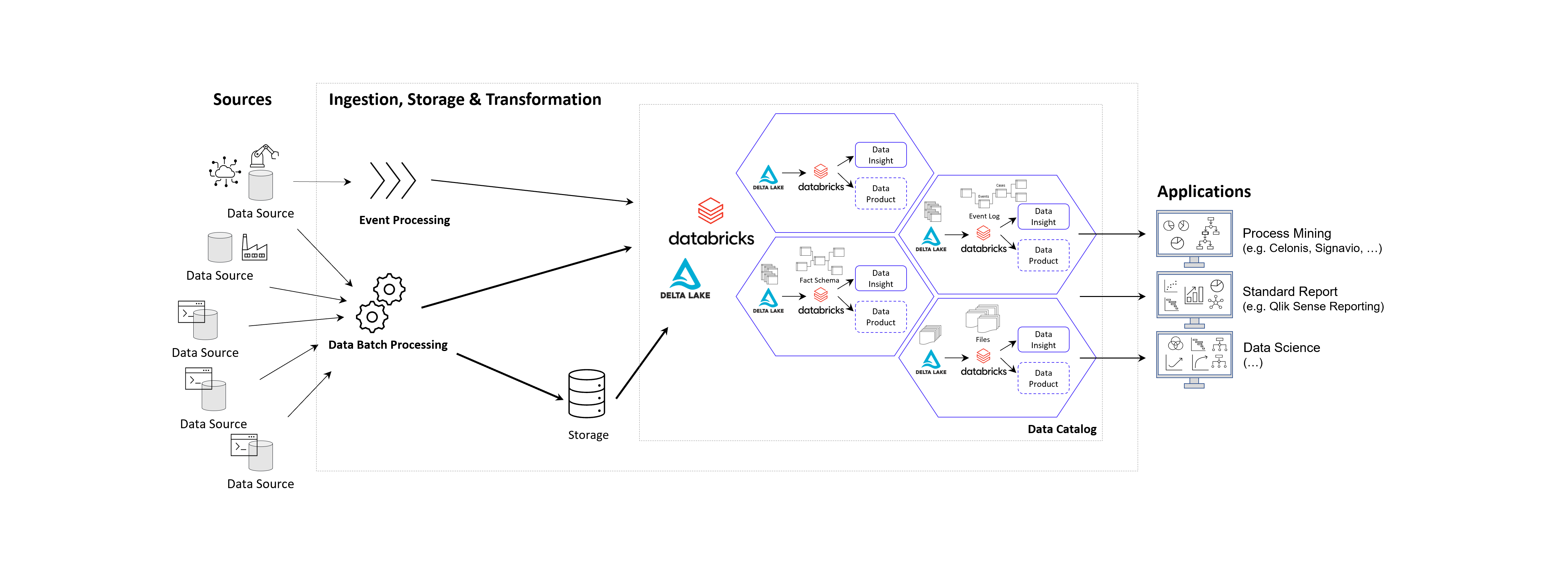
Prinzipielle Architektur-Darstellung eines Data Lakehouse Systems unter Einsatz von Databricks auf der Goolge / Amazon / Microsoft Azure Cloud nach dem Data Mesh Konzept zur Bereitstellung von Data Products für Process Mining, BI und Data Science Applikationen. Alternativ zu Databricks können auch andere Data Warehouse Datenbankplattformen zur Anwendung kommen, beispielsweise auch snowflake mit dbt.
Das Kernziel der Zwischenschicht erstellt für die Process Mining Vohaben die benötigten Event Logs, kann jedoch diesselben Daten für ganz andere Vorhaben und Applikationen zur Verfügung zu stellen.
Vorteile des Data Lakehousing
Die Vorteile einer Daten-Zwischenschicht in Form eines Data Warehouses oder Data Lakehouses sind – je nach unternehmensinterner Ausrichtung – beispielsweise die folgenden:
- Keine doppelte Datenhaltung, denn Daten können zentral gehalten werden und in Views speziellen Applikationen der BI, Data Science, KI und natürlich auch für Process Mining genutzt werden.
- Einfachere Data Governance, denn eine zentrale Datenschicht zwischen den Applikationen erleichtert die Übersicht und die Aussteuerung der Datenzugriffsberechtigung.
- Reduzierte Cloud Kosten, denn Cloud Tools berechnen Gebühren für die Speicherung von Daten. Müssen Rohdatentabellen in die Analyse-Tools wie z. B. Celonis geladen werden, kann dies unnötig hohe Kosten verursachen.
- Reduzierte Personalkosten, sind oft dann gegeben, wenn interne Data Engineers verfügbar sind, die die Datenmodelle intern entwickeln.
- Höhere Data Readiness, denn für eine zentrale Datenplattform lohn es sich eher, Daten aus weniger genutzten Quellen anzuschließen. Hier ergeben sich oft neue Chancen der Datenfusion für nützliche Analysen, die vorher nicht angedacht waren, weil sich der Aufwand nur hierfür speziell nicht lohne.
- Große Datenmodelle werden möglich und das Investment in diese lohnt sich nun, da sie für verschiedene Process Mining Tools ausgeliefert werden können, oder auch nur Sichten (Views) auf Prozess-Perspektiven. So wird Object-centric Process Mining annäherend mit jedem Tool möglich.
- Nutzung von heterogenen Datenquellen, denn mit einem Data Lakehouse ist auch die Nutzung von unstrukturierten Daten leicht möglich, davon wird in Zukunft auch Process Mining profitieren. Denn dank KI und NLP (Data Science) können auch Event Logs aus unstrukturierten Daten generiert werden.
- Unabhängigkeit von Tool-Anbietern, denn wenn die zentrale Datenschicht die Daten in Datenmodelle aufbereitet (im Falle von Process Mining oft in normalisierten Event Logs), können diese allen Tools zur Verfügung gestellt werden. Dies sorgt für Unabhängigkeit gegenüber einzelnen Tool-Anbietern.
- Data Science und KI wird erleichtert, denn die Data Science und das Training im Machine Learning kann direkt mit dem reichhaltigen Pool an Daten erfolgen, auch direkt mit den Daten der Event Logs und losgelöst vom Process Mining Analyse-Tool, z. B. in Databricks oder den KI-Tools von Google, AWS und Mircosoft Azure (Azure Cognitive Services, Azure Machine Learning etc.).
Unter diesen Aspekten wird die Tool-Auswahl für die Prozessanalyse selbst in ihrer Relevanz abgemildert, da diese Tools schneller ausgetauscht werden können. Dies könnte auch bedeuten, dass sich für Unternehmen die Lösung von Microsoft besonders anbietet, da das Data Engineering und die Data Science sowieso über andere Cloud Services abgebildet wird, jedoch kein weiterer Tool-Anbieter eingebunden werden muss.
Process Mining Software – Fazit
Es ist viel Bewegung am Markt und bietet dem Beobachter auch tatsächlich etwas Entertainment. Celonis ist weiterhin der Platzhirsch und wir können sehr froh sein, dass wir es hier mit einem deutschen Start-Up zutun haben. Für Unternehmen, die gleich voll in Process Mining reinsteigen möchten und keine Scheu vor einem möglichen Vendor-Lock-In, bietet Celonis meiner Ansicht nach immer noch das beste Angebot, wenn auch nicht die günstigste Lösung. Die anderen Tools können ebenfalls eine passende Lösung sein, nicht nur aus preislichen Gründen, sondern vor allem im Kontext der zu untersuchenden Prozesse, der Datenquellen und der bestehenden Tool-Landschaft. Dies sollte im Einzelfall geprüft werden.
Die Datenbereitstellung und -aufbereitung sollte idealerweise nicht im Process Mining Tool erfolgen, sondern auf einer zentralen Datenschicht als Data Warehouse oder Data Lakehouse für Process Mining. Die damit gewonnene Data Readiness zahlt nicht nur auf datengetriebene Prozessanalysen ein, sondern kommt dem ganzen Unternehmen zu Gute und ermöglicht zukünftige Projekte mit Daten, an die vorher oder bisher gar nicht zu denken waren.
Dieser Artikel wurde von Benjamin Aunkofer, einem neutralen Process Mining Berater, ohne KI (ohne ChatGPT etc.) verfasst!
KI in der Abschlussprüfung – Podcast mit Benjamin Aunkofer
/in Artificial Intelligence, Big Data, Data Science, Insights, Interviews, Machine Learning, Reinforcement Learning/by AUDAVISGemeinsam mit Prof. Kai-Uwe Marten von der Universität Ulm und dortiger Direktor des Instituts für Rechnungswesen und Wirtschaftsprüfung, bespricht Benjamin Aunkofer, Co-Founder und Chief AI Officer von AUDAVIS, die Potenziale und heutigen Möglichkeiten von der Künstlichen Intelligenz (KI) in der Jahresabschlussprüfung bzw. allgemein in der Wirtschaftsprüfung: KI als Co-Pilot für den Abschlussprüfer.
Inhaltlich behandelt werden u.a. die Möglichkeiten von überwachtem und unüberwachten maschinellem Lernen, die Möglichkeit von verteiltem KI-Training auf Datensätzen sowie warum Large Language Model (LLM) nur für einige bestimmte Anwendungsfälle eine adäquate Lösung darstellen.
Die neue Folge ist frei verfügbar zum visuellen Ansehen oder auch nur zum Anhören, bitte besuchen Sie dafür einen der folgenden Links:
… Spotify: Podcast “Wirtschaftsprüfung kann mehr” auf Spotify
… YouTube: Ulmer Forum für Wirtschaftswissenschaften auf Youtube
… und auf der Podcast-Webseite unter Podcast – Wirtschaftsprüfung kann mehr!
Object-centric Process Mining on Data Mesh Architectures
/in Artificial Intelligence, Big Data, Business Analytics, Business Intelligence, Cloud, Data Engineering, Data Mining, Data Science, Data Warehousing, Industrie 4.0, Machine Learning, Main Category, Predictive Analytics, Process Mining/by Benjamin AunkoferIn addition to Business Intelligence (BI), Process Mining is no longer a new phenomenon, but almost all larger companies are conducting this data-driven process analysis in their organization.
The database for Process Mining is also establishing itself as an important hub for Data Science and AI applications, as process traces are very granular and informative about what is really going on in the business processes.
The trend towards powerful in-house cloud platforms for data and analysis ensures that large volumes of data can increasingly be stored and used flexibly. This aspect can be applied well to Process Mining, hand in hand with BI and AI.
New big data architectures and, above all, data sharing concepts such as Data Mesh are ideal for creating a common database for many data products and applications.
The Event Log Data Model for Process Mining
Process Mining as an analytical system can very well be imagined as an iceberg. The tip of the iceberg, which is visible above the surface of the water, is the actual visual process analysis. In essence, a graph analysis that displays the process flow as a flow chart. This is where the processes are filtered and analyzed.
The lower part of the iceberg is barely visible to the normal analyst on the tool interface, but is essential for implementation and success: this is the Event Log as the data basis for graph and data analysis in Process Mining. The creation of this data model requires the data connection to the source system (e.g. SAP ERP), the extraction of the data and, above all, the data modeling for the event log.
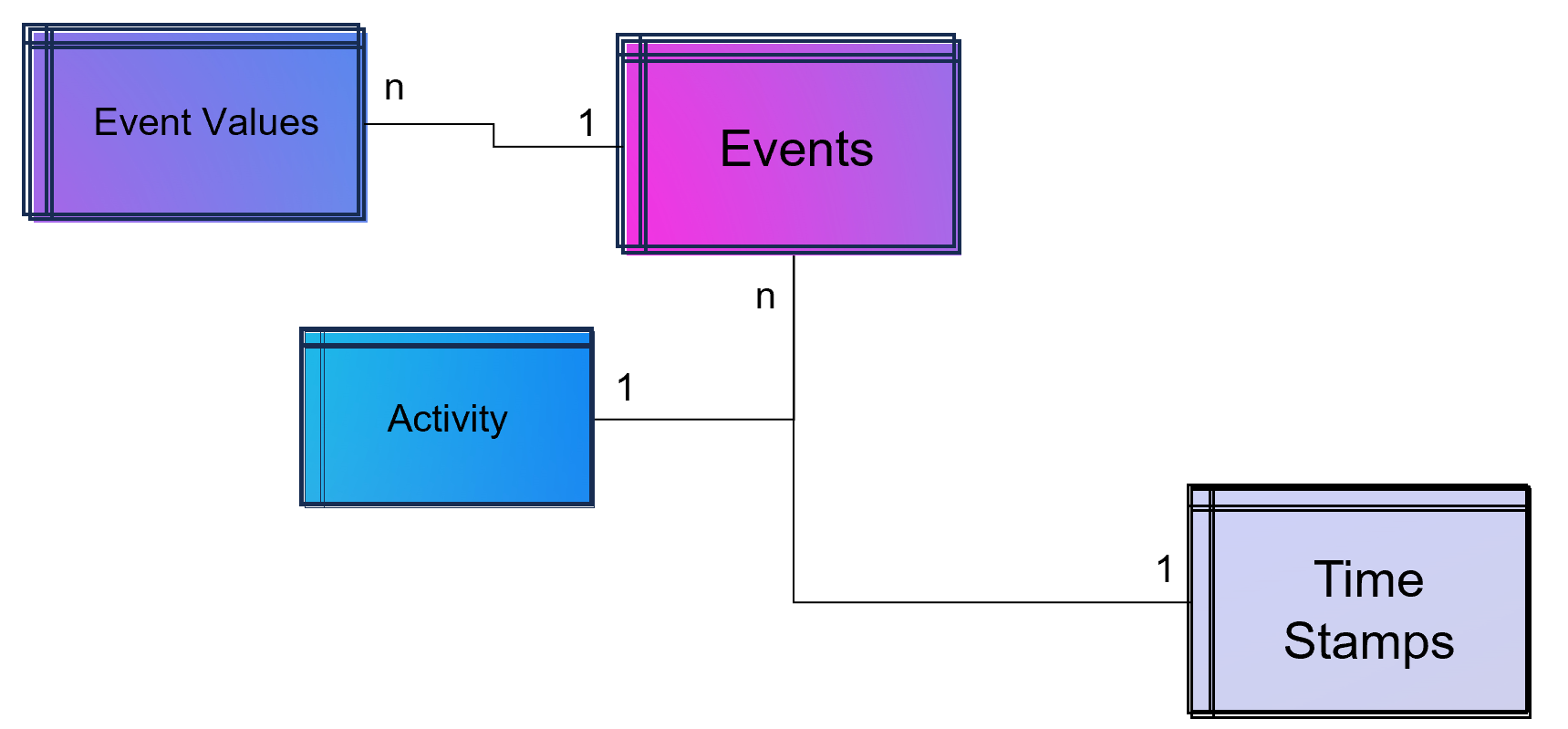
Simple Data Model for a Process Mining Event Log.
As part of data engineering, the data traces that indicate process activities are brought into a log-like schema. A simple event log is therefore a simple table with the minimum requirement of a process number (case ID), a time stamp and an activity description.
An Event Log can be seen as one big data table containing all the process information. Splitting this big table into several data tables is due to the goal of increasing the efficiency of storing the data in a normalized database.
The following example SQL-query is inserting Event-Activities from a SAP ERP System into an existing event log database table (one big table). It shows that events are based on timestamps (CPUDT, CPUTM) and refer each to one of a list of possible activities (dependent on VGABE).
|
1 2 3 4 5 6 7 8 9 10 11 12 13 14 15 16 17 18 19 20 21 22 23 24 25 26 27 28 29 30 31 32 33 34 35 36 37 |
/* Inserting Events of Material Movement of Purchasing Processes */ INSERT INTO Event_Log SELECT EKBE.EBELN AS Einkaufsbeleg ,EKBE.EBELN + EKBE.EBELP AS PurchaseOrderPosition-- <-- Case ID of this Purchasing Process ,MSEG_MKPF.AUFNR AS CustomerOrder ,NULL AS CustomerOrderPosition ,CASE -- <-- Activitiy Description dependent on a flag WHEN MSEG_MKPF.VGABE = 'WA' THEN 'Warehouse Outbound for Customer Order' WHEN MSEG_MKPF.VGABE = 'WF' THEN 'Warehouse Inbound for Customer Order' WHEN MSEG_MKPF.VGABE = 'WO' THEN 'Material Movement for Manufacturing' WHEN MSEG_MKPF.VGABE = 'WE' THEN 'Warehouse Inbound for Purchase Order' WHEN MSEG_MKPF.VGABE = 'WQ' THEN 'Material Movement for Stock' WHEN MSEG_MKPF.VGABE = 'WR' THEN 'Material Movement after Manufacturing' ELSE 'Material Movement (other)' END AS Activity ,EKPO.MATNR AS Material -- <-- ,NULL AS StorageType ,MSEG_MKPF.LGORT AS StorageLocation ,SUBSTRING(MSEG_MKPF.CPUDT ,1,2) + '-' + SUBSTRING(MSEG_MKPF.CPUDT,4,2) + '-' + SUBSTRING(MSEG_MKPF.CPUDT,7,4) + ' ' + SUBSTRING(MSEG_MKPF.CPUTM,1,8) + '.0000' AS EventTime ,'020' AS Sorting ,MSEG_MKPF.USNAM AS EventUser ,EKBE.MATNR AS Material ,MSEG_MKPF.BWART AS MovementType ,MSEG_MKPF.MANDT AS Mandant FROM SAP.EKBE LEFT JOIN SAP.EKPO ON EKBE.MANDT = EKPO.MANDT AND EKBE.BUKRS = EKPO.BURKSEKBE.EBELN = EKPO.EBELN AND EKBE.Pos = EKPO.Pos LEFT JOIN SAP.MSEG_MKPF AS MSEG_MKPF -- <-- Here as a pre-join of MKPF & MSEG table ON EKBE.MANDT = MSEG_MKPF.MANDT AND EKBE.BURKS = MSEG.BUKRSMSEG_MKPF.MATNR = EKBE.MATNR AND MSEG_MKPF.EBELP = EKBE.EBELP WHERE EKBE.VGABE= '1' -- <-- OR EKBE.VGABE= '2' -- Warehouse Outbound -> VGABE = 1, Invoice Inbound -> VGABE = 2 |
Attention: Please see this SQL as a pure example of event mining for a classic (single table) event log! It is based on a German SAP ERP configuration with customized processes.
An Event Log can also include many other columns (attributes) that describe the respective process activity in more detail or the higher-level process context.
Incidentally, Process Mining can also work with more than just one timestamp per activity. Even the small Process Mining tool Fluxicon Disco made it possible to handle two activities from the outset. For example, when creating an order in the ERP system, the opening and closing of an input screen could be recorded as a timestamp and the execution time of the micro-task analyzed. This concept is continued as so-called task mining.
Task Mining
Task Mining is a subtype of Process Mining and can utilize user interaction data, which includes keystrokes, mouse clicks or data input on a computer. It can also include user recordings and screenshots with different timestamp intervals.
As Task Mining provides a clearer insight into specific sub-processes, program managers and HR managers can also understand which parts of the process can be automated through tools such as RPA. So whenever you hear that Process Mining can prepare RPA definitions you can expect that Task Mining is the real deal.
Machine Learning for Process and Task Mining on Text and Video Data
Process Mining and Task Mining is already benefiting a lot from Text Recognition (Named-Entity Recognition, NER) by Natural Lamguage Processing (NLP) by identifying events of processes e.g. in text of tickets or e-mails. And even more Task Mining will benefit form Computer Vision since videos of manufacturing processes or traffic situations can be read out. Even MTM analysis can be done with Computer Vision which detects movement and actions in video material.
Object-Centric Process Mining
Object-centric Process Data Modeling is an advanced approach of dynamic data modelling for analyzing complex business processes, especially those involving multiple interconnected entities. Unlike classical process mining, which focuses on linear sequences of activities of a specific process chain, object-centric process mining delves into the intricacies of how different entities, such as orders, items, and invoices, interact with each other. This method is particularly effective in capturing the complexities and many-to-many relationships inherent in modern business processes.
Note from the author: The concept and name of object-centric process mining was introduced by Wil M.P. van der Aalst 2019 and as a product feature term by Celonis in 2022 and is used extensively in marketing. This concept is based on dynamic data modelling. I probably developed my first event log made of dynamic data models back in 2016 and used it for an industrial customer. At that time, I couldn’t use the Celonis tool for this because you could only model very dedicated event logs for Celonis and the tool couldn’t remap the attributes of the event log while on the other hand a tool like Fluxicon disco could easily handle all kinds of attributes in an event log and allowed switching the event perspective e.g. from sales order number to material number or production order number easily.
An object-centric data model is a big deal because it offers the opportunity for a holistic approach and as a database a single source of truth for Process Mining but also for other types of analytical applications.
Enhancement of the Data Model for Obect-Centricity
The Event Log is a data model that stores events and their related attributes. A classic Event Log has next to the Case ID, the timestamp and a activity description also process related attributes containing information e.g. about material, department, user, amounts, units, prices, currencies, volume, volume classes and much much more. This is something we can literally objectify!
The problem of this classic event log approach is that this information is transformed and joined to the Event Log specific to the process it is designed for.
An object-centric event log is a central data store for all kind of events mapped to all relevant objects to these events. For that reason our event log – that brings object into the center of gravity – we need a relational bridge table (Event_Object_Relation) into the focus. This tables creates the n to m relation between events (with their timestamps and other event-specific values) and all objects.
For fulfillment of relational database normalization the object table contains the object attributes only but relates their object attribut values from another table to these objects.
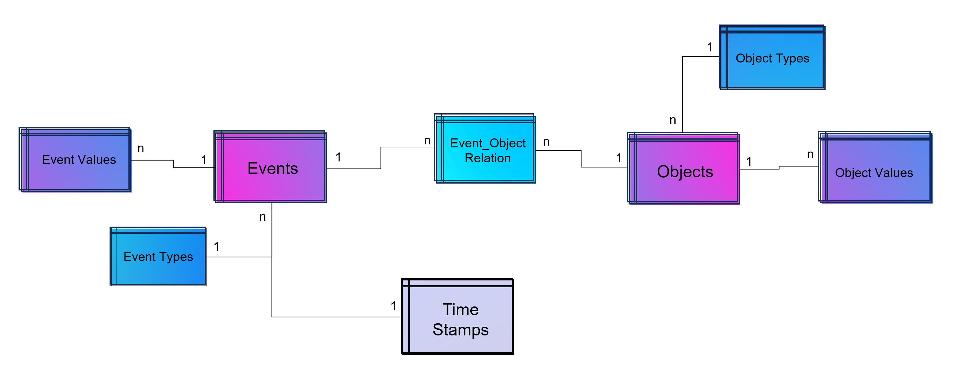
Advanced Event Log with dynamic Relations between Objects and Events
The above showed data model is already object-centric but still can become more dynamic in order to object attributes by object type (e.g. the type material will have different attributes then the type invoice or department). Furthermore the problem that not just events and their activities have timestamps but also objects can have specific timestamps (e.g. deadline or resignation dates).
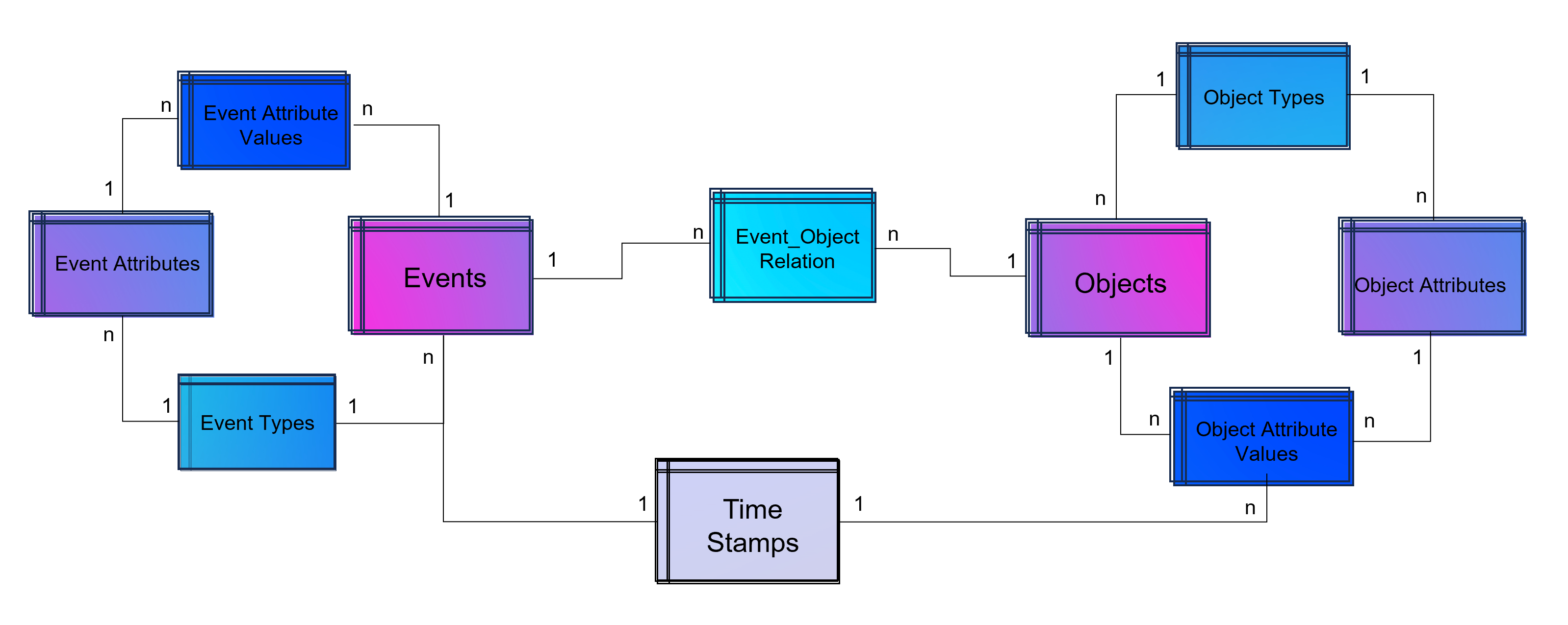
Advanced Event Log with dynamic Relations between Objects and Events and dynamic bounded attributes and their values to Events – And the same for Objects.
A last step makes the event log data model more easy to analyze with BI tools: Adding a classical time dimension adding information about each timestamp (by date, not by time of day), e.g. weekdays or public holidays.
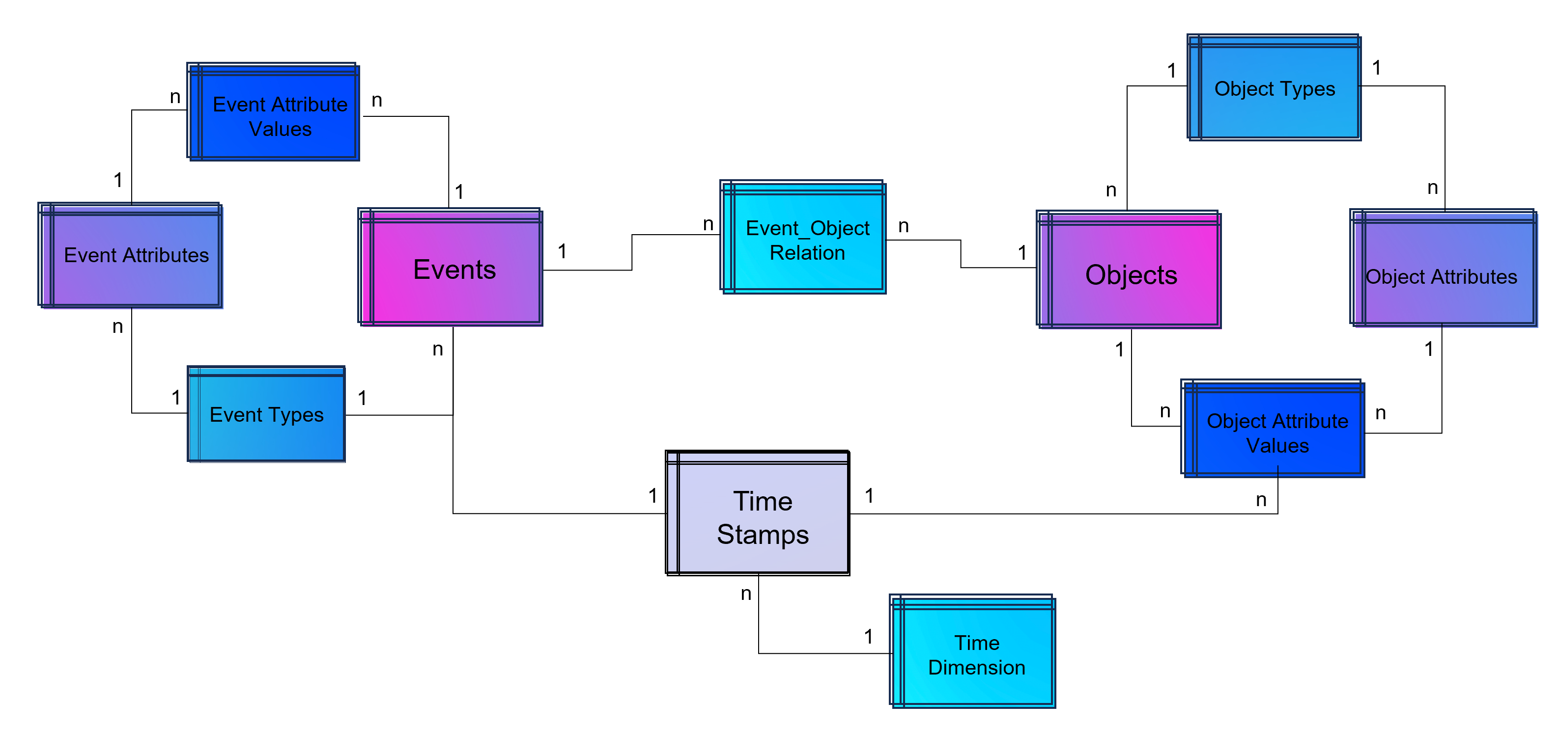
Advanced Event Log with dynamic Relations between Objects and Events and dynamic bounded attributes and their values to Events and Objects. The measured timestamps (and duration times in case of Task Mining) are enhanced with a time-dimension for BI applications.
For analysis the way of Business Intelligence this normalized data model can already be used. On the other hand it is also possible to transform it into a fact-dimensional data model like the star schema (Kimball approach). Also Data Science related use cases will find granular data e.g. for training a regression model for predicting duration times by process.
Note from the author: Process Mining is often regarded as a separate discipline of analysis and this is a justified classification, as process mining is essentially a graph analysis based on the event log. Nevertheless, process mining can be considered a sub-discipline of business intelligence. It is therefore hardly surprising that some process mining tools are actually just a plugin for Power BI, Tableau or Qlik.
Storing the Object-Centrc Analytical Data Model on Data Mesh Architecture
Central data models, particularly when used in a Data Mesh in the Enterprise Cloud, are highly beneficial for Process Mining, Business Intelligence, Data Science, and AI Training. They offer consistency and standardization across data structures, improving data accuracy and integrity. This centralized approach streamlines data governance and management, enhancing efficiency. The scalability and flexibility provided by data mesh architectures on the cloud are very beneficial for handling large datasets useful for all analytical applications.
Note from the author: Process Mining data models are very similar to normalized data models for BI reporting according to Bill Inmon (as a counterpart to Ralph Kimball), but are much more granular. While classic BI is satisfied with the header and item data of orders, process mining also requires all changes to these orders. Process mining therefore exceeds this data requirement. Furthermore, process mining is complementary to data science, for example the prediction of process runtimes or failures. It is therefore all the more important that these efforts in this treasure trove of data are centrally available to the company.
Central single source of truth models also foster collaboration, providing a common data language for cross-functional teams and reducing redundancy, leading to cost savings. They enable quicker data processing and decision-making, support advanced analytics and AI with standardized data formats, and are adaptable to changing business needs.
Central data models in a cloud-based Data Mesh Architecture (e.g. on Microsoft Azure, AWS, Google Cloud Platform or SAP Dataverse) significantly improve data utilization and drive effective business outcomes. And that´s why you should host any object-centric data model not in a dedicated tool for analysis but centralized on a Data Lakehouse System.
About the Process Mining Tool for Object-Centric Process Mining
Celonis is the first tool that can handle object-centric dynamic process mining event logs natively in the event collection. However, it is not neccessary to have Celonis for using object-centric process mining if you have the dynamic data model on your own cloud distributed with the concept of a data mesh. Other tools for process mining such as Signavio, UiPath, and process.science or even the simple desktop tool Fluxicon Disco can be used as well. The important point is that the data mesh approach allows you to easily generate classic event logs for each analysis perspective using the dynamic object-centric data model which can be used for all tools of process visualization…
… and you can also use this central data model to generate data extracts for all other data applications (BI, Data Science, and AI training) as well!
Data Mesh Architecture on Cloud for BI, Data Science and Process Mining
/in Artificial Intelligence, Big Data, Business Analytics, Business Intelligence, Cloud, Data Engineering, Data Science, Machine Learning, Main Category, Predictive Analytics, Process Mining, Tool Introduction, Use Cases/by Benjamin AunkoferCompanies use Business Intelligence (BI), Data Science, and Process Mining to leverage data for better decision-making, improve operational efficiency, and gain a competitive edge. BI provides real-time data analysis and performance monitoring, while Data Science enables a deep dive into dependencies in data with data mining and automates decision making with predictive analytics and personalized customer experiences. Process Mining offers process transparency, compliance insights, and process optimization. The integration of these technologies helps companies harness data for growth and efficiency.
Applications of BI, Data Science and Process Mining grow together
More and more all these disciplines are growing together as they need to be combined in order to get the best insights. So while Process Mining can be seen as a subpart of BI while both are using Machine Learning for better analytical results. Furthermore all theses analytical methods need more or less the same data sources and even the same datasets again and again.
Bring separate(d) applications together with Data Mesh
While all these analytical concepts grow together, they are often still seen as separated applications. There often remains the question of responsibility in a big organization. If this responsibility is decided as not being a central one, Data Mesh could be a solution.
Data Mesh is an architectural approach for managing data within organizations. It advocates decentralizing data ownership to domain-oriented teams. Each team becomes responsible for its Data Products, and a self-serve data infrastructure is established. This enables scalability, agility, and improved data quality while promoting data democratization.
In the context of a Data Mesh, a Data Product refers to a valuable dataset or data service that is managed and owned by a specific domain-oriented team within an organization. It is one of the key concepts in the Data Mesh architecture, where data ownership and responsibility are distributed across domain teams rather than centralized in a single data team.
A Data Product can take various forms, depending on the domain’s requirements and the data it manages. It could be a curated dataset, a machine learning model, an API that exposes data, a real-time data stream, a data visualization dashboard, or any other data-related asset that provides value to the organization.
However, successful implementation requires addressing cultural, governance, and technological aspects. One of this aspect is the cloud architecture for the realization of Data Mesh.
Example of a Data Mesh on Microsoft Azure Cloud using Databricks
The following image shows an example of a Data Mesh created and managed by DATANOMIQ for an organization which uses and re-uses datasets from various data sources (ERP, CRM, DMS, IoT,..) in order to provide the data as well as suitable data models as data products to applications of Data Science, Process Mining (Celonis, UiPath, Signavio & more) and Business Intelligence (Tableau, Power BI, Qlik & more).
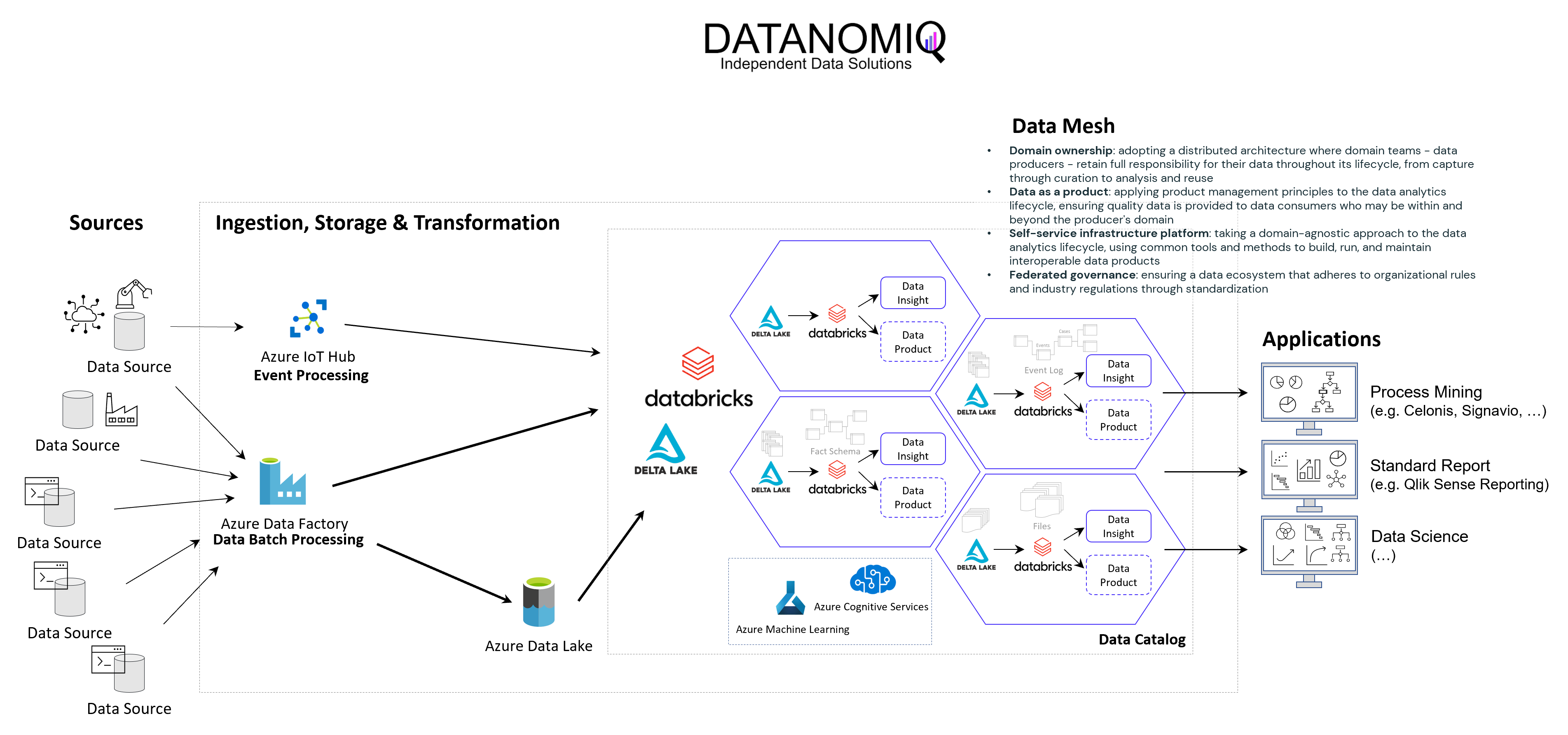
Data Mesh on Azure Cloud with Databricks and Delta Lake for Applications of Business Intelligence, Data Science and Process Mining.
Microsoft Azure Cloud is favored by many companies, especially for European industrial companies, due to its scalability, flexibility, and industry-specific solutions. It offers robust IoT and edge computing capabilities, advanced data analytics, and AI services. Azure’s strong focus on security, compliance, and global presence, along with hybrid cloud capabilities and cost management tools, make it an ideal choice for industrial firms seeking to modernize, innovate, and improve efficiency. However, this concept on the Azure Cloud is just an example and can easily be implemented on the Google Cloud (GCP), Amazon Cloud (AWS) and now even on the SAP Cloud (Datasphere) using Databricks.
Databricks is an ideal tool for realizing a Data Mesh due to its unified data platform, scalability, and performance. It enables data collaboration and sharing, supports Delta Lake for data quality, and ensures robust data governance and security. With real-time analytics, machine learning integration, and data visualization capabilities, Databricks facilitates the implementation of a decentralized, domain-oriented data architecture we need for Data Mesh.
Furthermore there are also alternate architectures without Databricks but more cloud-specific resources possible, for Microsoft Azure e.g. using Azure Synapse instead. See this as an example which has many possible alternatives.
Summary – What value can you expect?
With the concept of Data Mesh you will be able to access all your organizational internal and external data sources once and provides the data as several data models for all your analytical applications. The data models are seen as data products with defined value, costs and ownership. Each applications has its own data model. While Data Science Applications have more raw data, BI applications get their well prepared star schema galaxy models, and Process Mining apps get normalized event logs. Using data sharing (in Databricks: Delta Sharing) data products or single datasets can be shared through applications and owners.
Monitoring of Jobskills with Data Engineering & AI
/in Artificial Intelligence, Business Intelligence, Carrier, Data Engineering, Data Mining, Data Science, Deep Learning, Gerneral, Insights, Machine Learning, Main Category, Natural Language Processing, Visualization/by Benjamin AunkoferOn own account, we from DATANOMIQ have created a web application that monitors data about job postings related to Data & AI from multiple sources (Indeed.com, Google Jobs, Stepstone.de and more).
The data is obtained from the Internet via APIs and web scraping, and the job titles and the skills listed in them are identified and extracted from them using Natural Language Processing (NLP) or more specific from Named-Entity Recognition (NER).
The skill clusters are formed via the discipline of Topic Modelling, a method from unsupervised machine learning, which show the differences in the distribution of requirements between them.
The whole web app is hosted and deployed on the Microsoft Azure Cloud via CI/CD and Infrastructure as Code (IaC).
The presentation is currently limited to the current situation on the labor market. However, we collect these over time and will make trends secure, for example how the demand for Python, SQL or specific tools such as dbt or Power BI changes.
Why we did it? It is a nice show-case many people are interested in. Over the time, it will provides you the answer on your questions related to which tool to learn! For DATANOMIQ this is a show-case of the coming Data as a Service (DaaS) Business.
Was ist eine Vektor-Datenbank? Und warum spielt sie für AI eine so große Rolle?
/in Artificial Intelligence, Big Data, Business Analytics, Data Mining, Insights, Machine Learning, Natural Language Processing, Predictive Analytics, Use Cases/by Benjamin AunkoferWie können Unternehmen und andere Organisationen sicherstellen, dass kein Wissen verloren geht? Intranet, ERP, CRM, DMS oder letztendlich einfach Datenbanken mögen die erste Antwort darauf sein. Doch Datenbanken sind nicht gleich Datenbanken, ganz besonders, da operative IT-Systeme meistens auf relationalen Datenbanken aufsetzen. In diesen geht nur leider dann doch irgendwann das Wissen verloren… Und das auch dann, wenn es nie aus ihnen herausgelöscht wird!
Die meisten Datenbanken sind darauf ausgelegt, Daten zu speichern und wieder abrufbar zu machen. Neben den relationalen Datenbanken (SQL) gibt es auch die NoSQL-Datenbanken wie den Key-Value-Store, Dokumenten- und Graph-Datenbanken mit recht speziellen Anwendungsgebieten. Vektor-Datenbanken sind ein weiterer Typ von Datenbank, die unter Einsatz von AI (Deep Learning, n-grams, …) Wissen in Vektoren übersetzen und damit vergleichbarer und wieder auffindbarer machen. Diese Funktion der Datenbank spielt seinen Vorteil insbesondere bei vielen Dimensionen aus, wie sie Text- und Bild-Daten haben.
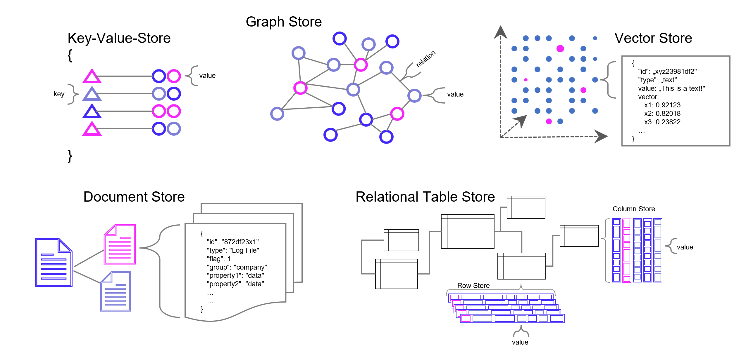
Datenbank-Typen in grobkörniger Darstellung. Es gibt in der Realität jedoch viele Feinheiten, Übergänge und Überbrückungen zwischen den Datenbanktypen, z. B. zwischen emulierter und nativer Graph-Datenbank. Manche Dokumenten- Vektor-Datenbanken können auch relationale Datenmodellierung. Und eigentlich relationale Datenbanken wie z. B. PostgreSQL können mit Zusatzmodulen auch Vektoren verarbeiten.
Vektor-Datenbanken speichern Daten grundsätzlich nicht relational oder in einer anderen Form menschlich konstruierter Verbindungen. Dennoch sichert die Datenbank gewissermaßen Verbindungen indirekt, die von Menschen jedoch – in einem hochdimensionalen Raum – nicht mehr hergeleitet werden können und sich auf bestimmte Kontexte beziehen, die sich aus den Daten selbst ergeben. Maschinelles Lernen kommt mit der nummerischen Auflösung von Text- und Bild-Daten (und natürlich auch bei ganz anderen Daten, z. B. Sound) am besten zurecht und genau dafür sind Vektor-Datenbanken unschlagbar.
Was ist eine Vektor-Datenbank?
Eine Vektordatenbank speichert Vektoren neben den traditionellen Datenformaten (Annotation) ab. Ein Vektor ist eine mathematische Struktur, ein Element in einem Vektorraum, der eine Reihe von Dimensionen hat (oder zumindest dann interessant wird, genaugenommen starten wir beim Null-Vektor). Jede Dimension in einem Vektor repräsentiert eine Art von Information oder Merkmal. Ein gutes Beispiel ist ein Vektor, der ein Bild repräsentiert: jede Dimension könnte die Intensität eines bestimmten Pixels in dem Bild repräsentieren.
Auf diese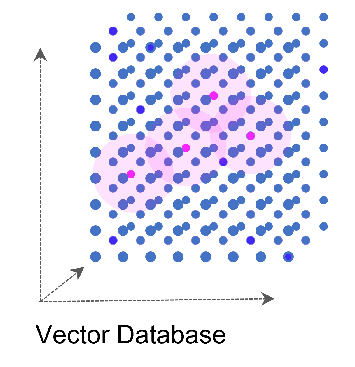 Weise kann eine ganze Sammlung von Bildern als eine Sammlung von Vektoren dargestellt werden. Noch gängiger jedoch sind Vektorräume, die Texte z. B. über die Häufigkeit des Auftretens von Textbausteinen (Wörter, Silben, Buchstaben) in sich einbetten (Embeddings). Embeddings sind folglich Vektoren, die durch die Projektion des Textes auf einen Vektorraum entstehen.
Vektor-Datenbanken sind besonders nützlich, wenn man Ähnlichkeiten zwischen Vektoren finden muss, z. B. ähnliche Bilder in einer Sammlung oder die Wörter “Hund” und “Katze”, die zwar in ihren Buchstaben keine Ähnlichkeit haben, jedoch in ihrem Kontext als Haustiere. Mit Vektor-Algorithmen können diese Ähnlichkeiten schnell und effizient aufgespürt werden, was sich mit traditionellen relationalen Datenbanken sehr viel schwieriger und vor allem ineffizienter darstellt.
Vektordatenbanken können auch hochdimensionale Daten effizient verarbeiten, was in vielen modernen Anwendungen, wie zum Beispiel Deep Learning, wichtig ist. Einige Beispiele für Vektordatenbanken sind Elasticsearch / Vector Search, Weaviate, Faiss von Facebook und Annoy von Spotify.
Viele Lernalgorithmen des maschinellen Lernens basieren auf Vektor-basierter Ähnlichkeitsmessung, z. B. der k-Nächste-Nachbarn-Prädiktionsalgorithmus (Regression/Klassifikation) oder K-Means-Clustering. Die Ähnlichkeitsbetrachtung erfolgt mit Distanzmessung im Vektorraum. Die dafür bekannteste Methode, die Euklidische Distanz zwischen zwei Punkten, basiert auf dem Satz des Pythagoras (Hypotenuse ist gleich der Quadratwurzel aus den beiden Dimensions-Katheten im Quadrat, im zwei-dimensionalen Raum). Es kann jedoch sinnvoll sein, aus Gründen der Effizienz oder besserer Konvergenz des maschinellen Lernens andere als die Euklidische Distanz in Betracht zu ziehen.
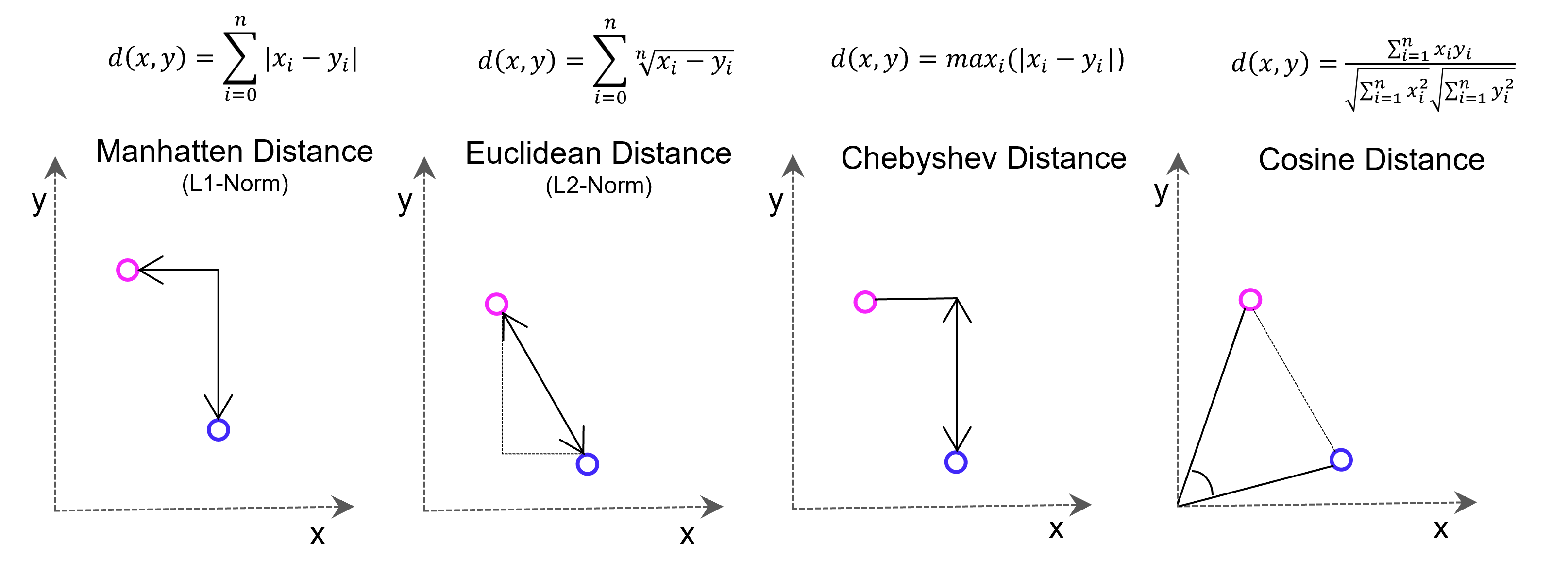
Vectore-based distance measuring methods: Euclidean Distance L2-Norm, Manhatten Distance L1-Norm, Chebyshev Distance and Cosine Distance
Vektor-Datenbanken für Deep Learning
Der Aufbau von künstlichen Neuronalen Netzen im Deep Learning sieht nicht vor, dass ganze Sätze in ihren textlichen Bestandteilen in das jeweilige Netz eingelesen werden, denn sie funktionieren am besten mit rein nummerischen Input. Die Texte müssen in diese transformiert werden, eventuell auch nach diesen in Cluster eingeteilt und für verschiedene Trainingsszenarien separiert werden.
Vektordatenbanken werden für die Datenvorbereitung (Annotation) und als Trainingsdatenbank für Deep Learning zur effizienten Speicherung, Organisation und Manipulation der Texte genutzt. Für Natural Language Processing (NLP) benötigen Modelle des Deep Learnings die zuvor genannten Word Embedding, also hochdimensionale Vektoren, die Informationen über Worte, Sätze oder Dokumente repräsentieren. Nur eine Vektordatenbank macht diese effizient abrufbar.
Vektor-Datenbank und Large Language Modells (LLM)
Ohne Vektor-Datenbanken wären die Erfolge von OpenAI und anderen Anbietern von LLMs nicht möglich geworden. Aber fernab der Entwicklung in San Francisco kann jedes Unternehmen unter Einsatz von Vektor-Datenbanken und den APIs von Google, OpenAI / Microsoft oder mit echten Open Source LLMs (Self-Hosting) ein wahres Orakel über die eigenen Unternehmensdaten herstellen. Dazu werden über APIs die Embedding-Engines z. B. von OpenAI genutzt. Wir von DATANOMIQ nutzen diese Architektur, um Unternehmen und andere Organisationen dazu zu befähigen, dass kein Wissen mehr verloren geht.
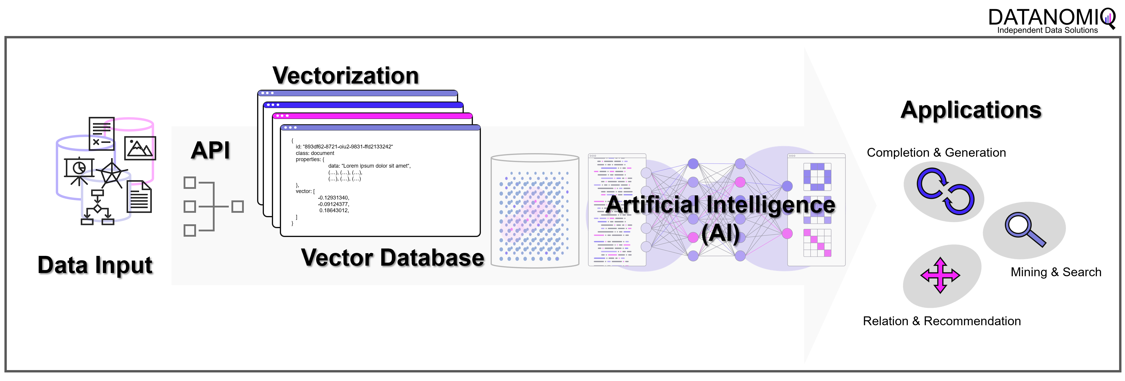
Mit der DATANOMIQ Enterprise AI Architektur, die auf jeder Cloud ausrollfähig ist, verfügen Unternehmen über einen intelligenten Unternehmens-Repräsentanten als KI, der für Mitarbeiter relevante Dokumente und Antworten auf Fragen liefert. Sollte irgendein Mitarbeiter im Unternehmen bereits einen bestimmten Vorgang, Vorfall oder z. B. eine technische Konstruktion oder einen rechtlichen Vertrag bearbeitet haben, der einem aktuellen Fall ähnlich ist, wird die AI dies aufspüren und sinnvollen Kontext, Querverweise oder Vorschläge oder lückenauffüllende Daten liefern.
Die AI lernt permanent mit, Unternehmenswissen geht nicht verloren. Das ist Wissensmanagement auf einem neuen Level, dank Vektor-Datenbanken und KI.
Big Data – Das Versprechen wurde eingelöst
/in Artificial Intelligence, Big Data, Business Analytics, Business Intelligence, Cloud, Data Engineering, Data Science, Data Warehousing, Deep Learning, Insights, Machine Learning, Main Category/by Benjamin AunkoferBig Data tauchte als Buzzword meiner Recherche nach erstmals um das Jahr 2011 relevant in den Medien auf. Big Data wurde zum Business-Sprech der darauffolgenden Jahre. In der Parallelwelt der ITler wurde das Tool und Ökosystem Apache Hadoop quasi mit Big Data beinahe synonym gesetzt. Der Guardian verlieh Apache Hadoop mit seinem Konzept des Distributed Computing mit MapReduce im März 2011 bei den MediaGuardian Innovation Awards die Auszeichnung “Innovator of the Year”. Im Jahr 2015 erlebte der Begriff Big Data in der allgemeinen Geschäftswelt seine Euphorie-Phase mit vielen Konferenzen und Vorträgen weltweit, die sich mit dem Thema auseinandersetzten. Dann etwa im Jahr 2018 flachte der Hype um Big Data wieder ab, die Euphorie änderte sich in eine Ernüchterung, zumindest für den deutschen Mittelstand. Die große Verarbeitung von Datenmassen fand nur in ganz bestimmten Bereichen statt, die US-amerikanischen Tech-Riesen wie Google oder Facebook hingegen wurden zu Daten-Monopolisten erklärt, denen niemand das Wasser reichen könne. Big Data wurde für viele Unternehmen der traditionellen Industrie zur Enttäuschung, zum falschen Versprechen.
Von Big Data über Data Science zu AI
Einer der Gründe, warum Big Data insbesondere nach der Euphorie wieder aus der Diskussion verschwand, war der Leitspruch “Shit in, shit out” und die Kernaussage, dass Daten in großen Mengen nicht viel wert seien, wenn die Datenqualität nicht stimme. Datenqualität hingegen, wurde zum wichtigen Faktor jeder Unternehmensbewertung, was Themen wie Reporting, Data Governance und schließlich dann das Data Engineering mehr noch anschob als die Data Science.
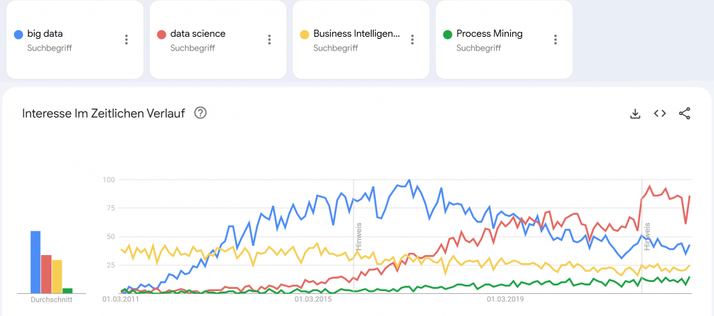
Google Trends – Big Data (blue), Data Science (red), Business Intelligence (yellow) und Process Mining (green). Quelle: https://trends.google.de/trends/explore?date=2011-03-01%202023-01-03&geo=DE&q=big%20data,data%20science,Business%20Intelligence,Process%20Mining&hl=de
Small Data wurde zum Fokus für die deutsche Industrie, denn “Big Data is messy!”1 und galt als nur schwer und teuer zu verarbeiten. Cloud Computing, erst mit den Infrastructure as a Service (IaaS) Angeboten von Amazon, Microsoft und Google, wurde zum Enabler für schnelle, flexible Big Data Architekturen. Zwischenzeitlich wurde die Business Intelligence mit Tools wie Qlik Sense, Tableau, Power BI und Looker (und vielen anderen) weiter im Markt ausgebaut, die recht neue Disziplin Process Mining (vor allem durch das deutsche Unicorn Celonis) etabliert und Data Science schloss als Hype nahtlos an Big Data etwa ab 2017 an, wurde dann ungefähr im Jahr 2021 von AI als Hype ersetzt. Von Data Science spricht auf Konferenzen heute kaum noch jemand und wurde hype-technisch komplett durch Machine Learning bzw. Artificial Intelligence (AI) ersetzt. AI wiederum scheint spätestens mit ChatGPT 2022/2023 eine neue Euphorie-Phase erreicht zu haben, mit noch ungewissem Ausgang.
Big Data Analytics erreicht die nötige Reife
Der Begriff Big Data war schon immer etwas schwammig und wurde von vielen Unternehmen und Experten schnell auch im Kontext kleinerer Datenmengen verwendet.2 Denn heute spielt die Definition darüber, was Big Data eigentlich genau ist, wirklich keine Rolle mehr. Alle zuvor genannten Hypes sind selbst Erben des Hypes um Big Data.
Während vor Jahren noch kleine Datenanalysen reichen mussten, können heute dank Data Lakes oder gar Data Lakehouse Architekturen, auf Apache Spark (dem quasi-Nachfolger von Hadoop) basierende Datenbank- und Analysesysteme, strukturierte Datentabellen über semi-strukturierte bis komplett unstrukturierte Daten umfassend und versioniert gespeichert, fusioniert, verknüpft und ausgewertet werden. Das funktioniert heute problemlos in der Cloud, notfalls jedoch auch in einem eigenen Rechenzentrum On-Premise. Während in der Anfangszeit Apache Spark noch selbst auf einem Hardware-Cluster aufgesetzt werden musste, kommen heute eher die managed Cloud-Varianten wie Microsoft Azure Synapse oder die agnostische Alternative Databricks zum Einsatz, die auf Spark aufbauen.
Die vollautomatisierte Analyse von textlicher Sprache, von Fotos oder Videomaterial war 2015 noch Nische, gehört heute jedoch zum Alltag hinzu. Während 2015 noch von neuen Geschäftsmodellen mit Big Data geträumt wurde, sind Data as a Service und AI as a Service heute längst Realität!
ChatGPT und GPT 4 sind King of Big Data
ChatGPT erschien Ende 2022 und war prinzipiell nichts Neues, keine neue Invention (Erfindung), jedoch eine große Innovation (Marktdurchdringung), die großes öffentliches Interesse vor allem auch deswegen erhielt, weil es als kostenloses Angebot für einen eigentlich sehr kostenintensiven Service veröffentlicht und für jeden erreichbar wurde. ChatGPT basiert auf GPT-3, die dritte Version des Generative Pre-Trained Transformer Modells. Transformer sind neuronale Netze, sie ihre Input-Parameter nicht nur zu Klasseneinschätzungen verdichten (z. B. ein Bild zeigt einen Hund, eine Katze oder eine andere Klasse), sondern wieder selbst Daten in ähnliche Gestalt und Größe erstellen. So wird aus einem gegeben Bild ein neues Bild, aus einem gegeben Text, ein neuer Text oder eine sinnvolle Ergänzung (Antwort) des Textes. GPT-3 ist jedoch noch komplizierter, basiert nicht nur auf Supervised Deep Learning, sondern auch auf Reinforcement Learning.
GPT-3 wurde mit mehr als 100 Milliarden Wörter trainiert, das parametrisierte Machine Learning Modell selbst wiegt 800 GB (quasi nur die Neuronen!)3.
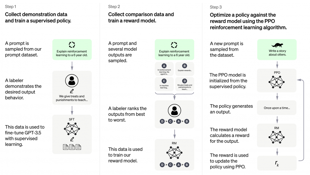
ChatGPT basiert auf GPT-3.5 und wurde in 3 Schritten trainiert. Neben Supervised Learning kam auch Reinforcement Learning zum Einsatz. Quelle: openai.com
GPT-3 von openai.com war 2021 mit 175 Milliarden Parametern das weltweit größte Neuronale Netz der Welt.4
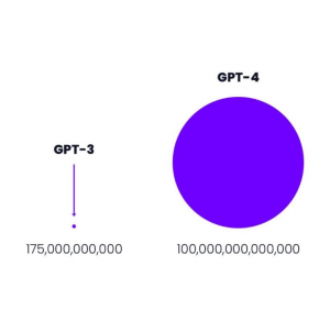
Größenvergleich: Parameteranzahl GPT-3 vs GPT-4 Quelle: openai.com
Der davor existierende Platzhirsch unter den Modellen kam von Microsoft mit “nur” 10 Milliarden Parametern und damit um den Faktor 17 kleiner. Das nun neue Modell GPT-4 ist mit 100 Billionen Parametern nochmal 570 mal so “groß” wie GPT-3. Dies bedeutet keinesfalls, dass GPT-4 entsprechend 570 mal so fähig sein wird wie GPT-3, jedoch wird der Faktor immer noch deutlich und spürbar sein und sicher eine Erweiterung der Fähigkeiten bedeuten.
Was Big Data & Analytics heute für Unternehmen erreicht
Auf Big Data basierende Systeme wie ChatGPT sollte es – der zuvor genannten Logik folgend – jedoch eigentlich gar nicht geben dürfen, denn die rohen Datenmassen, die für das Training verwendet wurden, konnten nicht im Detail auf ihre Qualität überprüft werden. Zum Einen mittelt die Masse an Daten die in ihnen zu findenden Fehler weitgehend raus, zum Anderen filtert Deep Learning selbst relevante Muster und unliebsame Ausreißer aus den Datenmassen heraus. Neuronale Netze, der Kern des Deep Learning, können durchaus als große Filter verstanden und erklärt werden.
Davon abgesehen, dass die neuen ChatBot-APIs von den Cloud-Providern Microsoft, Google und auch Amazon genutzt werden können, um Arbeitsprozesse und Kommunikation zu automatisieren, wird Big Data heute in vielen Unternehmen dazu eingesetzt, um Unternehmens-/Finanzkennzahlen auszuwerten und vorherzusagen, um Produktionsqualität zu überwachen, um Maschinen-Sensordaten mit den Geschäftsdaten aus ERP-, MES- und CRM-Systemen zu verheiraten, um operative Prozesse über mehrere IT-Systeme hinweg zu rekonstruieren und auf Schwachstellen hin zu untersuchen und um Schlussendlich auch den weiteren Datenhunger zu stillen, z. B. über Text-Extraktion aus Webseiten (Intelligence Gathering), die mit NLP und Computer Vision mächtiger wird als je zuvor.
Big Data hält sein Versprechen dank AI
Die frühere Enttäuschung aus Big Data resultierte aus dem fehlenden Vermittler zwischen Big Data (passive Daten) und den Applikationen (z. B. Industrie 4.0). Dieser Vermittler ist der aktive Part, die AI und weiterführende Datenverarbeitung (z. B. Lakehousing) und Analysemethodik (z. B. Process Mining). Davon abgesehen, dass mit AI über Big Data bereits in Medizin und im Verkehrswesen Menschenleben gerettet wurden, ist Big Data & AI längst auch in gewöhnlichen Unternehmen angekommen. Big Data hält sein Versprechen für Unternehmen doch noch ein und revolutioniert Geschäftsmodelle und Geschäftsprozesse, sichert so Wettbewerbsfähigkeit. Zumindest, wenn Unternehmen sich auf diesen Weg tatsächlich einlassen.
Quellen:
- Edd Dumbill: What is big data? An introduction to the big data landscape. (Memento vom 23. April 2014 im Internet Archive) auf: strata.oreilly.com.
↑ - Fergus Gloster: Von Big Data reden aber Small Data meinen. Computerwoche, 1. Oktober 2014↑
- Bussler, Frederik (July 21, 2020). “Will GPT-3 Kill Coding?”. Towards Data Science. Retrieved August 1, 2020.2022↑
- developer.nvidia.com, 1. Oktober 2014↑
How to tackle lack of data: an overview on transfer learning
/in Artificial Intelligence, Data Mining, Data Science, Deep Learning, Machine Learning, Predictive Analytics, Reinforcement Learning/by Yasuto Tamura1, Data is the new oil, but labeled data might be closer to it
Even though we have been in the 3rd AI boom and machine learning is showing concrete effectiveness at a commercial level, after the first two AI booms we are facing a problem: lack of labeled data or data themselves. The increasing number of papers on deep learning demonstrate that researches on AI have developed rapidly recently. If architectures of neural networks and supervised learning are all you know about deep learning, you will be overwhelmed by complications of topics studied these days, for example generative models, making more compact neural net models by for example knowledge distillation, and explainable AI (XAI). Those researches are often conducted on easily available benchmark datasets which you can easily download, often with corresponding ground truth data (label data) necessary for training. However once you try to apply the techniques to more specific data, you usually cannot prepare enough label data which theoretical researches assume. Thus among fascinating deep learning topics, in this article I am going to pick up how to tackle lack of label or data themselves, and transfer learning. Transfer learning is a technique of machine learning to take advantages of knowledge learned in one dataset to deal with a task in another dataset. Presumably due to this fact, Andrew Ng, in his presentation in NeurIPS 2016, gave a rough and abstract predictions of how transfer learning in machine learning would make commercial success like white lines in the figure below. The explanation is straightforward, and given the trends in topics of researches on machine learning these days, this prediction is actually right. But at the same time, in my opinion supervised learning, transfer learning, and unsupervised learning cannot be clearly separated like the graph originally suggested by Andrew Ng. Those fields complement each other, and one can easily shift to another.
Source: https://ruder.io/transfer-learning/ The lines and texts in white are based on explanations by Andrew Ng. The orange cells are placed at random, so not that they represent commercial success of each field.
Along with the rapid progress of deep learning mentioned above, a lot of hypes and catchphrases regarding big data and machine learning were made, and an interesting one is “Data is the new oil.” That might have been said only because big data is sources of various industries. But I would say, the characteristic is more striking in training data for machine learning. Distributions of training data for machine learning are more complicated like various energy resources besides oil in the world. Labeled data might be also like uranium. Just as uranium-235 accounting for only less than one percent of uranium in the world can be used to generate energy, only a part of massive data in the world is labeled such that they can be used for supervised machine learning. And as uranium-235 is used effectively jointly with less active uranium-238, labeled data show greater potentials with unlabeled data. And training data for machine learning have another unpleasant analogy to energy resources. Like most mainstream energy resources, only limited companies or institutions would be able to mine and refine huge labeled datasets with gigantic computation resources, and most people more or less need to rely on that for their business. Even though alternative renewable energy resources are proposed, principal energy resources are indispensable for making industries stable. As well, even though a lot of techniques actually have been proposed to lack of data, it often turns out just fine-tuning pre-trained models is the most practical, which need huge datasets and rich computational resources. And I think recent success in for example BERT or GPT made this trend more visible.
*I am sorry in a case I am mistaken about energy resources. I just wanted to come up with some cool metaphors.
But I still think knowing about transfer learning more comprehensively would be effective. That is partly because I have been working on relatively unique data which are hard to even label. As I was studying computer vision (CV) in plant science field, I frequently saw relatively unique data obtained with special apparatuses. Such data are for the most part look far from very general dataset, which huge pre-trained models are trained on. At the same time such plant data have very complicated structures and hard to label. And also in my work, have to detect certain values in various formats in very specific documents, in German. Such data are far from general datasets, and even labeling is hard in that case. We have to carefully tackle lack of data every time on each type of data in that case.
In this article I would first like to explain in the first place what it is like to lack data and next introduce representative techniques to tackle lack of labeled data. Many of them are classified to transfer learning, but other techniques like unsupervised learning or self-supervised learning are used in them or share a lot in their ideas. Thus my main purpose of writing this article is to let you have a richer view on transfer learning. And you would see “transfer learning” these days are mainly about fine-tuning of pre-trained models. Also how to tackle lack of data or labels is in other words how to efficiently achieve good performance in machine learning. Thus even if tons of high quality labeled data are at your disposal, learning those ideas would be still effective to you. I hope you could find some hints of machine learning through my articles.
2, What does lack of data or labels mean in the first place?
We need to first consider what lack of labels or data means, and my answer to the title of this section is “It depends.” The more data you have, the better performances you get. And the bigger machine learning models are, the more data they usually need for training. I assume that people reading this article more or less understand neural networks and how they are trained with back propagation. But let’s review the process here. Most machine learning frameworks are more or less expressed like the figure below unless reinforcement learning is considered. The ultimate purpose of machine learning is to train a model ![]() by adjusting parameters
by adjusting parameters ![]() . And the parameters
. And the parameters ![]() are optimized so that a loss function
are optimized so that a loss function ![]() is minimized. If it is a supervised learning, the a value of a loss function is denoted
is minimized. If it is a supervised learning, the a value of a loss function is denoted ![]()
![]() , and it gets smaller as
, and it gets smaller as ![]() gets closer to
gets closer to ![]() . That is,
. That is, ![]() is giving supervision to adjust
is giving supervision to adjust ![]() via
via ![]() . And in a case of unsupervised learning, a loss function is
. And in a case of unsupervised learning, a loss function is ![]() , which is often heuristically handcrafted.
, which is often heuristically handcrafted.

The very first problem from lacking training data you would learn is overfitting. That is, a machine learning model can be specialized too much for a training dataset, and it loses generalization to other data from the same dataset. It is like students with little imaginations and flexibility gradually memorizing all the answers in a textbook and failing to answer new questions they have not encountered yet. Overfitting is judged by relations of training and validation loss like in the graph below. Training loss in blue indicates how the students adjust to the textbook. The smaller the training loss is, the more they memorizes from the textbook and the less flexible they are. The orange line indicates their performance in newly appeared questions in tests. The smaller the validation loss is, the better the students perform on tests. Thus the students should stop learning with the textbook when the validation loss is about to increase. This is called early stopping in machine learning. And if you increase training data, the orange graph usually shifts to the right side, usually providing smaller validation loss, namely better performance. An important point is, this ideal relations of training and validation losses will not appear if sizes or expressivity of a model is not enough. Thus the more training data you use, the more parameters you need for the model to enhance its expressivity.
*Depending on sizes of training data, the curve of training loss also changes, so please bear it in mind that this graph is not correct and is very simplified.
What I said so far might sound too elementary. My point is, the more data you have, and the bigger computation resource you have, the better performance you get. In other words, machine learning has scalability with data and parameters. This characteristic is clearly observed in models in natural language processing (NLP) and computer vision (CV) like in the graphs below. When I read some papers,often I am very fascinated by their performances. But sometimes it turns out that the methods are mainly creatively in terms of how they increase training data, which is personally boring. And even if performance of GPT looks astonishing, I cannot really like them because of this simple fact.
However another important point is, conversely you don’t need to increase training data or parameters of a model once it achieves an ideal score in metrics. When you make a toy model with small training data, as long as your clients or co-researchers are already happy, that is enough. Therefore lack of data or labels has to be discussed depending on sizes of machine learning and their performances you expect. Given those points mentioned so far, my answer to the question “What does lack of data or labels mean?” would rephrased like “If your model is properly designed to reach the performance you expect and it starts overfitting, you are facing lack of data.” And such decisions basically has to be made based on experiments.
3, Types of lack of data
Even though I explained lack of labels or data is a contextual matter, the problems actually exist at any case. That is, you often fail to achieve ideas accuracy partly due to lack of training data. I would like to classify types of situations of data of label shortage as below.

We should first think about the case where lack of labels does not matter in the first place. If you can analyze data with statistical knowledge or unsupervised machine learning, just extracting data without labeling would be enough. And sometimes ad hoc analysis with simple data visualization will help your decision makings. And some dashboards made from those unlabeled data will already give you some insights into data.
The next case is that, popular machine learning fields with enough investments usually have huge datasets that huge academic institutes or companies have been preparing. For example KITTI dataset, which include labels like trajectories and depth data, is by Karlsruhe Institute of Technology and Toyota Technological Institute. Such datasets are useful for self-driving-related researches, and many types of ground truth data are provided such as odometry, depth, opticla flow, detection. This kind of data might be considered “enough” only because they are enough for training machine learning models and quantitatively evaluating them in papers, regardless of practical usefulness at a commercial level. But at any rate, popular fields with large benchmark datasets are likely to get investments for commercial uses.
Next let’s see cases of data shortage. You should also keep it in mind that there are also several types of situations of data shortage. In fact there are cases where certain labels are supposed to be scarce such as classifications of imbalanced data, for example anomaly detection, judging spam mails, or medical examination. In those problems only some percent of data are classified as “errors,” “spam,” or “disease,” and others are classified as “normal.” Just keeping classifying data into “normal” would give maybe more than 95% accuracy. But finding the rest some percent accurately is much more important. In this case model performances need to be evaluated with ROC curves, namely relations of true positives and false positives.
The next type is more related to cases assumed in transfer learning. Some data are in the first place very expensive to obtain. For example CT images have to be stored by special medical apparatuses as you know. And even if a lot of CT images are already obtained, annotating the images often needs professional skills, thus its annotations cost is high. Another case of high annotation cost is for example detection or segmentation of objects in images. Even if you can collect numerous images on the Internet, annotating bounding boxes or pixel-wise segments require a lot of time. Annotating around 1000 images for classification might be ok, but annotating them at a pixel level is really time consuming. If you have a tablet, I would like you to paint each segment of objects in a picture with different colors. And you should multiply the time spent by 80,000, as many as the training images needed for Mask R-CNN, a popular model for instance segmentation. As you can imagine, it is a huge tediou work. Even preparing some 50 labeled images for fine-tuning is paiful, and even annotations for computer vision tasks itself is also a field of deep learning.
*I would say medical image processing is a relatively popular field in CV with deep learning, and there are several famous datasets on this field.
4, An overview on ways for dealing with lack of labeled data
I am going to first roughly introduce what kind of approaches can be taken to deal with lack of labeled data or data itself, but you should also keep it in mind that they are not clearly separated. Just as I am going to explain, one type of techniques can easily shift to another type. You should flexibly switch among them depending on your situations. And also please keep it in mind that these are well-studied areas, and tons of ingenious papers are announced one after another, usually giving slight changes in their performances. Problems I point out about each technique might not be a problem anymore with recently published researches on researches currently peer-read. It is hard to prove that something does not exist. Given those points, I think it is convenient to classify technique of dealing with label or data shortage as below.

Through this article, ideas of domains are important. A domain simply means a combination of a dataset and a task with it. Transfer learning is a family of machine learning techniques to make uses of knowledge learned in a domain to another domain, and the former is called a source domain, the latter a target domain. And discrepancies between a source domain and a target domain is called a domain shift. The figure below abstractly visualize examples of domains and domain shifts. Intuitively it is easy to imagine that face a CV task and an NLP task have bigger domain shifts than domains of leaf images taken from different angles, but quantitatively evaluating domain shifts is in practice hard, and I am not going to introduce the topic because that will need a lot of mathematics.

Instead of formulating transfer learning, I would like to take learning languages as an intuitive example of transfer learning. Most people master at least one native language before learning another one. Baby brains are a kind of fantastic machine learning models, and after overcoming many obstacles they master native languages. And people take advantages of their mother tongues to learn another language. Usually they learn foreign languages by comparing structures of translated sentences. And naturally, if both a foreign language and your language have analogies like grammatical cases or genders in common, language learning would be easy. In other words, proficiency in one language is helpful in leaning some language. But it is also possible that your native language badly affects learning the second language, due to grammatical structures, pronunciations. The case of a source domain deteriorating performances in a target domain is called negative transfer and contexts of transfer learning.
*I know similarities languages are not the sole and definite barometers of effectiveness in learning foreign languages. Sizes of economy or markets in a country would also affects English language acquisition of people there. But at least it is unfair to compare for example German or Dutch people learning English with Japanese, Chinese people learning it. Unlike Eastern Asian people who have to learn thousands of characters to at least read decent texts or who use very different grammars, European people obviously can use “transfer learning” to learn English.
5, Increasing training data
When you lack data or labels, the most straightforward and often quick solution is to just increase data. The two topics I will cover in this section are mainly conducted in one domain.
Data augmentation
Data augmentation is one of the first techniques you would learn to mitigate overfitting of machine learning, which is in short caused by lack of data. The idea is very simple and it is implemented well in deep learning libraries, so I would only briefly talk about it here. The idea of data augmentation is simply transforming input data by for example flipping, rotating, zooming, changing colors. By doing so for example an input image ![]() of a butterfly below with a label of
of a butterfly below with a label of ![]() can be converted to more than 6 images. This corresponds to getting a converted
can be converted to more than 6 images. This corresponds to getting a converted ![]() in the machine learning outline in the last section. And this process is the same as increasing the size of a dataet
in the machine learning outline in the last section. And this process is the same as increasing the size of a dataet ![]() . And one point you have to be careful is, you must not change
. And one point you have to be careful is, you must not change ![]() too much to change corresponding
too much to change corresponding ![]() . For example if
. For example if ![]() is distorted too much, it cannot be recognized as
is distorted too much, it cannot be recognized as ![]() anymore even by humans. Or if you rotate an image of a digit 6 180 degrees, its becomes 9. Recent researches focus on automatically find what kind of data augmentation is effective by using for example reinforcement learning.
anymore even by humans. Or if you rotate an image of a digit 6 180 degrees, its becomes 9. Recent researches focus on automatically find what kind of data augmentation is effective by using for example reinforcement learning.
 Here let me take an example of data augmentation technique that would be contrary to your intuition. A technique named mixup literally mix up data with different classes and their labels. In classification problems, labels are expressed as one-hot vectors, that is only an element corresponding to a correct element is
 ![]() and the others are
and the others are ![]() . In a case of binary dog-or-cat classification, each label is
. In a case of binary dog-or-cat classification, each label is ![]() or
or ![]() , respectively. In data augmentation, distorting data too much is a taboo because label data is contaminated, but in mixup you literally mix up labels. Randomly choosing a two inputs
, respectively. In data augmentation, distorting data too much is a taboo because label data is contaminated, but in mixup you literally mix up labels. Randomly choosing a two inputs ![]() and a number
and a number ![]() , you prepare a input and label pair
, you prepare a input and label pair ![]() . The figure below is an example of a mixing up a cat input and a dog input, and corresponding labels. It is known augmenting training data like this improves classification performances. It is said this is partly due to machine learning models effectively learning decision boundaries. In classification ambiguous inputs are bottlenecks, so learning to giving ambiguous outputs to ambiguous inputs can enhance classification abilities.
. The figure below is an example of a mixing up a cat input and a dog input, and corresponding labels. It is known augmenting training data like this improves classification performances. It is said this is partly due to machine learning models effectively learning decision boundaries. In classification ambiguous inputs are bottlenecks, so learning to giving ambiguous outputs to ambiguous inputs can enhance classification abilities.
*One-hot-encoded labels are called hard labels, and otherwise soft labels. Recent topics in deep learning, such as lottery hypothesis, knowledge distillation, imply that whether supervising labels are hard or not is important in deep learning. Hopefully I would like to explain why little by little in my articles.
6, Active learning
Active learning is about how to annotate data and get labeled data efficiently. Labels of data do not equally contribute to enhancing machine learning models, and labels actually have qualities. Even if you give apparently similar images with the same label to machine learning models during training, the models cannot learn so much from the pair of data. You need to efficiently dig data to know its distribution by giving labels to samples. I think a good metaphor is geological survey by excavating with some boring. In order to know substances or features of ground, some earth need to be sampled with boring. But you cannot freely penetrate everywhere mainly due to costs. They need to be sampled one by one due to uncertainty about the ground.
Similar approaches are often taken in machine learning or statistics, that is estimating distributions of data with a small size of samples is an important idea. A basic idea for doing that is you sample or annotate data which decreases uncertainty of your model the most. The figure simply exhibits the idea. We want to regress a data distribution with the red curve, and the cross marks can be sampled from the distribution. And the part filled with light blue shows uncertainty of the model to predict a value of ![]() for a
for a ![]() . When you want to regress the data with as few samples as possible, data points should be sampled from the parts with great uncertainties. And by doing so, you can see that the data is regressed efficiently with few samples.
. When you want to regress the data with as few samples as possible, data points should be sampled from the parts with great uncertainties. And by doing so, you can see that the data is regressed efficiently with few samples.
We have seen that modeling uncertainty is the key to active learning, and that can be applied to annotations of data in deep learning. An example of the process is displayed below, and in this case a deep neural network model (DNN model) is trained with some labeled data, and you give some signals for data annotations based on uncertainty of outputs of DNN models. And human annotators prioritize giving labels to the data. Such uncertainly can be estimated by using entropy of outputs or modeling data distributions.
But when you get a certain amount of labels, the situation will be the same as semi-supervised learning, which I will explain next. That is, you might be already able to make the most of the labels so far with the help of unlabeled data. You should consider stopping labeling and start labeling depending on situations. And importantly, starting naively annotating data might become a quick solution rather than thinking about how to make uses of limited labels if extracting data itself is easy and does not cost so much. “Shut up and annotate!” could be often the best practice in practice. And annotations would be an effective way for exploratory data analysis (EDA), so I recommend you to immediately start annotating about 10 random samples at any rate.
7, Dealing with lack of labels in a single domain
In many cases, data themselves are easily available, and only annotations costs matter. The following two topics consider such cases, and again only one domain is considered. But by the end of this article you would see that other techniques covered in this article have a lot of analogies with topics introduced here.
Semi-supervised learning
Semi-supervised learning is a type of supervised learning where only limited labels are available in one domain. This is important in because many of other techniques in this article can be seen as semi-supervised learning from certain points of views. The figure below shows an intuition on semi-supervised learning in a case of classification task. In this case, original data distribution have two clusters of circles and triangles and a clear border can be drawn between them. But only with limited labeled data, decision boundaries would be ambiguous. However in fact, with a help of unlabeled data in dotted lines, machine learning model might be able to recognize two clusters with a help of unlabeled data. In other words, unlabeled data help models learn distribution of data. this might be natural as clusters of data can be estimated with unsupervised learning.
*As I have already mentioned, active learning could soon shift to semi-supervised learning, and it might be worth trying it before finishing labeling. But suspending labeling and resuming it later might not be efficient. At any rate you need to be flexible depending on situations.
Semi-supervised learning is applicable to several tasks, not only classification. I explained that normal supervised learning is adjusting parameters ![]() of a model
of a model ![]() so that it minimize loss function
so that it minimize loss function ![]() for a labeled dataset
for a labeled dataset ![]() . In semi-supervised learning, we assume that usually a bigger unsupervised dataset
. In semi-supervised learning, we assume that usually a bigger unsupervised dataset ![]() is available in the same domain. And semi-supervised learning optimize
is available in the same domain. And semi-supervised learning optimize ![]() by jointly minimizing
by jointly minimizing ![]() after designing a loss function
after designing a loss function ![]() for the unlabeled dataset. There are following 3 major ways of semi-supervised learning depending on how you design a
for the unlabeled dataset. There are following 3 major ways of semi-supervised learning depending on how you design a ![]() .
.
- Consistency regularization: adding slight changes to data
 in
in  and get
  . And training
  so that
  and
and  give out a consistent output.
 - Pseudo label: after training
 with
with  , using some estimations
  as labels of
  .
. - Entropy minimization: encouraging outputs
 to have smaller entropy.
More or less similar ideas show up in different transfer learning techniques, so it would be effective to learn the three semi-supervised learning ideas above.
Self-supervised learning
Self-supervised learning is often counted as unsupervised learning. Both unsupervised and self-supervised learning do not need label data, but especially when labels generated by processing themselves, that is often called self-supervised learning. A representative case of using self-supervised learning is auto-encoder. Simpler labels can be generated from input data themselves with elementary data processing. For example in a case of image processing, by rotating an input image 0, 90, 180, 270 degrees respectively, a classification task of estimating rotation degrees can be made. Another case is estimating the original input image after some simple image processing (for example colorization). These simple tasks generated solely from an input is called pretext task. And in a case of image processing, deep learning models can be prompted to learn image features .

Source: https://atcold.github.io/pytorch-Deep-Learning/en/week10/10-1/
Pretext tasks are applicable also to other fields for example NLP. A very simple task is hiding a part of an input sentence, and let neural networks estimate the blank word. And this is a basic idea of how to train BERTs, famous pre-trained NLP models. BERT models are trained this way with a huge and very general corpus without any specific topics. By doing so BERT model can already learn to detect some clusters of meanings in texts, as I visualize in the next section. But if you fine-tune BERT models with labeled texts with very specific topics, that often fails to achieve satisfying performance. In that case, the BERT models have to “get used to” the new dataset. In that case, BERT can “get used to” the new dataset by applying self-supervised learning on the new dataset. This tutorial of Huggingface demonstrates this with an example of adjusting a BERT model trained with Wikipedia to the IMDb dataset.

In the case above, the BERT model is fine-tuned with relatively lots of unlabeled data and after that trained with fewer labels. As a whole this can be seen as semi-supervised learning ,with fewer labels of the IMBb dataset and more unlabeled data. Also the ideas of pretext tasks, which prompt models to give consistent outputs given preprocessed inputs, have some analogies with consistency regularization in semi-supervised learning.
*The Huggingface tutorial says, they fine-tune a pre-trained BERT model trained in a self-supervised way to adjus it, and they call it “domain adaptation.” As you can see from the statement, distinctions of topics covered in this article can be just ambiguous.
8, Dealing with lack of data or labels over several domains
Another approach for tackling label or data shortage is taking advantages of other domains, which are usually larger and have enough labels. And such techniques is called transfer learning as I mentioned. It seems like transfer learning in business refers to “fine-tuning” explained below, but in academic contexts it is often also said transfer learning is almost synonym to “domain adaptation.” At any rate, my point is it would be more important to have comprehensive view on the techniques rather than clearly distinguishing them.
Fine tuning
Fine tuning would be the easiest way of transfer learning, and at the same time it is very powerful. Even though I am going to introduce other technique of transfer learning, more often than not it turns out that fine tuning can compensate them. Here I will only explain what it is like to use fine-tuning. I would say using fine-tuning is easy like using instant coffee. Conventionally you needed to train your original model with your own data, and that is very affected by sizes of data you have. I would say, that was like making coffee or coffee cakes from coffee you made from beans. But by using pre-trained models already trained somewhere with huge datasets, you can use models which can already more or less recognize data. The idea was very normal already in the field of CV, and NLP got the same idea with the advent of BERT, or already with word embeddings. That is like people learned to use instant coffee instead of roasting and brewing coffee every time.
How such instant coffee is made depends on which type of deep learning is used on a huge dataset. Backbone CNN is usually trained on ImageNet dataset with supervised learning of a classification task. In case of BERT, it is trained with a huge corpus with a pretext task of estimating blank words of input sentences, which is classified to self-supervised learning. Let me more practically what the “coffee syrup” means. Machine learning is at any rate just mapping of tensors or vectors. In CV, an input images as a tensor is converted into a a vector or a tensor, and tasks like image classification are conducted with the converted tensor or vector. In case of an NLP task, usually a sequence of vectors is converted to a vector or another sequence of vectors. And these resulting tensors of vectors from models are the very “coffee syrup” I am talking about. An important point is, fine-tuning also considers transfer learning between different tasks. Backbone CNNs are usually trained with classification, BERT with self-supervised learning, but the there are a variety of final tasks. They are called downstream tasks. In other words, you don’t necessarily drink instant coffee as coffee.
The two figures below are visualizations what the “instant coffee syrup” means. I processed random ![]() images in a dataset with a pre-trained backbone CNN, and I got corresponding
images in a dataset with a pre-trained backbone CNN, and I got corresponding ![]() dimensional vectors, that is a
dimensional vectors, that is a ![]() tensor. And I applied t-SNE to reduce its dimension from
tensor. And I applied t-SNE to reduce its dimension from ![]() to
to ![]() and got a
and got a ![]() tensor. The figure below shows arrangements of input images in the 2 dimensional space. As you can see, semantically similar images get closer.
tensor. The figure below shows arrangements of input images in the 2 dimensional space. As you can see, semantically similar images get closer.
Just as well, if you process random texts with BERT and apply a dimension reduction, you get a visualization like below. As well as the figure above, texts in similar topic get closer.
To make it catchy I expressed them as “coffee syrup” but this is a kind of how so-called AI sees data. Images and texts are just vectors or tensors on computer, and AI process another set of tensors of vectors in spaces which make sense to them.
Fine-tuning is quite easy. You have only to train a pre-trained model you downloaded just like normal supervised learning with your dataset. And when you train CV models with backbone CNN, the backbone is almost automatically downloaded. You have to be careful about some points, for example you have to set learning rate smaller. Let me avoid too detailed points in this article. Hopefully in the future, I’d like to write about more practical fine-tuning tips.
Domain adaptation
Domain adaptation is another family of techniques to make uses of knowledge gained in one domain in another domain. Domain adaptation is a Domain adaptation is these days often used as almost a synonym of transfer learning. But papers on domain adaptation usually assume to handle the same tasks both in a source and a target domain. So I would say domain adaptation is a subfield of transfer learning. Domain adaptation is more of how to tackle deterioration of machine learning performances when trained models are applied in different domains. Based on how much labels are available in each domain, domain adaptation is classified to several types. And unsupervised domain adaptation (UDA), where labels are available only in a source domain, is considered as the most challenging and studied well.
*Another explanation I often hear about domain adaptation is, when a models trained on a dataset is trained on another data, domain adaptation can be used to mitigate decreases in performance. I think in this context, performance of the model on the source domain is not discussed. When you apply some retraining with a new dataset, performance of the model on the source domain often drastically decrease. This is called catastrophic forgetting, and techniques like continuous learning are studied to tackle this problem. I have not really seen continuous learning in contexts of domain adaptation, but I thin these are related.
There several approaches in domain adaptation, and one frequently used approach is using adversarial loss. As we saw with the example of getting “coffee syrup,” data is first mapped into a certain space, and this is often called feature extraction. And outputs with the feature extractor are processed are processed more to give task-specific results with some networks. Often in domain adaptation, we put a domain discriminator network right after the feature extractor. And the domain discriminator classifies whether the features extracted come from the source or target domain. The feature extractor tries to extract features the domain have in common, and the domain discriminator tries to distinguish them, and two networks compete. In this way, the feature extractor and the domain discriminator form generative adversarial network (GAN), and the feature extractor learns to extract features that are hard to distinguish their domains. Feature extractor is trained so that it extract domain invariant features, for example edges and silhouette.

As well as in other transfer learning techniques, one ultimate goal of UDA is training a deep learning model only with synthetic labeled data, for example CGI, and apply the model on a totally unlabeled dataset. Converting a source domain to look like a target domain with Cycle GAN is an often used approach in domain adaptation. In domain adaptation a source domain is supposed to be easier to annotate. The figure below is an example of converting a black and white cell images to colored images.
*You could easily try converting data with Cycle GAN by preparing two datasets, and I made the converted data by myself. But you need at least one GPU to try that.

However some people insist that usefulness of UDA is very questionable. In the first place, if you do not have any labels on the target domain, that means you cannot evaluate anything qualitatively on the dataset of interest. And if you can prepare some of evaluation data or labels, applying other techniques like fine-tuning might be enough.
Meta learning and few-shot learning
One simple way to explain meta learning is that, it is a machine learning technique teach models to learn efficiently. We can also say that it is a transfer learning case where target domains are unknown. A famous meta learning method is Model-Agnostic Meta-Learning (MAML). MAML is used to get an ideal parameter ![]() which can be quickly and effectively used to new tasks. Like in the figure below,
which can be quickly and effectively used to new tasks. Like in the figure below, ![]() reaches the generally convenient parameter shown as the black dot. And the parameter can quickly reach the parameters
reaches the generally convenient parameter shown as the black dot. And the parameter can quickly reach the parameters ![]() , which effective for each task.
, which effective for each task. 
Another interesting application of meta learning is few-shot learning. Few-shot learning trains a classification model to learn to acquire classification ability based only on a very few samples. By letting the models learn classification tasks over many episodes, the model learn comes to learn efficiently from limited data samples at a test phase. The figure below shows a case of few-shot learning, where a model learns some episodes of 3-class classifications with only 4 samples per class. Few-shot learning attempts to enable human-level flexibility of perception. MAML is known to be effective also for few-shot learning.
However, studies these days do also show that fine tuning pre-trained models with a few sample data show competitive results to those by few-shot learning. Similar things can be said about large language models like GPT. Chat GPT or GPT-3/GPT-4 for example can be fine-tuned with small extra training samples, and the logic behind is different from meta learning. Fine-tuning pre-trained models rather might be closer to human learning. Humans can effectively learn new topics based on what they have experienced so far. Thus again here, fine-tuning models can be an easier and realistic solution.
I have explained an overview of machine learning techniques for handling lack of data, and as you might have noticed, fine-tuning models could be enough in many cases. I am not sure how much other transfer learning technique would be widely as useful as fine-tuning at a business level. At least, I hope this article would be a rough guideline for machine learning tasks with small sizes of data or labels. And if you have a chance to work on very unique data with very few labels, you wouldn’t be able to rely so much on only naive fine tuning of pre-trained models. In that case, you tasks have your own problem, and you would have to be careful about your EDA, data cleaning, and labeling. In that case you should consider some techniques introduced here. Hopefully someday I would like to write more detailed tutorials with each transfer learning technique. And I hope you would be able to apply a variety of transfer learning locally, not only relying on huge resources of gigantic entities. And that would lead to a more secure future, I guess.
Interesting links
Here are some interesting links for you! Enjoy your stay :)Pages
- @Data Science Blog
- authors
- Autor werden!
- Become an Author
- Bootcamp Datenanalyse und Maschinelles Lernen mit Python
- CIO Interviews
- Computational and Data Science
- Coursera Data Science Specialization
- Coursera 用Python玩转数据 Data Processing Using Python
- Data Leader Day 2016 – Rabatt für Data Scientists!
- Data Science
- Data Science Business Professional
- Data Science Insights
- Data Science Partner
- DATANOMIQ Big Data & Data Science Seminare
- DATANOMIQ Process Mining Workshop
- DATANOMIQ Seminare für Führungskräfte
- DataQuest.io – Interactive Learning
- Datenschutz
- Donation / Spende
- Education / Certification
- Fraunhofer Academy Zertifikatsprogramm »Data Scientist«
- Für Presse / Redakteure
- HARVARD Data Science Certificate Courses
- Home
- Impressum / Imprint
- MapR Big Data Expert
- Masterstudiengang Data Science
- Masterstudiengang Management & Data Science
- MongoDB University Online Courses
- Newsletter
- O’Reilly Video Training – Data Science with R
- Products
- qSkills Workshop: Industrial Security
- Science Digital Intelligence & Marketing Analytics
- Show your Desk!
- Stanford University Online -Statistical Learning
- Top Authors
- TU Chemnitz – Masterstudiengang Business Intelligence & Analytics
- TU Dortmund – Datenwissenschaft – Master of Science
- TU Dortmund berufsbegleitendes Zertifikatsstudium
- Weiterbildung mit Hochschulzertifikat Data Science & Business Analytics für Einsteiger
- WWU Münster – Zertifikatsstudiengang “Data Science”
- Zertifikatskurs „Data Science“
- Zertifizierter Business Analyst
Categories
- Apache Spark
- Artificial Intelligence
- Audit Analytics
- Big Data
- Books
- Business Analytics
- Business Intelligence
- Carrier
- Certification / Training
- Cloud
- Cloud
- Connected Car
- Customer Analytics
- Data Engineering
- Data Migration
- Data Mining
- Data Science
- Data Science at the Command Line
- Data Science Hack
- Data Science News
- Data Security
- Data Warehousing
- Database
- Datacenter
- Deep Learning
- Devices
- DevOps
- Education / Certification
- ETL
- Events
- Excel / Power BI
- Experience
- Gerneral
- GPU-Processing
- Graph Database
- Hacking
- Hadoop
- Hadoop Framework
- Industrie 4.0
- Infrastructure as Code
- InMemory
- Insights
- Interview mit CIO
- Interviews
- Java
- JavaScript
- Jobs
- Machine Learning
- Main Category
- Manufacturing
- Mathematics
- Mobile Device Management
- Mobile Devices
- Natural Language Processing
- Neo4J
- NoSQL
- Octave
- optimization
- Predictive Analytics
- Process Mining
- Projectmanagement
- Python
- Python
- R Statistics
- Re-Engineering
- Realtime Analytics
- Recommendations
- Reinforcement Learning
- Scala
- Software Development
- Sponsoring Partner Posts
- SQL
- Statistics
- TensorFlow
- Terraform
- Text Mining
- Tool Introduction
- Tools
- Tutorial
- Uncategorized
- Use Case
- Use Cases
- Visualization
- Web- & App-Tracking
Archive
- March 2025
- December 2024
- October 2024
- September 2024
- August 2024
- July 2024
- May 2024
- April 2024
- March 2024
- February 2024
- January 2024
- November 2023
- October 2023
- September 2023
- August 2023
- July 2023
- June 2023
- May 2023
- April 2023
- March 2023
- February 2023
- January 2023
- December 2022
- November 2022
- October 2022
- September 2022
- August 2022
- July 2022
- June 2022
- May 2022
- April 2022
- March 2022
- February 2022
- January 2022
- December 2021
- November 2021
- October 2021
- September 2021
- August 2021
- July 2021
- June 2021
- May 2021
- April 2021
- March 2021
- February 2021
- January 2021
- December 2020
- November 2020
- October 2020
- September 2020
- August 2020
- July 2020
- June 2020
- May 2020
- April 2020
- March 2020
- February 2020
- January 2020
- December 2019
- November 2019
- October 2019
- September 2019
- August 2019
- July 2019
- June 2019
- May 2019
- April 2019
- March 2019
- February 2019
- January 2019
- December 2018
- November 2018
- October 2018
- September 2018
- August 2018
- July 2018
- June 2018
- May 2018
- April 2018
- March 2018
- February 2018
- January 2018
- December 2017
- November 2017
- October 2017
- September 2017
- August 2017
- July 2017
- June 2017
- May 2017
- April 2017
- March 2017
- February 2017
- January 2017
- December 2016
- November 2016
- October 2016
- September 2016
- August 2016
- July 2016
- June 2016
- May 2016
- April 2016
- March 2016
- February 2016
- January 2016
- December 2015
- November 2015
- October 2015
- September 2015
- August 2015
- July 2015
- June 2015
- May 2015


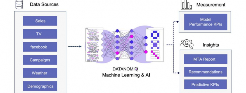 DATANOMIQ

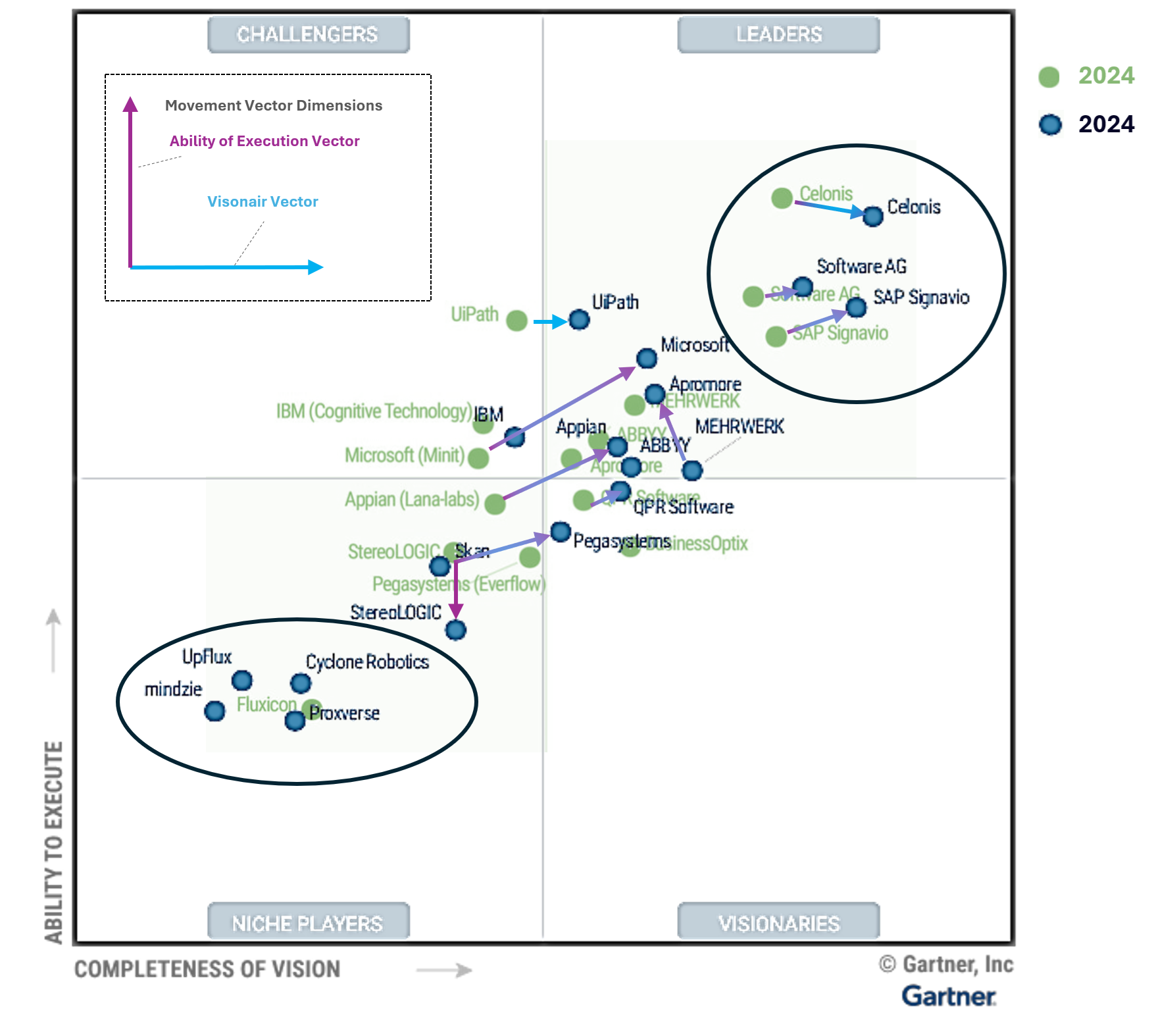


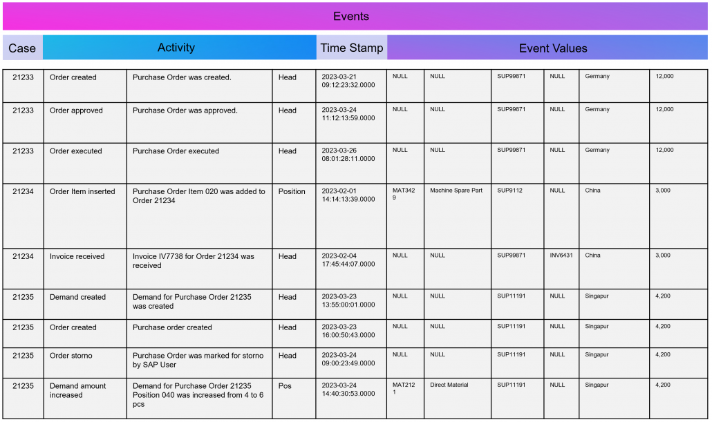
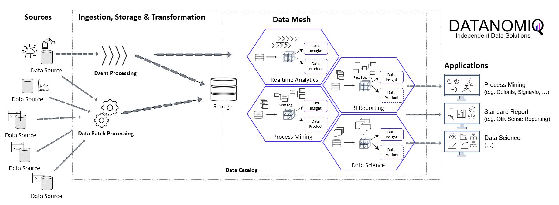
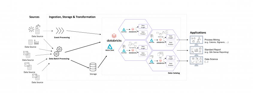
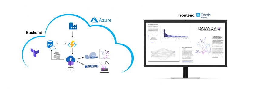
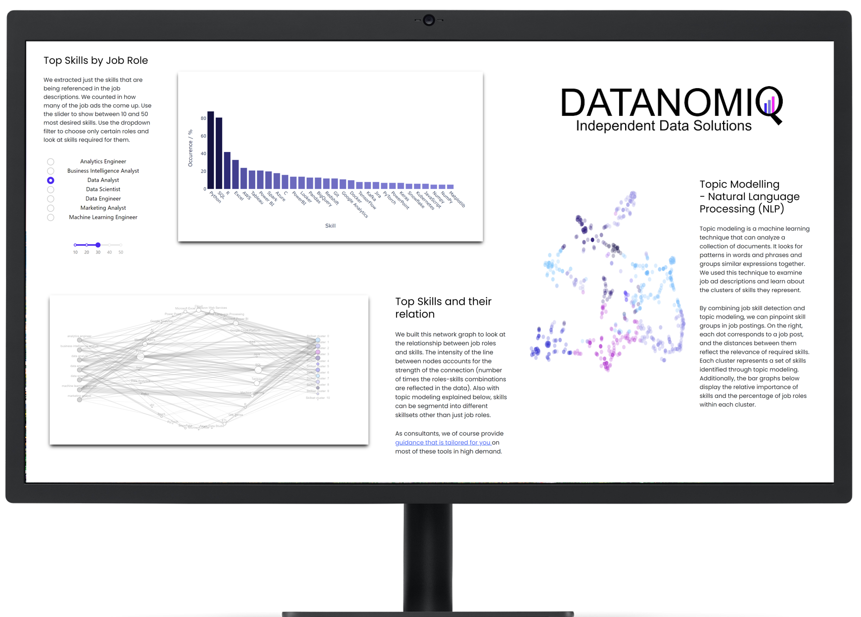
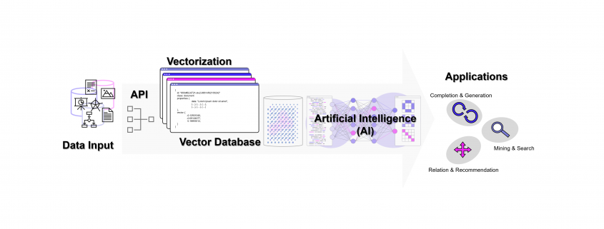 DATANOMIQ - Benjamin Aunkofer