Instructions on Transformer for people outside NLP field, but with examples of NLP

December 30, 2020/in Artificial Intelligence, Data Mining, Data Science, Deep Learning, Machine Learning, Main Category, Mathematics, Natural Language Processing, Predictive Analytics/by Yasuto Tamura

I found it quite difficult to explain mathematical details of long short-term memory (LSTM) in my previous article series. But when I was studying LSTM, a new promising algorithm was already attracting attentions. The algorithm is named Transformer. Its algorithm was a first announced in a paper named “Attention Is All You Need,” and it outperformed conventional translation algorithms with lower computational costs.

In this article series, I am going to provide explanations on minimum prerequisites for understanding deep learning in NLP (natural language process) tasks, but NLP is not the main focus of this article series, and actually I do not study in NLP field. I think Transformer is going to be a new major model of deep learning as well as CNN or RNN, and the model is now being applied in various fields.

Even though Transformer is going to be a very general deep learning model, I still believe it would be an effective way to understand Transformer with some NLP because language is a good topic we have in common. Unlike my previous article series, in which I tried to explain theoretical side of RNN as precisely as possible, in this article I am going to focus on practical stuff with my toy implementations of NLP tasks, largely based on Tensorflow official tutorial. But still I will do my best to make it as straightforward as possible to understand the architecture of Transformer with various original figures.

This series is going to be composed of the articles below.

On the difficulty of language: prerequisites for NLP with Transformer
Seq2seq model and attention mechanism: a backbone of NLP with deep learning
Multi-head attention: the key component of Transformer
Positional encoding, residual connections, padding masks: covering the rest of Transformer components
How to make a toy English-German translator with multi-head attention heat maps: the overall architecture of Transformer
Transformer in image processing (Coming soon)

If you are in the field and can read the codes in the official tutorial with no questions, this article series is not for you, but if you want to see how a Transformer works but do not want to go too much into details of NLP, this article would be for you.

The algorithm known as PCA and my taxonomy of linear dimension reductions

November 23, 2020/in Artificial Intelligence, Big Data, Data Mining, Data Science, Machine Learning, Main Category, Mathematics, Statistics/by Yasuto Tamura

In one of my previous articles, I explained the importance of reducing dimensions. Principal Component Analysis (PCA) and Linear Discriminant Analysis (LDA) are the simplest types of dimension reduction algorithms. In upcoming articles of mine, you are going to see what these algorithms do. In conclusion, diagonalization, which I mentioned in the last article, is what these algorithms are all about, but still in this article I can mainly cover only PCA.

This article is largely based on the explanations in Pattern Recognition and Machine Learning by C. M. Bishop (which is often called “PRML”), and when you search “PCA” on the Internet, you will find more or less similar explanations. However I hope I can go some steps ahead throughout this article series. I mean, I am planning to also cover more generalized versions of PCA, meanings of diagonalization, the idea of subspace. I believe this article series is also effective for refreshing your insight into linear algebra.

*This is the third article of my article series “Illustrative introductions on dimension reduction.”

1. My taxonomy on linear dimension reduction

*If you soon want to know what the algorithm called “PCA” is, you should skip this section for now to avoid confusion.

Out of the two algorithms I mentioned, PCA is especially important and you would see the same or similar ideas in various fields such as signal processing, psychology, and structural mechanics. However in most cases, the word “PCA” refers to one certain algorithm of linear dimension reduction. Most articles or study materials only mention the “PCA,” and this article is also going to cover only the algorithm which most poeple call “PCA.” However I found that PCA is only one branch of linear dimension reduction algorithms.

*From now on all the terms “PCA” in this article means the algorithm known as PCA unless I clearly mention the generalized KL transform.

*This chart might be confusing to you. According to PRML, PCA and KL transform is identical. PCA has two formulations, maximum variance formulation and minimum error formulation, and they can give the same result. However according to a Japanese textbook, which is very precise about this topic, KL transform has two formulations, and what we call PCA is based on maximum variance formulation. I am still not sure about correct terminology, but in this article I am going to call the most general algorithm “generalized KL transform,” I mean the root of the chart above.

*Most materials just explain the most major PCA, but if you consider this generalized KL transform, I can introduce an intriguing classification algorithm called subspace method. This algorithm was invented in Japan, and this is not so popular in machine learning textbooks in general, but learning this method would give you better insight into the idea of multidimensional space in machine learning. In the future, I am planning to cover this topic in this article series.

2. PCA

When someones mention “PCA,” I am sure for the most part that means the algorithm I am going to explain in the rest of this article. The most intuitive and straightforward way to explain PCA is that, PCA (Principal Component Analysis) of two or three dimensional data is fitting an oval to two dimensional data or fitting an ellipsoid to three dimensional data. You can actually try to plot some random dots on a piece of paper, and draw an oval which fits the dots the best. Assume that you have these 2 or 3 dimensional data below, and please try to put an oval or an ellipsoid to the data.

I think this is nothing difficult, but I have a question: what was the logic behind your choice?

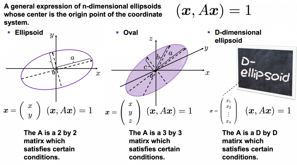
Some might have roughly drawn its outline. Formulas of “the surface” of general ellipsoids can be explained in several ways, but in this article you only have to consider ellipsoids whose center is the origin point of the coordinate system. In PCA you virtually shift data so that the mean of the data comes to the origin point of the coordinate system. When $A$ is a certain type of $D\times D$ matrix, the formula of a D-dimensional ellipsoid whose center is identical to the origin point is as follows: $(\boldsymbol{x}, A\boldsymbol{x}) = 1$ , where $\boldsymbol{x}\in \mathbb{R}$ . As is always the case with formulas in data science, you can visualize such ellipsoids if you are talking about 1, 2, or 3 dimensional data like in the figure below, but in general D-dimensional space, it is theoretical/imaginary stuff on blackboards.

*In order to explain the conditions which the matrix $A$ has to hold, I need another article, so for now please just assume that the $A$ is a kind of magical matrix.

You might have seen equations of 2 or 3 dimensional ellipsoids in the following way: $\frac{x^2}{a^2} + \frac{y^2}{b^2} = 1$ , where $a\neq 0, b\neq 0$ or $\frac{x^2}{a^2} + \frac{y^2}{b^2} + \frac{z^2}{c^2}= 1$ , where $a\neq 0, b\neq 0, c \neq 0$ . These are special cases of the equation $(\boldsymbol{x}, A\boldsymbol{x}) = 1$ , where $A=diag(a_1^2, \dots, a_D^2)$ . In this case the axes of ellipsoids the same as those of the coordinate system. Thus in this simple case, $A=diag(a^2, b^2)$ or $A=diag(a^2,c^2,c^2)$ .

I am going explain these equations in detail in the upcoming articles. But thre is one problem: how would you fit an ellipsoid when a data distribution does not look like an ellipsoid?

In fact we have to focus more on another feature of ellipsoids: all the axes of an ellipsoid are orthogonal. In conclusion the axes of the ellipsoids are more important in PCA, so I do want you to forget about the surface of ellipsoids for the time being. You might get confused if you also think about the surface of ellipsoid now. I am planning to cover this topic in the next article. I hope this article, combined with the last one and the next one, would help you have better insight into the ideas which frequently appear in data science or machine learning context.

3. Fitting orthogonal axes on data

*If you have no trouble reading the chapter 12.1 of PRML, you do not need to this section or maybe even this article, but I hope at least some charts or codes of mine would enhance your understanding on this topic.

*I must admit I wrote only the essence of PCA formulations. If that seems too abstract to you, you should just breifly read through this section and go to the next section with a more concrete example. If you are confused, there should be other good explanations on PCA on the internet, and you should also check them. But at least the visualization of PCA in the next section would be helpful.

As I implied above, all the axes of ellipsoids are orthogonal, and selecting the orthogonal axes which match data is what PCA is all about. And when you choose those orthogonal axes, it is ideal if the data look like an ellipsoid. Simply putting we want the data to “swell” along the axes.

Then let’s see how to let them “swell,” more mathematically. Assume that you have 2 dimensional data plotted on a coordinate system $(\boldsymbol{e}_1, \boldsymbol{e}_2)$ as below (The samples are plotted in purple). Intuitively, the data “swell” the most along the vector $\boldsymbol{u}_1$ . Also it is clear that $\boldsymbol{u}_2$ is the only vector orthogonal to $\boldsymbol{u}_1$ . We can expect that the new coordinate system $(\boldsymbol{u}_1, \boldsymbol{u}_2)$ expresses the data in a better way, and you you can get new coordinate points of the samples by projecting them on new axes as done with yellow lines below.

Next, let’s think about a case in 3 dimensional data. When you have 3 dimensional data in a coordinate system $(\boldsymbol{e}_1, \boldsymbol{e}_2,\boldsymbol{e}_3)$ as below, the data “swell” the most also along $\boldsymbol{u}_1$ . And the data swells the second most along $\boldsymbol{u}_2$ . The two axes, or vectors span the plain in purple. If you project all the samples on the plain, you will get 2 dimensional data at the right side. It is important that we did not consider the third axis. That implies you might be able to display the data well with only 2 dimensional sapce, which is spanned by the two axes $\boldsymbol{v}_1, \boldsymbol{v}_2$ .

Thus the problem is how to calculate such axis $\boldsymbol{u}_1$ . We want the variance of data projected on $\boldsymbol{u}_1$ to be the biggest. The coordinate of $\boldsymbol{x}_n$ on the axis $\boldsymbol{u}_1$ . The coordinate of a data point $\boldsymbol{x}_n$ on the axis $\boldsymbol{u}_1$ is calculated by projecting $\boldsymbol{x}_n$ on $\boldsymbol{u}_1$ . In data science context, such projection is synonym to taking an inner product of $\boldsymbol{x}_n$ and $\boldsymbol{u}_1$ , that is calculating $\boldsymbol{u}_1^T \boldsymbol{x}_n$ .

*Each element of $\boldsymbol{x}_n$ is the coordinate of the data point $\boldsymbol{x}_n$ in the original coordinate system. And the projected data on $\boldsymbol{u}_1$ whose coordinates are 1-dimensional correspond to only one element of transformed data.

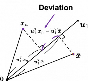
To calculate the variance of projected data on $\boldsymbol{u}_1$ , we just have to calculate the mean of variances of 1-dimensional data projected on $\boldsymbol{u}_1$ . Assume that $\bar{\boldsymbol{x}}$ is the mean of data in the original coordinate, then the deviation of $\boldsymbol{x}_1$ on the axis $\boldsymbol{u}_1$ is calculated as $\boldsymbol{u}_1^T \boldsymbol{x}_n - \boldsymbol{u}_1^T \bar{\boldsymbol{x}}$ , as shown in the figure. Hence the variance, I mean the mean of the deviation on is $\frac{1}{N} \sum^{N}_{n}{\boldsymbol{u}_1^T \boldsymbol{x}_n - \boldsymbol{u}_1^T \bar{\boldsymbol{x}}}$ , where $N$ is the total number of data points. After some deformations, you get the next equation $\frac{1}{N} \sum^{N}_{n}{\boldsymbol{u}_1^T \boldsymbol{x}_n - \boldsymbol{u}_1^T \bar{\boldsymbol{x}}} = \boldsymbol{u}_1^T S \boldsymbol{u}_1$ , where $S = \frac{1}{N}\sum_{n=1}^{N}{(\boldsymbol{x}_n - \bar{\boldsymbol{x}})(\boldsymbol{x}_n - \bar{\boldsymbol{x}})^T}$ . $S$ is known as a covariance matrix.

We are now interested in maximizing the variance of projected data on $\boldsymbol{u}_1^T S \boldsymbol{u}_1$ , and for mathematical derivation we need some college level calculus, so if that is too much for you, you can skip reading this part till the next section.

We now want to calculate $\boldsymbol{u}_1$ with which $\boldsymbol{u}_1^T S \boldsymbol{u}_1$ is its maximum value. General $\boldsymbol{u}_i$ including $\boldsymbol{u}_1$ are just coordinate axes after PCA, so we are just interested in their directions. Thus we can set one constraint $\boldsymbol{u}_1^T \boldsymbol{u}_1 = 1$ . Introducing a Lagrange multiplier, we have only to optimize next problem: $\boldsymbol{u}_1 ^ {*} = \mathop{\rm arg~max}\limits_{\boldsymbol{u}_1} \{ \boldsymbol{u}_1^T S \boldsymbol{u}_1 + \lambda_1 (1 - \boldsymbol{u}_1^T \boldsymbol{u}_1) \}$ . In conclusion $\boldsymbol{u}_1 ^ {*}$ satisfies $S\boldsymbol{u}_1 ^ {*} = \lamba_1 \boldsymbol{u}_1 ^ {*}$ . If you have read my last article on eigenvectors, you wold soon realize that this is an equation for calculating eigenvectors, and that means $\boldsymbol{u}_1 ^ {*}$ is one of eigenvectors of the covariance matrix S. Given the equation of eigenvector the next equation holds $\boldsymbol{u}_1 ^ {*}^T S \boldsymbol{u}_1 ^ {*} = \lambda_1$ . We have seen that $\boldsymbol{u}_1 ^T S \boldsymbol{u}_1 ^$ is a the variance of data when projected on a vector $\boldsymbol{u}_1$ , thus the eigenvalue $\lambda_1$ is the biggest variance possible when the data are projected on a vector.

Just in the same way you can calculate the next biggest eigenvalue $\lambda_2$ , and it it the second biggest variance possible, and in this case the date are projected on $\boldsymbol{u}_2$ , which is orthogonal to $\boldsymbol{u}_1$ . As well you can calculate orthogonal 3rd 4th …. Dth eigenvectors.

*To be exact I have to explain the cases where we can get such D orthogonal eigenvectors, but that is going to be long. I hope I can to that in the next article.

4. Practical three dimensional example of PCA

We have seen that PCA is sequentially choosing orthogonal axes along which data points swell the most. Also we have seen that it is equal to calculating eigenvalues of the covariance matrix of the data from the largest to smallest one. From now on let’s work on a practical example of data. Assume that we have 30 students’ scores of Japanese, math, and English tests as below.

* I think the subject “Japanese” is equivalent to “English” or “language art” in English speaking countries, and maybe “Deutsch” in Germany. This example and the explanation are largely based on a Japanese textbook named 「これなら分かる応用数学教室　最小二乗法からウェーブレットまで」. This is a famous textbook with cool and precise explanations on mathematics for engineering. Partly sharing this is one of purposes of this article.

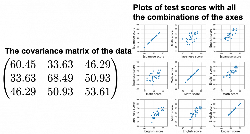
At the right side of the figure below is plots of the scores with all the combinations of coordinate axes. In total 9 inverse graphs are symmetrically arranged in the figure, and it is easy to see that English & Japanese or English and math have relatively high correlation. The more two axes have linear correlations, the bigger the covariance between them is.

In the last article, I visualized the eigenvectors of a $3\times 3$ matrix $A = \frac{1}{50} \begin{pmatrix} 60.45 & 33.63 & 46.29 \\33.63 & 68.49 & 50.93 \\ 46.29 & 50.93 & 53.61 \end{pmatrix}$ , and in fact the matrix is just a constant multiplication of this covariance matrix. I think now you understand that PCA is calculating the orthogonal eigenvectors of covariance matrix of data, that is diagonalizing covariance matrix with orthonormal eigenvectors. Hence we can guess that covariance matrix enables a type of linear transformation of rotation and expansion and contraction of vectors. And data points swell along eigenvectors of such matrix.

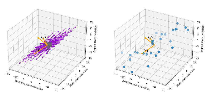
Then why PCA is useful? In order to see that at first, for simplicity assume that $x, y, z$ denote Japanese, Math, English scores respectively. The mean of the data is $\left( \begin{array}{c} \bar{x} \\ \bar{y} \\ \bar{z} \end{array} \right) = \left( \begin{array}{c} 58.1 \\ 61.8 \\ 67.3 \end{array} \right)$ , and the covariance matrix of data in the original coordinate system is $V_{xyz} = \begin{pmatrix} 60.45 & 33.63 & 46.29 \\33.63 & 68.49 & 50.93 \\ 46.29 & 50.93 & 53.61 \end{pmatrix}$ . The eigenvalues of $V_{xyz}$ are $\lambda_1=148.34, \lambda_2 = 30.62$ , and $\lambda_3 = 3.60$ , and their corresponding unit eigenvectors are $\boldsymbol{u}_1 = \left( \begin{array}{c} 0.540 \\ 0.602 \\ 0.589 \end{array} \right) , \boldsymbol{u}_2 = \left( \begin{array}{c} 0.736 \\ -0.677 \\ 0.0174 \end{array} \right) , \boldsymbol{u}_3 = \left( \begin{array}{c} -0.408 \\ -0.4.23 \\ 0.809 \end{array} \right)$ respectively. $U = (\boldsymbol{u}_1 \quad \boldsymbol{u}_2 \quad \boldsymbol{u}_3 )$ is an orthonormal matrix, where $\boldsymbol{u}_i^T\boldsymbol{u}_j = \begin{cases} 1 & (i=j) \\ 0 & (otherwise) \end{cases}$ . As I explained in the last article, you can diagonalize $V_{xyz}$ with $U$ : $U^T V_{xyz}U = diag(\lambda_1, \dots, \lambda_D)$ .

In order to see how PCA is useful, assume that $\left( \begin{array}{c} \xi \\ \eta \\ \zeta \end{array} \right) = U^T \left( \begin{array}{c} x - \bar{x} \\ y - \bar{y} \\ z - \bar{z} \end{array} \right)$ .

Let’s take a brief look at what a linear transformation by $U^T$ means. Each element of $\boldsymbol{x}$ denotes coordinate of the data point $\boldsymbol{x}$ in the original coordinate system (In this case the original coordinate system is composed of $\boldsymbol{e}_1, \boldsymbol{e}_2$ , and $\boldsymbol{e}_3$ ). $U = (\boldsymbol{u}_1, \boldsymbol{u}_2, \boldsymbol{u}_3)$ enables a rotation of a rigid body, which means the shape or arrangement of data will not change after the rotation, and $U^T$ enables a reverse rotation of the rigid body.

*Roughly putting, if you hold a bold object such as a metal ball and rotate your arm, that is a rotation of a rigid body, and your shoulder is the origin point. On the other hand, if you hold something soft like a marshmallow, it would be squashed in your hand, and that is not a not a rotation of a rigid body.

You can rotate $\boldsymbol{x}$ with $U$ like $U^T\boldsymbol{x} = \left( \begin{array}{c} -\boldsymbol{u}_1^{T}- \\ -\boldsymbol{u}_2^{T}- \\ -\boldsymbol{u}_3^{T}- \end{array} \right)\boldsymbol{x}=\left( \begin{array}{c} \boldsymbol{u}_1^{T}\boldsymbol{x} \\ \boldsymbol{u}_2^{T}\boldsymbol{x} \\ \boldsymbol{u}_3^{T}\boldsymbol{x} \end{array} \right)$ , and $\boldsymbol{u}_i^{T}\boldsymbol{x}$ is the coordinate of $\boldsymbol{x}$ projected on the axis $\boldsymbol{u}_i$ .

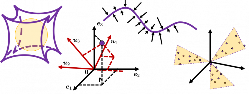
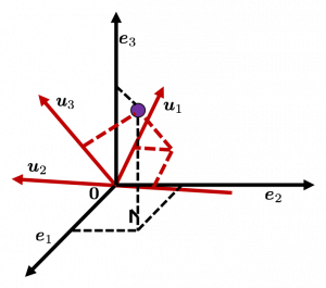
Let’s see this more visually. Assume that the data point $\boldsymbol{x}$ is a purple dot and its position is expressed in the original coordinate system spanned by black arrows . By multiplying $\boldsymbol{x}$ with $U^T$ , the purple point $\boldsymbol{x}$ is projected on the red axes respectively, and the product $\left( \begin{array}{c} \boldsymbol{u}_1^{T}\boldsymbol{x} \\ \boldsymbol{u}_2^{T}\boldsymbol{x} \\ \boldsymbol{u}_3^{T}\boldsymbol{x} \end{array} \right)$ denotes the coordinate point of the purple point in the red coordinate system. $\boldsymbol{x}$ is rotated this way, but for now I think it is better to think that the data are projected on new coordinate axes rather than the data themselves are rotating.

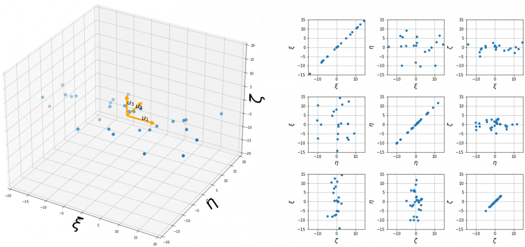
Now that we have seen what rotation by $U$ means, you should have clearer image on what $\left( \begin{array}{c} \xi \\ \eta \\ \zeta \end{array} \right) = U^T \left( \begin{array}{c} x - \bar{x} \\ y - \bar{y} \\ z - \bar{z} \end{array} \right)$ means. $\left( \begin{array}{c} \xi \\ \eta \\ \zeta \end{array} \right)$ denotes the coordinates of data projected on new axes $\boldsymbol{u}_1, \boldsymbol{u}_2, \boldsymbol{u}_3$ , which are unit eigenvectors of $V_{xyz}$ . In the coordinate system spanned by the eigenvectors, the data distribute like below.

By multiplying $U$ from both sides of the equation above, we get $\left( \begin{array}{c} x - \bar{x} \\ y - \bar{y} \\ z - \bar{z} \end{array} \right) =U \left( \begin{array}{c} \xi \\ \eta \\ \zeta \end{array} \right)$ , which means you can express deviations of the original data as linear combinations of the three factors $\xi, \eta$ , and $\zeta$ . We expect that those three factors contain keys for understanding the original data more efficiently. If you concretely write down all the equations for the factors: $\xi = 0.540 (x - \bar{x}) + 0.602 (y - \bar{y}) + 0.588 (z - \bar{z})$ , $\eta = 0.736(x - \bar{x}) - 0.677 (y - \bar{y}) + 0.0174 (z - \bar{z})$ , and $\zeta = - 0.408 (x - \bar{x}) - 0.423 (y - \bar{y}) + 0.809(z - \bar{z})$ . If you examine the coefficients of the deviations $(x - \bar{x}), (y - \bar{y})$ , and $(z - \bar{z})$ , we can observe that $\eta$ almost equally reflects the deviation of the scores of all the subjects, thus we can say $\eta$ is a factor indicating one’s general academic level. When it comes to $\eta$ Japanese and Math scores are important, so we can guess that this factor indicates whether the student is at more of “scientific side” or “liberal art side.” In the same way $\zeta$ relatively makes much of one’s English score, so it should show one’s “internationality.” However the covariance of the data $\xi, \eta, \zeta$ is $V_{\xi \eta \zeta} = \begin{pmatrix} 148.34 & 0 & 0 \\ 0 & 30.62 & 0 \\ 0 & 0 & 3.60 \end{pmatrix}$ . You can see $\zeta$ does not vary from students to students, which means it is relatively not important to describe the tendency of data. Therefore for dimension reduction you can cut off the factor $\zeta$ .

*Assume that you can apply PCA on D-dimensional data and that you get $\boldsymbol{x}'$ , where $\boldsymbol{x}' = U^T\boldsymbol{x} - \bar{\boldsymbol{x}}$ . The variance of data projected on new D-dimensional coordinate system is $V'=\frac{1}{N}\sum{(\boldsymbol{x}')^T\boldsymbol{x}'}$ $=\frac{1}{N}\sum{(U^T\boldsymbol{x})^T(U^T\boldsymbol{x})}$ $=\frac{1}{N}\sum{U^T\boldsymbol{x}\boldsymbol{x}^TU}$ $=U^T(\frac{1}{N}\sum{\boldsymbol{x}\boldsymbol{x}^T})U$ $=U^TVU$ $=diag(\lambda_1, \dots, \lambda_D)$ . This means that in the new coordinate system after PCA, covariances between any pair of variants are all zero.

*As I mentioned $U$ is a rotation of a rigid body, and $U^T$ is the reverse rotation, hence $U^TU = UU^T = I$ .

Hence you can approximate the original 3 dimensional data on the coordinate system $(\boldsymbol{e}_1, \boldsymbol{e}_2, \boldsymbol{e}_3)$ from the reduced two dimensional coordinate system $(\boldsymbol{u}_1, \boldsymbol{u}_2)$ with the following equation: $\left( \begin{array}{c} x - \bar{x} \\ y - \bar{y} \\ z - \bar{z} \end{array} \right) \approx U_{reduced} \left( \begin{array}{c} \xi \\ \eta \end{array} \right) = (\boldsymbol{u}_1 \quad \boldsymbol{u}_2) \left( \begin{array}{c} \xi \\ \eta \end{array} \right)$ . Then it mathematically clearer that we can express the data with two factors: “how smart the student is” and “whether he is at scientific side or liberal art side.”

We can observe that eigenvalue $\lambda_i$ is a statistic which indicates how much the corresponding $\boldsymbol{u}_i$ can express the data, $\frac{\lambda_i}{\sum_{j=1}^{D}{\lambda_j}}$ is called the contribution ratio of eigenvector $\boldsymbol{u}_i$ . In the example above, the contribution ratios of $\boldsymbol{u}_1, \boldsymbol{u}_2,$ and $\boldsymbol{u}_3$ are respectively $\frac{\lambda_1}{\lambda_1 + \lambda_2 + \lambda_3}=0.813$ , $\frac{\lambda_2}{\lambda_1 + \lambda_2 + \lambda_3}=0.168$ , $\frac{\lambda_3}{\lambda_1 + \lambda_2 + \lambda_3}=0.0197$ . You can decide how many degrees of dimensions you reduce based on this information.

Appendix: Playing with my toy PCA on MNIST dataset

Applying “so called” PCA on MNIST dataset is a super typical topic that many other tutorial on PCA also introduce, but I still recommend you to actually implement, or at least trace PCA implementation with MNIST dataset without using libraries like scikit-learn. While reading this article I recommend you to actually run the first and the second code below. I think you can just copy and paste them on your tool to run Python, installing necessary libraries. I wrote them on Jupyter Notebook.

In my implementation, in the simple configuration part you can set the USE_ALL_NUMBERS as True or False boolean. If you set it as True, you apply PCA on all the data of numbers from 0 to 9. If you set it as True, you can specify which digit to apply PCA on. In this article, I show the results results of PCA on the data of digit ‘3.’ The first three images of ‘3’ are as below.

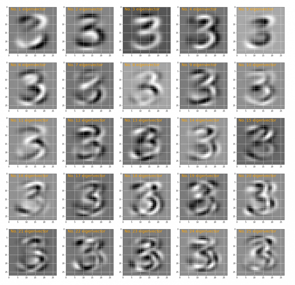
You have to keep it in mind that the data are all shown as 28 by 28 pixel grayscale images, but in the process of PCA, they are all processed as 28 * 28 = 784 dimensional vectors. After applying PCA on the 784 dimensional vectors of images of ‘3,’ the first 25 eigenvectors are as below. You can see that at the beginning the eigenvectors partly retain the shapes of ‘3,’ but they are distorted as the eigenvalues get smaller. We can guess that the latter eigenvalues are not that helpful in reconstructing the shape of ‘3.’

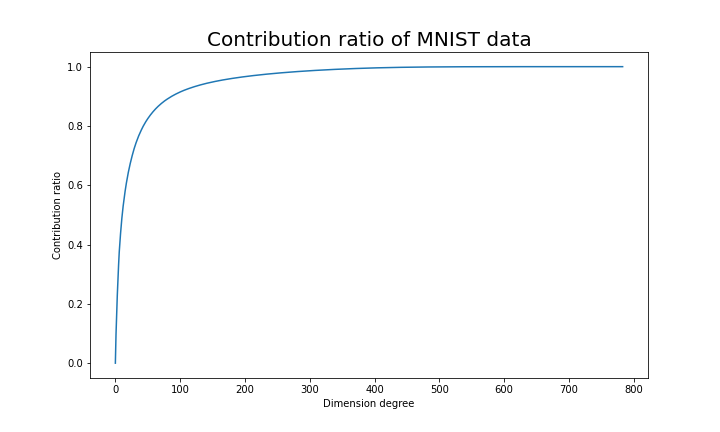
Just as we saw in the last section, you you can cut off axes of eigenvectors with small eigenvalues and reduce the dimension of MNIST data. The figure below shows how contribution ratio of MNIST data grows. You can see that around 200 dimension degree, the contribution ratio reaches around 0.95. Then we can guess that even if we reduce the dimension of MNIST from 784 to 200 we can retain the most of the structure of original data.

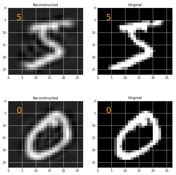
Some results of reconstruction of data from 200 dimensional space are as below. You can set how many images to display by adjusting NUMBER_OF_RESULTS in the code. And if you set LATENT_DIMENSION as 784, you can completely reconstruct the data.

* I make study materials on machine learning, sponsored by DATANOMIQ. I do my best to make my content as straightforward but as precise as possible. I include all of my reference sources. If you notice any mistakes in my materials, including grammatical errors, please let me know (email: yasuto.tamura@datanomiq.de). And if you have any advice for making my materials more understandable to learners, I would appreciate hearing it.

*I attatched the codes I used to make the figures in this article. You can just copy, paste, and run, sometimes installing necessary libraries.

import numpy as np

import keras # There should be some other simpler ways to download MNIST dataset,

# but at least on my laptop, this was the easiest.

import matplotlib.pyplot as plt

# Configuration part

USE_ALL_NUMBERS = False

WHICH_NUMBER = 3

W_RAW_DATA = 3

H_RAW_DATA = 1 # 1<= W_RAW_DATA*H_RAW_DATA <= 28*28

H_EIGENVECTORS = 5

W_EIGENVECTORS = 5 # 1<= H_EIGENVECTORS*W_EIGENVECTORS <= 28*28

# Preparing data

mnist = keras.datasets.mnist

(data, labels), (_, _) = mnist.load_data()

data = data.reshape([-1, 28*28])

if USE_ALL_NUMBERS:

data_to_use = data

labels_to_use = labels

else:

data_to_use = data[labels==WHICH_NUMBER]

labels_to_use = labels[labels==WHICH_NUMBER]

# Applying PCA to the data to use

ave = np.mean(data_to_use, axis=0)

covariance_matrix = np.dot((data_to_use - ave).T, (data_to_use - ave))

eigen_values, eigen_vectors = np.linalg.eig(covariance_matrix)

sorted_index = eigen_values.argsort()[::-1]

eigen_values=eigen_values[sorted_index]

eigen_vectors=eigen_vectors[:, sorted_index].real

plt.ﬁgure(1, ﬁgsize=(5*W_RAW_DATA, 5*H_RAW_DATA))

plt.gray()

for id in range(1*3):

plt.subplot(1, 3, id + 1)

img = data_to_use[id, :].reshape(28, 28)

plt.pcolor(img)

plt.text(1, 2, "No. %d raw data" % (id+1),

color='orange', fontsize=20)

plt.xlim(0, 27)

plt.ylim(27, 0)

plt.grid('on', color='white')

plt.savefig("MNIST_raw_data_3.png")

plt.show()

plt.ﬁgure(1, ﬁgsize=(W_EIGENVECTORS*5, H_EIGENVECTORS*5))

plt.gray()

for id in range(H_EIGENVECTORS*W_EIGENVECTORS):

plt.subplot(H_EIGENVECTORS, W_EIGENVECTORS, id + 1)

img = eigen_vectors.T[id, :].reshape(28, 28)

plt.pcolor(img)

plt.text(1, 2, "No. %d eigenvector" % (id+1),

color='orange', fontsize=20)

plt.xlim(0, 27)

plt.ylim(27, 0)

plt.grid('on', color='white')

plt.savefig("MNIST_PCA_eigenvectors.png")

plt.show()

import numpy as np

import keras

import matplotlib.pyplot as plt

# Configuration part

USE_ALL_NUMBERS = True

NUMBER_OF_RESULTS = 10

LATENT_DIMENSION = 95 # From 1 to 28*28=784

# Preparing data

mnist = keras.datasets.mnist

(data, labels), (_, _) = mnist.load_data()

data = data.reshape([-1, 28*28])

if USE_ALL_NUMBERS:

data_to_use = data

labels_to_use = labels

else:

data_to_use = data[labels==WHICH_NUMBER]

labels_to_use = labels[labels==WHICH_NUMBER]

# Applying PCA to the data to use

ave = np.mean(data_to_use, axis=0)

covariance_matrix = np.dot((data_to_use - ave).T, (data_to_use - ave))

eigen_values, eigen_vectors = np.linalg.eig(covariance_matrix)

sorted_index = eigen_values.argsort()[::-1]

eigen_values=eigen_values[sorted_index]

eigen_vectors=eigen_vectors[:, sorted_index].real

contribution_ratio = np.array([eigen_values[:i].sum()/eigen_values.sum() for i in range(len(eigen_values))])

plt.figure(1, figsize=(10, 6))

plt.title("Contribution ratio of MNIST data", fontsize=20)

plt.plot(np.arange(len(eigen_values)), contribution_ratio)

plt.xlabel('Dimension degree')

plt.ylabel('Contribution ratio')

plt.show()

U_reduced = eigen_vectors[:, :LATENT_DIMENSION]

data_transformed = np.dot(eigen_vectors.T, data_to_use.T).T

data_transformed_and_reduced = data_transformed[:, :LATENT_DIMENSION]

x_recomposed = np.dot(U_reduced, data_transformed_and_reduced.T).T

plt.ﬁgure(1, ﬁgsize=(2*5, NUMBER_OF_RESULTS*5))

plt.subplots_adjust(hspace=0.4)

plt.gray()

for id in range(NUMBER_OF_RESULTS*2):

plt.subplot(NUMBER_OF_RESULTS, 2, id + 1)

if(id % 2 == 0):

img = x_recomposed[id//2, :].reshape(28, 28)

plt.title("Reconstructed")

else:

img = data_to_use[id//2, :].reshape(28, 28)

plt.title("Original")

plt.pcolor(img)

plt.text(3, 5, "%d" % (labels_to_use[id//2]),

color='orange', fontsize=28)

plt.xlim(0, 27)

plt.ylim(27, 0)

plt.grid('on', color='white')

plt.show()

100

101

102

103

104

105

106

107

108

109

110

111

112

113

114

115

116

117

118

119

120

121

122

123

124

125

126

127

128

129

130

131

132

133

134

135

136

137

138

139

140

141

142

143

144

145

146

147

148

149

150

151

152

153

154

155

156

157

import numpy as np

import matplotlib.pyplot as plt

from mpl_toolkits.mplot3d.proj3d import proj_transform

from mpl_toolkits.mplot3d.axes3d import Axes3D

from matplotlib.text import Annotation

from matplotlib.patches import FancyArrowPatch

import matplotlib.patches as mpatches

class Annotation3D(Annotation):

def __init__(self, text, xyz, *args, **kwargs):

super().__init__(text, xy=(0,0), *args, **kwargs)

self._xyz = xyz

def draw(self, renderer):

x2, y2, z2 = proj_transform(*self._xyz, renderer.M)

self.xy=(x2,y2)

super().draw(renderer)

def _annotate3D(ax,text, xyz, *args, **kwargs):

'''Add anotation `text` to an `Axes3d` instance.'''

annotation= Annotation3D(text, xyz, *args, **kwargs)

ax.add_artist(annotation)

setattr(Axes3D,'annotate3D',_annotate3D)

class Arrow3D(FancyArrowPatch):

def __init__(self, x, y, z, dx, dy, dz, *args, **kwargs):

super().__init__((0,0), (0,0), *args, **kwargs)

self._xyz = (x,y,z)

self._dxdydz = (dx,dy,dz)

def draw(self, renderer):

x1,y1,z1 = self._xyz

dx,dy,dz = self._dxdydz

x2,y2,z2 = (x1+dx,y1+dy,z1+dz)

xs, ys, zs = proj_transform((x1,x2),(y1,y2),(z1,z2), renderer.M)

self.set_positions((xs[0],ys[0]),(xs[1],ys[1]))

super().draw(renderer)

def _arrow3D(ax, x, y, z, dx, dy, dz, *args, **kwargs):

'''Add an 3d arrow to an `Axes3D` instance.'''

arrow = Arrow3D(x, y, z, dx, dy, dz, *args, **kwargs)

ax.add_artist(arrow)

setattr(Axes3D,'arrow3D',_arrow3D)

jp_score = np.array([49, 58, 64, 65, 54, 58, 49, 67, 54, 66, 72, 66, 54, 64, 39,

56, 54, 56, 48, 57, 57, 47, 50, 60, 72, 54, 59, 61, 64, 70])

math_score = np.array([51, 58, 56, 70, 45, 70, 45, 69, 66, 73, 71, 72, 57, 53, 58,

57, 71, 63, 53, 62, 62, 59, 57, 65, 74, 66, 72, 50, 69, 60])

en_score = np.array([59, 63, 68, 77, 55, 71, 57, 79, 66, 81, 81, 77, 62, 67, 56,

62, 70, 67, 61, 70, 68, 59, 61, 71, 77, 66, 70, 59, 68, 71])

mean_vector = np.array([jp_score.mean(), math_score.mean(), en_score.mean()])

data_matrix = np.c_[jp_score, math_score, en_score]

data_mean_reduced = data_matrix - mean_vector

covariance_matrix = np.dot(data_mean_reduced.T, data_mean_reduced) / len(jp_score)

eigen_values, eigen_vectors = np.linalg.eig(covariance_matrix)

sorted_index = eigen_values.argsort()[::-1]

eigen_values=eigen_values[sorted_index]

eigen_vectors=eigen_vectors[:, sorted_index]

eigen_values, eigen_vectors = np.linalg.eig(covariance_matrix)

sorted_idx = eigen_values.argsort()[::-1]

eigen_values = eigen_values[sorted_idx]

eigen_vectors = eigen_vectors[:,sorted_idx]

eigen_vectors = eigen_vectors.astype(float)

subject_labels = ['Japanese score deviation', 'Math score deviation', 'English score deviation']

const_range = 2

X = np.arange(-const_range, const_range + 1, 1)

Y = np.arange(-const_range, const_range + 1, 1)

Z = np.arange(-const_range, const_range + 1, 1)

U_x, U_y, U_z = np.meshgrid(X, Y, Z)

V_x = np.zeros((len(U_x), len(U_y), len(U_z)))

V_y = np.zeros((len(U_x), len(U_y), len(U_z)))

V_z = np.zeros((len(U_x), len(U_y), len(U_z)))

temp_vec = np.zeros((1, 3))

W_x = np.zeros((len(U_x), len(U_y), len(U_z)))

W_y = np.zeros((len(U_x), len(U_y), len(U_z)))

W_z = np.zeros((len(U_x), len(U_y), len(U_z)))

fig = plt.figure(figsize=(15, 15))

grid_range = 15

for idx in range(2):

if idx ==0:

ax = fig.add_subplot(1, 2, idx + 1, projection='3d')

for i in range(len(U_x)):

for j in range(len(U_x)):

for k in range(len(U_x)):

temp_vec[0][0] = U_x[i][j][k]

temp_vec[0][1] = U_y[i][j][k]

temp_vec[0][2] = U_z[i][j][k]

temp_vec[0] = np.dot(covariance_matrix, temp_vec[0])

V_x[i][j][k] = temp_vec[0][0]

V_y[i][j][k] = temp_vec[0][1]

V_z[i][j][k] = temp_vec[0][2]

W_x[i][j][k] = (V_x[i][j][k] - U_x[i][j][k]) / (2*grid_range)

W_y[i][j][k] = (V_y[i][j][k] - U_y[i][j][k]) / (2*grid_range)

W_z[i][j][k] = (V_z[i][j][k] - U_z[i][j][k]) / (2*grid_range)

ax.arrow3D(0, 0, 0,

U_x[i][j][k], U_y[i][j][k], U_z[i][j][k],

mutation_scale=10, arrowstyle="-|>", fc='dimgrey', ec='dimgrey')

#ax.arrow3D(0, 0, 0,

# V_x[i][j][k], V_y[i][j][k], V_z[i][j][k],

# mutation_scale=10, arrowstyle="-|>", fc='red', ec='red')

ax.arrow3D(U_x[i][j][k], U_y[i][j][k], U_z[i][j][k],

W_x[i][j][k], W_y[i][j][k], W_z[i][j][k],

mutation_scale=10, arrowstyle="-|>", fc='darkviolet', ec='darkviolet')

if idx==1:

ax = fig.add_subplot(1, 2, idx + 1, projection='3d')

ax.scatter(data_mean_reduced[:, 0], data_mean_reduced[:, 1], data_mean_reduced[:, 2], marker='o', s=80)

ax.arrow3D(0, 0, 0, eigen_vectors.T[0][0]*10, eigen_vectors.T[0][1]*10, eigen_vectors.T[0][2]*10,

mutation_scale=10, arrowstyle="-|>", fc='orange', ec='orange', lw = 3)

ax.arrow3D(0, 0, 0, eigen_vectors.T[1][0]*10, eigen_vectors.T[1][1]*10, eigen_vectors.T[1][2]*10,

mutation_scale=10, arrowstyle="-|>", fc='orange', ec='orange', lw = 3)

ax.arrow3D(0, 0, 0, eigen_vectors.T[2][0]*10, eigen_vectors.T[2][1]*10, eigen_vectors.T[2][2]*10,

mutation_scale=10, arrowstyle="-|>", fc='orange', ec='orange', lw = 3)

ax.text(eigen_vectors.T[0][0]*8 , eigen_vectors.T[0][1]*8, eigen_vectors.T[0][2]*8+1, r'$u_1$', fontsize=20)

ax.text(eigen_vectors.T[1][0]*8 , eigen_vectors.T[1][1]*8, eigen_vectors.T[1][2]*8, r'$u_2$', fontsize=20)

ax.text(eigen_vectors.T[2][0]*8 , eigen_vectors.T[2][1]*8, eigen_vectors.T[2][2]*8, r'$u_3$', fontsize=20)

ax.set_xlim(-grid_range, grid_range)

ax.set_ylim(-grid_range, grid_range)

ax.set_zlim(-grid_range, grid_range)

#ax.set_xlabel(r'$x_1$', fontsize=25)

#ax.set_ylabel(r'$x_2$', fontsize=25)

#ax.set_zlabel(r'$x_3$', fontsize=25)

ax.set_xlabel(subject_labels[0], fontsize=10)

ax.set_ylabel(subject_labels[1], fontsize=10)

ax.set_zlabel(subject_labels[2], fontsize=10)

#lt.savefig("visualizing_covariance_matrix.png")

plt.show()

Rethinking linear algebra: visualizing linear transformations and eigenvectors

October 27, 2020/in Data Mining, Data Science, Machine Learning, Main Category, Mathematics/by Yasuto Tamura

In terms of calculation processes of Principal Component Analysis (PCA) or Linear Discriminant Analysis (LDA), which are the dimension reduction techniques I am going to explain in the following articles, diagonalization is what they are all about. Throughout this article, I would like you to have richer insight into diagonalization in order to prepare for understanding those basic dimension reduction techniques.

When our professor started a lecture on the last chapter of our textbook on linear algebra, he said “It is no exaggeration to say that everything we have studied is for this ‘diagonalization.'” Until then we had to write tons of numerical matrices and vectors all over our notebooks, calculating those products, adding their rows or columns to other rows or columns, sometimes transposing the matrices, calculating their determinants.

It was like the scene in “The Karate Kid,” where the protagonist finally understood the profound meaning behind the prolonged and boring “wax on, wax off” training given by Miyagi (or “jacket on, jacket off” training given by Jackie Chan). We had finally understood why we had been doing those seemingly endless calculations.

Source: http://thinkbedoleadership.com/secret-success-wax-wax-off/

But usually you can do those calculations easily with functions in the Numpy library. Unlike Japanese college freshmen, I bet you are too busy to reopen textbooks on linear algebra to refresh your mathematics. Thus I am going to provide less mathematical and more intuitive explanation of diagonalization in this article.

*This is the second article of the article series ” Illustrative introductions on dimension reduction .”

1, The mainstream ways of explaining diagonalization.

*The statements below are very rough for mathematical topics, but I am going to give priority to offering more visual understanding on linear algebra in this article. For further understanding, please refer to textbooks on linear algebra. If you would like to have minimum understandings on linear algebra needed for machine learning, I recommend the Appendix C of Pattern Recognition and Machine Learning by C. M. Bishop.

In most textbooks on linear algebra, the explanations on dioagonalization is like this (if you are not sure what diagonalization is or if you are allergic to mathematics, you do not have to read this seriously):

Let $V (dimV = D)$ be a vector space and let $T_A : V \rightarrow V$ be a mapping of $V$ into itself, defined as $T_A(v) = A \cdot \boldsymbol{v}$ , where $A$ is a $D\times D$ matrix and $\boldsymbol{v}$ is $D$ dimensional vector. An element $\boldsymbol{v} \in V$ is called an eigen vector if there exists a number $\lambda$ such that $A \cdot \boldsymbol{v}= \lambda \cdot \boldsymbol{v}$ and $\boldsymbol{v} \neq \boldsymbol{0}$ . In this case $\lambda$ is uniquely determined and is called an eigen value of $A$ belonging to the eigen vector $\boldsymbol{v}$ .

Any matrix $A$ has $D$ eigen values $\lambda_{i}$ , belonging to $\boldsymbol{v}_{i} (i=1, 2, …., D)$ . If $\boldsymbol{v}_{i}$ is basis of the vector space $V$ , then $A$ is diagonalizable.

When $A$ is diagonalizable, with $D \times D$ matrices $P = (\boldsymbol{v}_{1}, \dots, \boldsymbol{v}_{D})$ , whose column vectors are eigen vectors $\boldsymbol{v}_{i} (i=1, 2, …., D)$ , the following equation holds: $P^{-1}AP = \Lambda$ , where $\Lambda = diag(\lambda_{1}, \dots, \lambda_{D})= \begin{pmatrix} \lambda_{1} & 0& \ldots &0\\ 0 & \lambda_{2} & \ldots & 0 \\ \vdots & \vdots & \ddots & \vdots \\ 0 & 0 & \ldots & \lambda_{D} \end{pmatrix}$ .

And when $A$ is diagonalizable, you can diagonalize $A$ as below.

Most textbooks keep explaining these type of stuff, but I have to say they lack efforts to make it understandable to readers with low mathematical literacy like me. Especially if you have to apply the idea to data science field, I believe you need more visual understanding of diagonalization. Therefore instead of just explaining the definitions and theorems, I would like to take a different approach. But in order to understand them in more intuitive ways, we first have to rethink waht linear transformation $T_A$ means in more visible ways.

2, Linear transformations

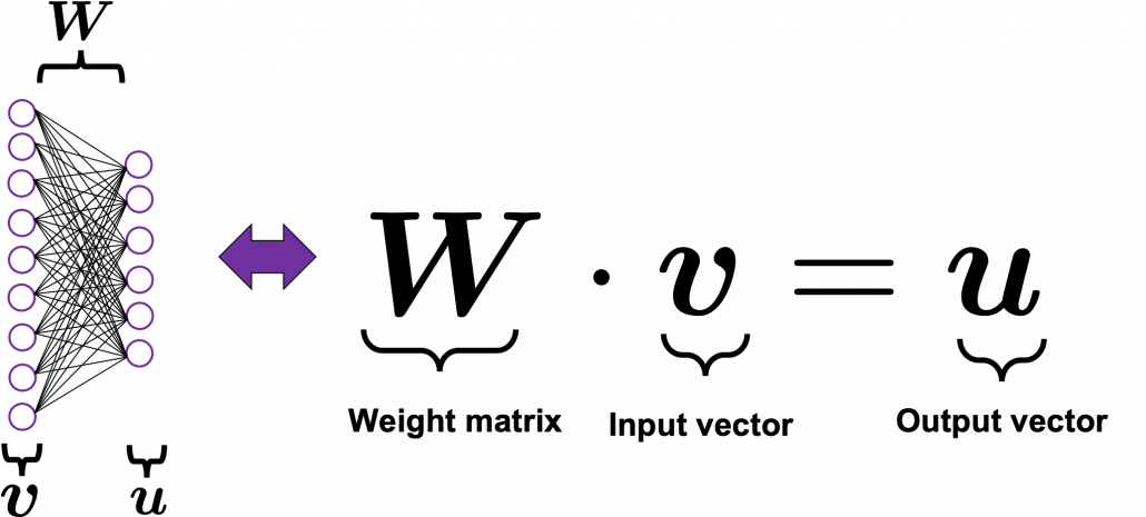
Even though I did my best to make this article understandable to people with little prerequisite knowledge, you at least have to understand linear transformation of numerical vectors and with matrices. Linear transformation is nothing difficult, and in this article I am going to use only 2 or 3 dimensional numerical vectors or square matrices. You can calculate linear transformation of $\boldsymbol{v}$ by $A$ as equations in the figure. In other words, $\boldsymbol{u}$ is a vector transformed by $A$ .

*I am not going to use the term “linear transformation” in a precise way in the context of linear algebra. In this article or in the context of data science or machine learning, “linear transformation” for the most part means products of matrices or vectors.

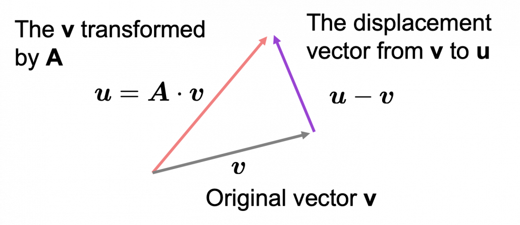
*Forward/back propagation of deep learning is mainly composed of this linear transformation. You keep linearly transforming input vectors, frequently transforming them with activation functions, which are for the most part not linear transformation.

As you can see in the equations above, linear transformation with $A$ transforms a vector to another vector. Assume that you have an original vector $\boldsymbol{v}$ in grey and that the vector $\boldsymbol{u}$ in pink is the transformed $\boldsymbol{v}$ by $A$ is. If you subtract $\boldsymbol{v}$ from $\boldsymbol{u}$ , you can get a displacement vector, which I displayed in purple. A displacement vector means the transition from a vector to another vector.

Let’s calculate the displacement vector with more vectors $\boldsymbol{v}$ . Assume that $A =\begin{pmatrix} 3 & 1 \\ 1 & 2 \end{pmatrix}$ , and I prepared several grid vectors $\boldsymbol{v}$ in grey as you can see in the figure below. If you transform those grey grid points with $A$ , they are mapped into the vectors $\boldsymbol{u}$ in pink. With those vectors in grey or pink, you can calculate the their displacement vectors $\boldsymbol{u} - \boldsymbol{v}$ , which are in purple.

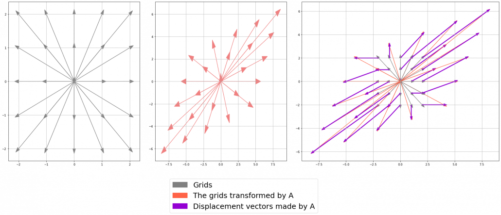
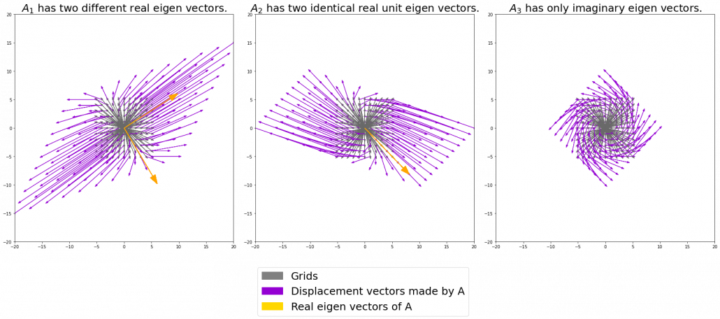
The displacement vectors in the figure above have some tendencies. In order to see that more clearly, let’s calculate displacement vectors with several matrices $A$ and more grid points. Assume that you have three $2 \times 2$ square matrices $A_1 =\begin{pmatrix} 3 & 1 \\ 1 & 2 \end{pmatrix}, A_2 =\begin{pmatrix} 3 & 1 \\ -1 & 1 \end{pmatrix}, A_3 =\begin{pmatrix} 1 & -1 \\ 1 & 1 \end{pmatrix}$ , and I plotted displace vectors made by the matrices respectively in the figure below.

I think you noticed some characteristics of the displacement vectors made by those linear transformations: the vectors are swirling and many of them seem to be oriented in certain directions. To be exact, some displacement vectors extend in the same directions as some of original vectors in grey. That means linear transformation by $A$ did not change the direction of the original vector $\boldsymbol{v}$ , and the unchanged vectors are called eigen vectors. Real eigen vectors of each A are displayed as arrows in yellow in the figure above. But when it comes to $A_3$ , the matrix does not have any real eigan values.

In linear algebra, depending on the type matrices $A$ , you have to consider various cases such as whether the matrices have real or imaginary eigen values, whether the matrices are diagonalizable, whether the eigen vectors are orthogonal, or whether they are unit vectors. But those topics are out of the scope of this article series, so please refer to textbooks on linear algebra if you are interested.

Luckily, however, in terms of PCA or LDA, you only have to consider a type of matrices named positive semidefinite matrices, which $A_1$ is classified to, and I am going to explain positive semidefinite matrices in the fourth section.

3, Eigen vectors as coordinate system

Source: Ian Stewart, “Professor Stewart’s Cabinet of Mathematical Curiosities,” (2008), Basic Books

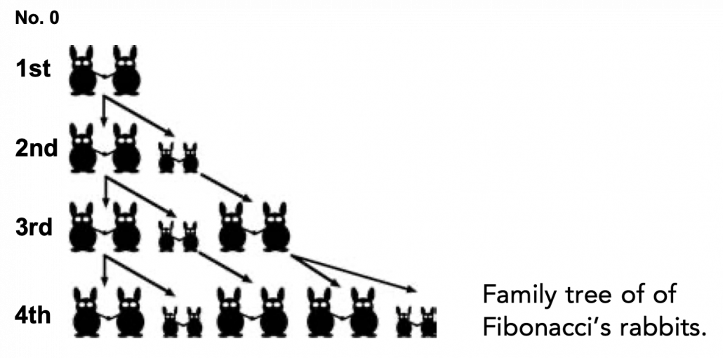
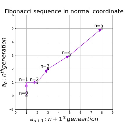
Let me take Fibonacci numbers as an example to briefly see why diagonalization is useful. Fibonacci is sequence is quite simple and it is often explained using an example of pairs of rabbits increasing generation by generation. Let $a_n (n=0, 1, 2, …)$ be the number of pairs of grown up rabbits in the $n^{th}$ generation. One pair of grown up rabbits produce one pair of young rabbit The concrete values of $a_n$ are $a_0 = 0$ , $a_1 = 1$ , $a_2=1$ , $a_3=2$ , $a_4=3$ , $a_5=5$ , $a_6=8$ , $a_7=13, \dots$ . Assume that $A =\begin{pmatrix} 1 & 1 \\ 1 & 0 \end{pmatrix}$ and that $\begin{pmatrix} a_1 \\ a_0 \end{pmatrix} =\begin{pmatrix} 1 \\ 0 \end{pmatrix}$ , then you can calculate the number of the pairs of grown up rabbits in the next generation with the following recurrence relation. $\begin{pmatrix} a_{n+1} \\ a_{n} \end{pmatrix}=\begin{pmatrix} 1 & 1 \\ 1 & 0 \end{pmatrix} \cdot \begin{pmatrix} a_{n+1} \\ a_{n} \end{pmatrix}$ .Let $\boldsymbol{a}_n$ be $\begin{pmatrix} a_{n+1} \\ a_{n} \end{pmatrix}$ , then the recurrence relation can be written as $\boldsymbol{a}_{n+1} = A \boldsymbol{a}_n$ , and the transition of $\boldsymbol{a}_n$ are like purple arrows in the figure below. It seems that the changes of the purple arrows are irregular if you look at the plots in normal coordinate.

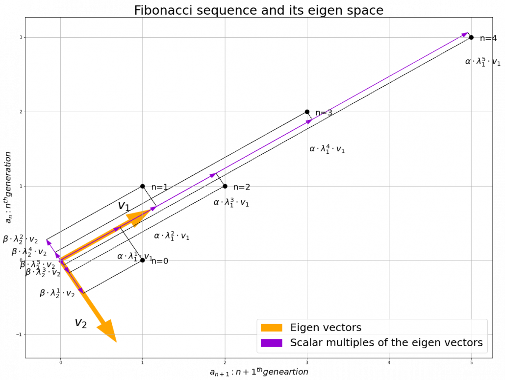
Assume that $\lambda _1, \lambda_2 (\lambda _1< \lambda_2)$ are eigen values of $A$ , and $\boldsymbol{v}_1, \boldsymbol{v}_2$ are eigen vectors belonging to them respectively. Also let $\alpha, \beta$ scalars such that $\begin{pmatrix} a_{1} \\ a_{0} \end{pmatrix} = \begin{pmatrix} 1 \\ 0 \end{pmatrix} = \alpha \boldsymbol{v}_1 + \beta \boldsymbol{v}_2$ . According to the definition of eigen values and eigen vectors belonging to them, the following two equations hold: $A\boldsymbol{v}_1 = \lambda_1 \boldsymbol{v}_1, A\boldsymbol{v}_2 = \lambda_2 \boldsymbol{v}_2$ . If you calculate $\boldsymbol{a}_1$ is, using eigen vectors of $A$ , $\boldsymbol{a}_1 = A\boldsymbol{a}_0 = A (\alpha \boldsymbol{v}_1 + \beta \boldsymbol{v}_2) = \alpha\lambda _1 \boldsymbol{v}_1 + \beta \lambda_2 \boldsymbol{v}_2$ . In the same way, $\boldsymbol{a}_2 = A\boldsymbol{a}_1 = A (\alpha\lambda _1 \boldsymbol{v}_1 + \beta \lambda_2 \boldsymbol{v}_2) = \alpha\lambda _{1}^{2} \boldsymbol{v}_1 + \beta \lambda_{2}^{2} \boldsymbol{v}_2$ , and $\boldsymbol{a}_3 = A\boldsymbol{a}_2 = A (\alpha\lambda _{1}^{2} \boldsymbol{v}_1 + \beta \lambda_{2}^{2} \boldsymbol{v}_2) = \alpha\lambda _{1}^{3} \boldsymbol{v}_1 + \beta \lambda_{2}^{3} \boldsymbol{v}_2$ . These equations show that in coordinate system made by eigen vectors of $A$ , linear transformation by $A$ is easily done by just multiplying eigen values with each eigen vector. Compared to the graph of Fibonacci numbers above, in the figure below you can see that in coordinate system made by eigen vectors the plots changes more systematically generation by generation.

In coordinate system made by eigen vectors of square matrices, the linear transformations by the matrices can be much more straightforward, and this is one powerful strength of eigen vectors.

*I do not major in mathematics, so I am not 100% sure, but vectors in linear algebra have more abstract meanings. Various things in mathematics can be vectors, even though in machine learning or data science we mainly use numerical vectors with more concrete elements. We can also say that matrices are a kind of maps. That is just like, at least in my impression, even though a real town is composed of various components such as houses, smooth or bumpy roads, you can simplify its structure with simple orthogonal lines, like the map of Manhattan. But if you know what the town actually looks like, you do not have to follow the zigzag path on the map.

4, Eigen vectors of positive semidefinite matrices

In the second section of this article I told you that, even though you have to consider various elements when you discuss general diagonalization, in terms of PCA and LDA we mainly use only a type of matrices named positive semidefinite matrices. Let $A$ be a $D \times D$ square matrix. If $\boldsymbol{x}^T A \boldsymbol{x} \geq 0$ for all values of the vector $\boldsymbol{x}$ , the $A$ is said to be a positive semidefinite matrix. And also it is known that $A$ being a semidefinite matrix is equivalent to $\lambda _{i} \geq 0$ for all the eigen values $\lambda_i (i=1, \dots , D)$ .

*I think most people first learn a type of matrices called positive definite matrices. Let $A$ be a $D \times D$ square matrix. If $\boldsymbol{x}^T A \boldsymbol{x} > 0$ for all values of the vector $\boldsymbol{x}$ , the $A$ is said to be a positive definite matrix. You have to keep it in mind that even if all the elements of $A$ are positive, $A$ is not necessarly positive definite/semidefinite.

Just as we did in the second section of this article, let’s visualize displacement vectors made by linear transformation with a $3 \times 3$ square positive semidefinite matrix $A$ .

*In fact $A_1 =\begin{pmatrix} 3 & 1 \\ 1 & 2 \end{pmatrix}$ , whose linear transformation I visualized the second section, is also positive semidefinite.

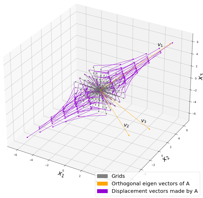
Let’s visualize linear transformations by a positive definite matrix $A = \frac{1}{50} \begin{pmatrix} 60.45 & 33.63 & 46.29 \\33.63 & 68.49 & 50.93 \\ 46.29 & 50.93 & 53.61 \end{pmatrix}$ . I visualized the displacement vectors made by the $A$ just as the same way as in the second section of this article. The result is as below, and you can see that, as well as the displacement vectors made by $A_1$ , the three dimensional displacement vectors below are swirling and extending in three directions, in the directions of the three orthogonal eigen vectors $\boldsymbol{v}_1, \boldsymbol{v}_2$ , and $\boldsymbol{v}_3$ .

*It might seem like a weird choice of a matrix, but you are going to see why I chose it in the next article.

You might have already noticed $A_1 =\begin{pmatrix} 3 & 1 \\ 1 & 2 \end{pmatrix}$ and $A = \frac{1}{50} \begin{pmatrix} 60.45 & 33.63 & 46.29 \\33.63 & 68.49 & 50.93 \\ 46.29 & 50.93 & 53.61 \end{pmatrix}$ are both symmetric matrices and that their elements are all real values, and that their diagonal elements are all positive values. Super importantly, when all the elements of a $D \times D$ symmetric matrix $A$ are real values and its eigen values are $\lambda_{i} (i=1, \dots , D)$ , there exist orthonormal matrices $U$ such that $U^{-1}AU = \Lambda$ , where $\Lambda = diag(\lambda_{1}, \dots , \lambda_{D})$ .

*The title of this section might be misleading, but please keep it in mind that positive definite/semidefinite matrices are not necessarily real symmetric matrices. And real symmetric vectors are not necessarily positive definite/semidefinite matrices.

5, Orthonormal matrices and rotation of vectors

In this section I am gong to explain orthonormal matrices, as known as rotation matrices. If a $D\times D$ matrix $U$ is an orthonormal matrix, column vectors of $U$ are orthonormal, which means $U = (\boldsymbol{u}_1 \dots \boldsymbol{u}_D)$ , where $\begin{cases} \boldsymbol{u}_{i}^{T}\boldsymbol{u}_{j} = 1 \quad (i = j) \\ \boldsymbol{u}_{i}^{T}\boldsymbol{u}_{j} = 0 \quad (i\neq j) \end{cases}$ . In other words column vectors $\boldsymbol{u}_{i}$ form an orthonormal coordinate system.

Orthonormal matrices $U$ have several important properties, and one of the most important properties is $U^{-1} = U^{T}$ . Combining this fact with what I have told you so far, you we can reach one conclusion: you can orthogonalize a real symmetric matrix $A$ as $U^{T}AU = \Lambda$ . This is known as spectral decomposition or singular value decomposition.

Another important property of $U$ is that $U^{T}$ is also orthonormal. In other words, assume $U$ is orthonormal and that $U = (\boldsymbol{u}_1 \dots \boldsymbol{u}_D) = \begin{pmatrix} -\boldsymbol{v_1}^{T}- \\ \vdots \\ -\boldsymbol{v_D}^{T}- \end{pmatrix}$ , $(\boldsymbol{v}_1 \dots \boldsymbol{v}_D)$ also forms a orthonormal coordinate system.

…It seems things are getting too mathematical and abstract (for me), thus for now I am going to wrap up what I have explained in this article .

We have seen

Numerical matrices linearly transform vectors.
Certain linear transformations do not change the direction of vectors in certain directions, which are called eigen vectors.
Making use of eigen vectors, you can form new coordinate system which can describe the linear transformations in a more straightforward way.
You can diagonalize a real symmetric matrix $A$ with an orthonormal matrix $U$ .

Of our current interest is what kind of linear transformation the real symmetric positive definite matrix enables. I am going to explain why the purple vectors in the figure above is swirling in the upcoming articles. Before that, however, we are going to see one application of what we have seen in this article, on dimension reduction. To be concrete the next article is going to be about principal component analysis (PCA), which is very important in many fields.

*In short, the orthonormal matrix $U$ , which I mentioned above enables rotation of matrix, and the diagonal matrix $diag(\lambda_1, \dots, \lambda_D)$ expands or contracts vectors along each axis. I am going to explain that more precisely in the upcoming articles.

*I attatched the codes I used to make the figures in this article. You can just copy, paste, and run, sometimes installing necessary libraries.

import matplotlib.pyplot as plt

import numpy as np

import matplotlib.patches as mpatches

T_A = np.array([[1, 1],

[1, 0]])

total_step = 5

x = np.zeros((total_step, 2))

x[0] = np.array([1, 0])

for i in range(total_step - 1):

x[i + 1] = np.dot(T_A, x[i])

eigen_values, eigen_vectors = np.linalg.eig(T_A)

idx = eigen_values.argsort()[::-1]

eigen_values = eigen_values[idx]

eigen_vectors = eigen_vectors[:,idx]

for i in range(len(eigen_vectors)):

if(eigen_vectors.T[i][0] < 0):

eigen_vectors.T[i] = - eigen_vectors.T[i]

v_initial = x[0]

v_coefficients = np.zeros((total_step , 2))

v_coefficients[0] = np.dot(v_initial , np.linalg.inv(eigen_vectors.T))

for i in range(total_step-1):

v_coefficients[i + 1] = v_coefficients[i] * eigen_values

v_1_list = np.zeros((total_step + 1, 2))

v_2_list = np.zeros((total_step + 1, 2))

for i in range(total_step):

v_1_list[i+1] = v_coefficients.T[0][i]*eigen_vectors.T[0]

v_2_list[i+1] = v_coefficients.T[1][i]*eigen_vectors.T[1]

plt.figure(figsize=(20, 15))

fontsize = 20

small_shift = 0.2

plt.plot(x[:, 0], x[:, 1], marker='o', linestyle='none', markersize=10, color='black')

plt.arrow(0, 0, eigen_vectors.T[0][0], eigen_vectors.T[0][1], width=0.05, head_width=0.2, color='orange')

plt.arrow(0, 0, eigen_vectors.T[1][0], eigen_vectors.T[1][1], width=0.05, head_width=0.2, color='orange')

plt.text(eigen_vectors.T[0][0], eigen_vectors.T[0][1]+small_shift, r'$v_{1}$', va='center',ha='right', fontsize=fontsize + 10)

plt.text(eigen_vectors.T[1][0] - small_shift, eigen_vectors.T[1][1],r'$v_{2}$', va='center',ha='right', fontsize=fontsize + 10)

for i in range(total_step):

plt.arrow(0, 0, v_1_list[i+1][0], v_1_list[i+1][1], head_width=0.05, color='darkviolet', length_includes_head=True)

plt.arrow(0, 0, v_2_list[i+1][0], v_2_list[i+1][1], head_width=0.05, color='darkviolet', length_includes_head=True)

plt.text(v_1_list[i+1][0] + 2*small_shift , v_1_list[i+1][1]-2*small_shift,r'$\alpha \cdot \lambda_{0} ^{1} \cdot v_{2} $'.format(1,i+1, 1),va='center',ha='right', fontsize=fontsize)

plt.text(v_2_list[i+1][0]-0.1, v_2_list[i+1][1],r'$\beta \cdot \lambda_{0} ^{1} \cdot v_{2} $'.format(2, i+1, 2),va='center',ha='right', fontsize=fontsize)

plt.arrow(v_1_list[i+1][0], v_1_list[i+1][1], v_2_list[i+1][0], v_2_list[i+1][1], head_width=0, color='black', linestyle='--', length_includes_head=True)

plt.arrow(v_2_list[i+1][0], v_2_list[i+1][1], v_1_list[i+1][0], v_1_list[i+1][1], head_width=0, color='black', linestyle='--', length_includes_head=True)

orange_patch = mpatches.Patch(color='orange', label='Eigen vectors')

purple_patch = mpatches.Patch(color='darkviolet', label='Scalar multiples of the eigen vectors')

plt.legend(handles=[orange_patch, purple_patch], fontsize=25, loc='lower right')

for i in range(total_step):

plt.text(x[i][0]+0.1, x[i][1]-0.05, r'n={0}'.format(i), fontsize=20)

plt.grid(True)

plt.ylabel("$a_{n}: n^{th} generation$", fontsize=20)

plt.xlabel("$a_{n+1}: n+1 ^{th} geneartion$", fontsize=20)

plt.title("Fibonacci sequence and its eigen space", fontsize=30)

#plt.savefig("Fibonacci_eigen_space.png")

plt.show()

import matplotlib.pyplot as plt

import numpy as np

import matplotlib.patches as mpatches

const_range = 10

X = np.arange(-const_range, const_range + 1, 1)

Y = np.arange(-const_range, const_range + 1, 1)

U_x, U_y = np.meshgrid(X, Y)

T_A_0 = np.array([[3, 1],

[1, 2]])

T_A_1 = np.array([[3, 1],

[-1, 1]])

T_A_2 = np.array([[1, -1],

[1, 1]])

T_A_list = np.array((T_A_0, T_A_1, T_A_2))

const_range = 5

plt.figure(figsize=(30, 10))

plt.subplots_adjust(wspace=0.1)

labels = ["Grids", "Displacement vectors made by A", "Real eigen vectors of A"]

title_list = [r"$A_1$ has two different real eigen vectors.", r"$A_2$ has two identical real unit eigen vectors.", r"$A_3$ has only imaginary eigen vectors."]

for idx in range(len(T_A_list)):

eigen_values, eigen_vectors = np.linalg.eig(T_A_list[idx])

sorted_idx = eigen_values.argsort()[::-1]

eigen_values = eigen_values[sorted_idx]

eigen_vectors = eigen_vectors[:,sorted_idx]

eigen_vectors = eigen_vectors.astype(float)

for i in range(len(eigen_vectors)):

if(eigen_vectors.T[i][0] < 0):

eigen_vectors.T[i] = - eigen_vectors.T[i]

X = np.arange(-const_range, const_range + 1, 1)

Y = np.arange(-const_range, const_range + 1, 1)

U_x, U_y = np.meshgrid(X, Y)

V_x = np.zeros((len(U_x), len(U_y)))

V_y = np.zeros((len(U_x), len(U_y)))

temp_vec = np.zeros((1, 2))

W_x = np.zeros((len(U_x), len(U_y)))

W_y = np.zeros((len(U_x), len(U_y)))

plt.subplot(1, 3, idx + 1)

for i in range(len(U_x)):

for j in range(len(U_y)):

temp_vec[0][0] = U_x[i][j]

temp_vec[0][1] = U_y[i][j]

temp_vec[0] = np.dot(T_A_list[idx], temp_vec[0])

V_x[i][j] = temp_vec[0][0]

V_y[i][j] = temp_vec[0][1]

W_x[i][j] = V_x[i][j] - U_x[i][j]

W_y[i][j] = V_y[i][j] - U_y[i][j]

#plt.arrow(0, 0, V_x[i][j], V_y[i][j], head_width=0.1, color='red')

plt.arrow(0, 0, U_x[i][j], U_y[i][j], head_width=0.3, color='dimgrey', label=labels[0])

plt.arrow(U_x[i][j], U_y[i][j], W_x[i][j], W_y[i][j], head_width=0.3, color='darkviolet', label=labels[1])

range_const = 20

plt.xlim([-range_const, range_const])

plt.ylim([-range_const, range_const])

plt.title(title_list[idx], fontsize=25)

if idx==2:

continue

plt.arrow(0, 0, eigen_vectors.T[0][0]*10, eigen_vectors.T[0][1]*10, head_width=1, color='orange', label=labels[2])

plt.arrow(0, 0, eigen_vectors.T[1][0]*10, eigen_vectors.T[1][1]*10, head_width=1, color='orange', label=labels[2])

grey_patch = mpatches.Patch(color='grey', label='Grids')

purple_patch = mpatches.Patch(color='darkviolet', label='Displacement vectors made by A')

yellow_patch = mpatches.Patch(color='gold', label='Real eigen vectors of A')

plt.legend(handles=[grey_patch, purple_patch, yellow_patch], fontsize=25, loc='lower right', bbox_to_anchor=(-0.1, -.35))

#plt.savefig("linear_transformation.png")

plt.show()

100

101

102

103

104

105

106

107

108

109

110

111

112

113

114

115

116

117

118

119

120

121

122

123

124

125

126

127

128

129

130

131

132

133

134

135

136

137

138

139

140

141

142

143

144

145

146

147

148

# I borrowed codes from https://gist.github.com/WetHat/1d6cd0f7309535311a539b42cccca89c to make 3D arrows with matlotlib

import numpy as np

import matplotlib.pyplot as plt

from mpl_toolkits.mplot3d.proj3d import proj_transform

from mpl_toolkits.mplot3d.axes3d import Axes3D

from matplotlib.text import Annotation

from matplotlib.patches import FancyArrowPatch

import matplotlib.patches as mpatches

class Annotation3D(Annotation):

def __init__(self, text, xyz, *args, **kwargs):

super().__init__(text, xy=(0,0), *args, **kwargs)

self._xyz = xyz

def draw(self, renderer):

x2, y2, z2 = proj_transform(*self._xyz, renderer.M)

self.xy=(x2,y2)

super().draw(renderer)

def _annotate3D(ax,text, xyz, *args, **kwargs):

'''Add anotation `text` to an `Axes3d` instance.'''

annotation= Annotation3D(text, xyz, *args, **kwargs)

ax.add_artist(annotation)

setattr(Axes3D,'annotate3D',_annotate3D)

class Arrow3D(FancyArrowPatch):

def __init__(self, x, y, z, dx, dy, dz, *args, **kwargs):

super().__init__((0,0), (0,0), *args, **kwargs)

self._xyz = (x,y,z)

self._dxdydz = (dx,dy,dz)

def draw(self, renderer):

x1,y1,z1 = self._xyz

dx,dy,dz = self._dxdydz

x2,y2,z2 = (x1+dx,y1+dy,z1+dz)

xs, ys, zs = proj_transform((x1,x2),(y1,y2),(z1,z2), renderer.M)

self.set_positions((xs[0],ys[0]),(xs[1],ys[1]))

super().draw(renderer)

def _arrow3D(ax, x, y, z, dx, dy, dz, *args, **kwargs):

'''Add an 3d arrow to an `Axes3D` instance.'''

arrow = Arrow3D(x, y, z, dx, dy, dz, *args, **kwargs)

ax.add_artist(arrow)

setattr(Axes3D,'arrow3D',_arrow3D)

T_A = np.array([[60.45, 33.63, 46.29],

[33.63, 68.49, 50.93],

[46.29, 50.93, 53.61]])

T_A = T_A/50

const_range = 2

X = np.arange(-const_range, const_range + 1, 1)

Y = np.arange(-const_range, const_range + 1, 1)

Z = np.arange(-const_range, const_range + 1, 1)

U_x, U_y, U_z = np.meshgrid(X, Y, Z)

V_x = np.zeros((len(U_x), len(U_y), len(U_z)))

V_y = np.zeros((len(U_x), len(U_y), len(U_z)))

V_z = np.zeros((len(U_x), len(U_y), len(U_z)))

temp_vec = np.zeros((1, 3))

W_x = np.zeros((len(U_x), len(U_y), len(U_z)))

W_y = np.zeros((len(U_x), len(U_y), len(U_z)))

W_z = np.zeros((len(U_x), len(U_y), len(U_z)))

eigen_values, eigen_vectors = np.linalg.eig(T_A)

sorted_idx = eigen_values.argsort()[::-1]

eigen_values = eigen_values[sorted_idx]

eigen_vectors = eigen_vectors[:,sorted_idx]

eigen_vectors = eigen_vectors.astype(float)

fig = plt.figure(figsize=(15, 15))

ax = fig.add_subplot(111, projection='3d')

grid_range = const_range + 5

ax.set_xlim(-grid_range, grid_range)

ax.set_ylim(-grid_range, grid_range)

ax.set_zlim(-grid_range, grid_range)

eigen_values, eigen_vectors = np.linalg.eig(T_A)

sorted_idx = eigen_values.argsort()[::-1]

eigen_values = eigen_values[sorted_idx]

eigen_vectors = eigen_vectors[:,sorted_idx]

eigen_vectors = eigen_vectors.astype(float)

for i in range(len(eigen_vectors)):

if(eigen_vectors.T[i][0] < 0):

eigen_vectors.T[i] = - eigen_vectors.T[i]

for i in range(len(U_x)):

for j in range(len(U_x)):

for k in range(len(U_x)):

temp_vec[0][0] = U_x[i][j][k]

temp_vec[0][1] = U_y[i][j][k]

temp_vec[0][2] = U_z[i][j][k]

temp_vec[0] = np.dot(T_A, temp_vec[0])

V_x[i][j][k] = temp_vec[0][0]

V_y[i][j][k] = temp_vec[0][1]

V_z[i][j][k] = temp_vec[0][2]

W_x[i][j][k] = V_x[i][j][k] - U_x[i][j][k]

W_y[i][j][k] = V_y[i][j][k] - U_y[i][j][k]

W_z[i][j][k] = V_z[i][j][k] - U_z[i][j][k]

ax.arrow3D(0, 0, 0,

U_x[i][j][k], U_y[i][j][k], U_z[i][j][k],

mutation_scale=10, arrowstyle="-|>", fc='dimgrey', ec='dimgrey')

#ax.arrow3D(0, 0, 0,

# V_x[i][j][k], V_y[i][j][k], V_z[i][j][k],

# mutation_scale=10, arrowstyle="-|>", fc='red', ec='red')

ax.arrow3D(U_x[i][j][k], U_y[i][j][k], U_z[i][j][k],

W_x[i][j][k], W_y[i][j][k], W_z[i][j][k],

mutation_scale=10, arrowstyle="-|>", fc='darkviolet', ec='darkviolet')

ax.arrow3D(0, 0, 0, eigen_vectors.T[0][0]*10, eigen_vectors.T[0][1]*10, eigen_vectors.T[0][2]*10,

mutation_scale=10, arrowstyle="-|>", fc='orange', ec='orange')

ax.arrow3D(0, 0, 0, eigen_vectors.T[1][0]*10, eigen_vectors.T[1][1]*10, eigen_vectors.T[1][2]*10,

mutation_scale=10, arrowstyle="-|>", fc='orange', ec='orange')

ax.arrow3D(0, 0, 0, eigen_vectors.T[2][0]*10, eigen_vectors.T[2][1]*10, eigen_vectors.T[2][2]*10,

mutation_scale=10, arrowstyle="-|>", fc='orange', ec='orange')

ax.text(eigen_vectors.T[0][0]*8 , eigen_vectors.T[0][1]*8, eigen_vectors.T[0][2]*8+1, r'$v_1$', fontsize=20)

ax.text(eigen_vectors.T[1][0]*8 , eigen_vectors.T[1][1]*8, eigen_vectors.T[1][2]*8, r'$v_2$', fontsize=20)

ax.text(eigen_vectors.T[2][0]*8 , eigen_vectors.T[2][1]*8, eigen_vectors.T[2][2]*8, r'$v_3$', fontsize=20)

grey_patch = mpatches.Patch(color='grey', label='Grids')

orange_patch = mpatches.Patch(color='orange', label='Orthogonal eigen vectors of A')

purple_patch = mpatches.Patch(color='darkviolet', label='Displacement vectors made by A')

plt.legend(handles=[grey_patch, orange_patch, purple_patch], fontsize=20, loc='lower right')

ax.set_xlabel(r'$x_1$', fontsize=25)

ax.set_ylabel(r'$x_2$', fontsize=25)

ax.set_zlabel(r'$x_3$', fontsize=25)

#plt.savefig("symmetric_positive_definite_visualizaiton.png")

plt.show()

K Nearest Neighbour For Supervised Learning

October 10, 2020/in Artificial Intelligence, Data Science, Machine Learning, Main Category, Mathematics/by Ram Tavva

K-Nearest Neighbour (KNN) Algorithms is an easy-to-implement & advanced level supervised machine learning algorithm used for both – classification as well as regression problems. However, you can see a wide of its applications in classification problems across various industries.

If you’ve been shopping a lot in e-commerce sites like Amazon, Flipkart, Myntra, or love watching web series over Netflix and Amazon Prime, one common thing you’ve always noticed, and that is recommendations.

Are you wondering how they recommend you following your choice? They use KNN Supervised Learning to find out what you may need the next when you’re buying and recommend you with a few more products.

Imagine you’re looking for an iPhone to purchase. When you scroll down a little, you see some iPhone cases, tempered glasses – saying, “People who purchased an iPhone have also purchased these items. The same applies to Netflix and Amazon Prime. When you finished a show or a series, they give you recommendations of the same genre. And do it all using KNN supervised learning and classify the items for the best user experience.

Advantages Of KNN

Quickest Calculation Time
Simple Algorithms
High Accuracy
Versatile – best use for Regression and Classification.
Doesn’t make any assumptions about data.

Where KNN Are Mostly Used

Simple Recommendation Models
Image Recognition Technology
Decision-Making Models
Calculating Credit Rating

Choosing The Right Value For K

To choose the right value of K, you have to run KNN algorithms several times with different values of K and select the value of K, which reduces the number of errors you’ve come across and come out as the most stable value for K.

Your Step-By-Step Guide For Choosing The Value Of K

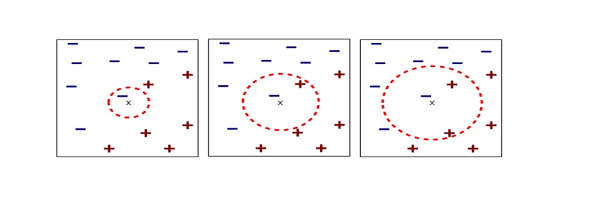
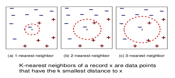
As you decrease the value of K to 1 (K = 1), you’ll reach a query point, where you get to see many elements from class A (-) and class B (+) where (-) is the only nearest neighbor. Reasonably, you would think about the query point to be most likely the red one. As K =1, which has a blue color, KNN incorrectly predicts the wrong color blue.
As you increase the value of K to 2 (K=2), you get to see two elements, (-) and (+) are the only nearest neighbor. As you have two values, which are of Class A and Class B, KNN incorrectly predicts the wrong values (Blue and Red).
As you increase the value of K to 3 (K=3), you get to see three elements (-) and (+), (+) are the only nearest neighbor. And this time, you got three values, one from blue and two from red. As your assumption is red, KNN correctly predicts the right value (Blue and Red, Red). Your answer is more stable this time compared to previous ones.

Conclusion

KNN works by finding the nearest distance between a query and all the elements in the database. By choosing the value for K, we get the closest to the query. And then, KNN algorithms look for the most frequent labels in classification and averages of labels in regression.

Illustrative introductions on dimension reduction

October 2, 2020/in Artificial Intelligence, Data Mining, Data Science, Machine Learning, Main Category, Mathematics/by Yasuto Tamura

“What is your image on dimensions?”

….That might be a cheesy question to ask to reader of Data Science Blog, but most people, with no scientific background, would answer “One dimension is a line, and two dimension is a plain, and we live in three-dimensional world.” After that if you ask “How about the fourth dimension?” many people would answer “Time?”

You can find books or writings about dimensions in various field. And you can use the word “dimension” in normal conversations, in many contexts.

*In Japanese, if you say “He likes two dimension.” that means he prefers anime characters to real women, as is often the case with Japanese computer science students.

The meanings of “dimensions” depend on the context, but in data science dimension is usually the number of rows of your Excel data.

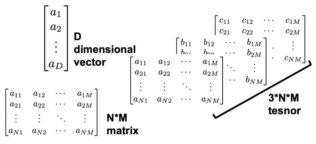
When you study data science or machine learning, usually you should start with understanding the algorithms with 2 or 3 dimensional data, and you can apply those ideas to any D dimensional data. But of course you cannot visualize D dimensional data anymore, and you always have to be careful of what happens if you expand degree of dimension.

Conversely it is also important to reduce dimension to understand abstract high dimensional stuff in 2 or 3 dimensional space, which are close to our everyday sense. That means dimension reduction is one powerful way of data visualization.

In this blog series I am going to explain meanings of dimension itself in machine learning context and algorithms for dimension reductions, such as PCA, LDA, and t-SNE, with 2 or 3 dimensional visible data. Along with that, I am going to delve into the meaning of calculations so that you can understand them in more like everyday-life sense.

This article series is going to be roughly divided into the contents below.

Curse of Dimensionality
Rethinking linear algebra: visualizing linear transformations and eigen vector
The algorithm known as PCA and my taxonomy of linear dimension reductions
Rethinking linear algebra part two: ellipsoids in data science
Autoencoder as dimension reduction (to be published soon)
t-SNE (to be published soon)

I hope you could see that reducing dimension is one of the fundamental approaches in data science or machine learning.

Simple RNN: the first foothold for understanding LSTM

June 17, 2020/in Artificial Intelligence, Data Science, Deep Learning, Machine Learning, Main Category, Mathematics/by Yasuto Tamura

*In this article “Densely Connected Layers” is written as “DCL,” and “Convolutional Neural Network” as “CNN.”

In the last article, I mentioned “When it comes to the structure of RNN, many study materials try to avoid showing that RNNs are also connections of neurons, as well as DCL or CNN.” Even if you manage to understand DCL and CNN, you can be suddenly left behind once you try to understand RNN because it looks like a different field. In the second section of this article, I am going to provide a some helps for more abstract understandings of DCL/CNN , which you need when you read most other study materials.

My explanation on this simple RNN is based on a chapter in a textbook published by Massachusetts Institute of Technology, which is also recommended in some deep learning courses of Stanford University.

First of all, you should keep it in mind that simple RNN are not useful in many cases, mainly because of vanishing/exploding gradient problem, which I am going to explain in the next article. LSTM is one major type of RNN used for tackling those problems. But without clear understanding forward/back propagation of RNN, I think many people would get stuck when they try to understand how LSTM works, especially during its back propagation stage. If you have tried climbing the mountain of understanding LSTM, but found yourself having to retreat back to the foot, I suggest that you read through this article on simple RNNs. It should help you to gain a solid foothold, and you would be ready for trying to climb the mountain again.

*This article is the second article of “A gentle introduction to the tiresome part of understanding RNN.”

1, A brief review on back propagation of DCL.

Simple RNNs are straightforward applications of DCL, but if you do not even have any ideas on DCL forward/back propagation, you will not be able to understand this article. If you more or less understand how back propagation of DCL works, you can skip this first section.

Deep learning is a part of machine learning. And most importantly, whether it is classical machine learning or deep learning, adjusting parameters is what machine learning is all about. Parameters mean elements of functions except for variants. For example when you get a very simple function $f(x)=a + bx + cx^2 + dx^3$ , then $x$ is a variant, and $a, b, c, d$ are parameters. In case of classical machine learning algorithms, the number of those parameters are very limited because they were originally designed manually. Such functions for classical machine learning is useful for features found by humans, after trial and errors(feature engineering is a field of finding such effective features, manually). You adjust those parameters based on how different the outputs(estimated outcome of classification/regression) are from supervising vectors(the data prepared to show ideal answers).

In the last article I said neural networks are just mappings, whose inputs are vectors, matrices, or sequence data. In case of DCLs, inputs are vectors. Then what’s the number of parameters ? The answer depends on the the number of neurons and layers. In the example of DCL at the right side, the number of the connections of the neurons is the number of parameters(Would you like to try to count them? At least I would say “No.”). Unlike classical machine learning you no longer need to do feature engineering, but instead you need to design networks effective for each task and adjust a lot of parameters.

*I think the hype of AI comes from the fact that neural networks find features automatically. But the reality is difficulty of feature engineering was just replaced by difficulty of designing proper neural networks.

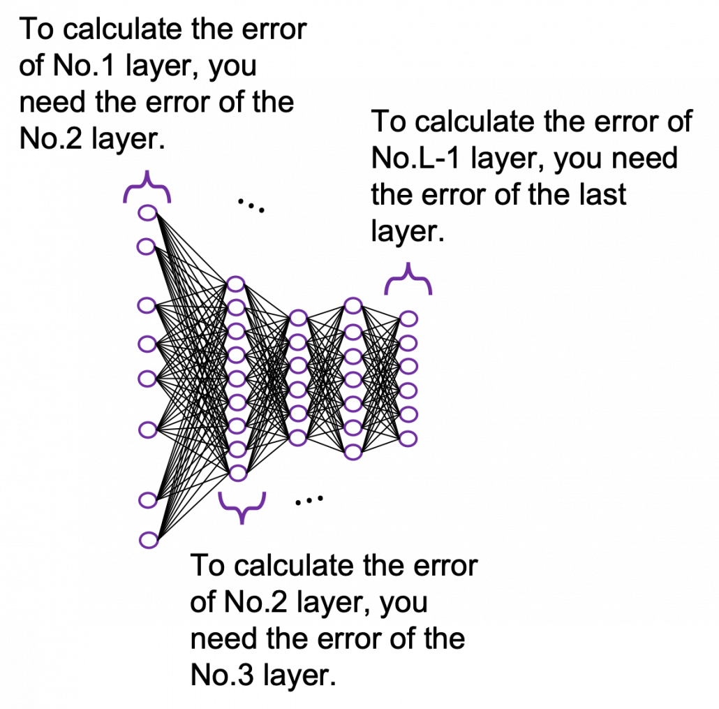
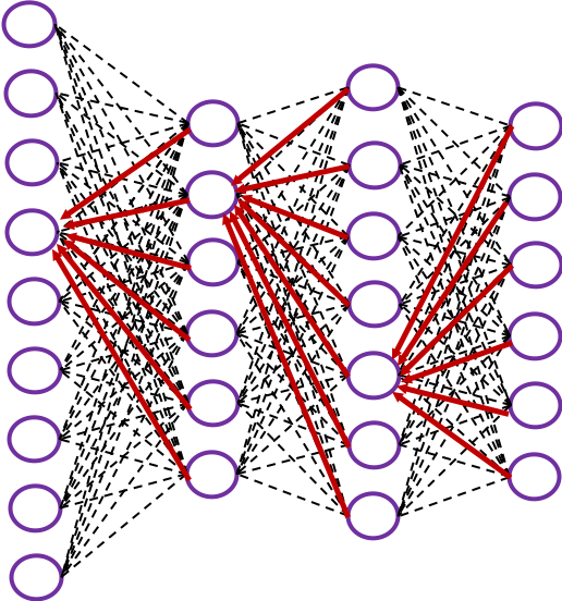
It is easy to imagine that you need an efficient way to adjust those parameters, and the method is called back propagation (or just backprop). As long as it is about DCL backprop, you can find a lot of well-made study materials on that, so I am not going to cover that topic precisely in this article series. Simply putting, during back propagation, in order to adjust parameters of a layer you need errors in the next layer. And in order calculate the errors of the next layer, you need errors in the next next layer.

*You should not think too much about what the “errors” exactly mean. Such “errors” are defined in this context, and you will see why you need them if you actually write down all the mathematical equations behind backprops of DCL.

The red arrows in the figure shows how errors of all the neurons in a layer propagate backward to a neuron in last layer. The figure shows only some sets of such errors propagating backward, but in practice you have to think about all the combinations of such red arrows in the whole back propagation(this link would give you some ideas on how DCLs work).

These points are minimum prerequisites for continuing reading this RNN this article. But if you are planning to understand RNN forward/back propagation at an abstract/mathematical level that you can read academic papers, I highly recommend you to actually write down all the equations of DCL backprop. And if possible you should try to implement backprop of three-layer DCL.

2, Forward propagation of simple RNN

*For better understandings of the second and third section, I recommend you to download an animated PowerPoint slide which I prepared. It should help you understand simple RNNs.

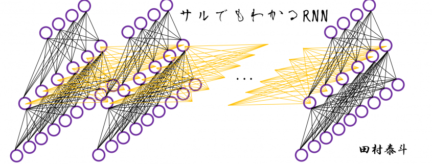
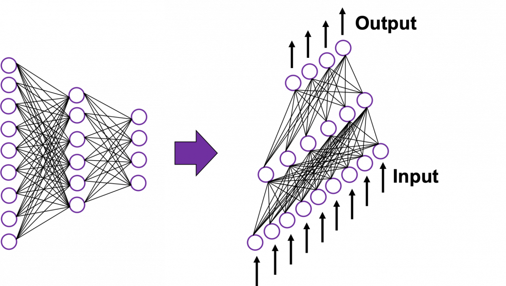
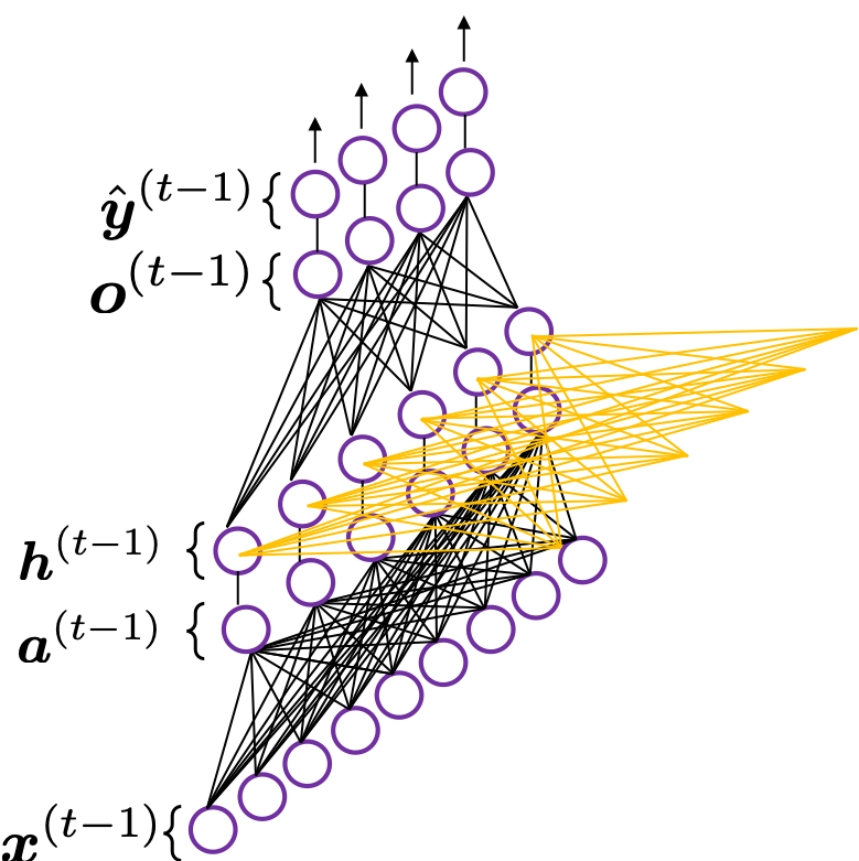
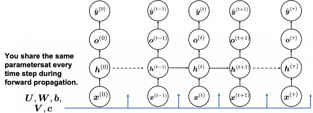
In fact the simple RNN which we are going to look at in this article has only three layers. From now on imagine that inputs of RNN come from the bottom and outputs go up. But RNNs have to keep information of earlier times steps during upcoming several time steps because as I mentioned in the last article RNNs are used for sequence data, the order of whose elements is important. In order to do that, information of the neurons in the middle layer of RNN propagate forward to the middle layer itself. Therefore in one time step of forward propagation of RNN, the input at the time step propagates forward as normal DCL, and the RNN gives out an output at the time step. And information of one neuron in the middle layer propagate forward to the other neurons like yellow arrows in the figure. And the information in the next neuron propagate forward to the other neurons, and this process is repeated. This is called recurrent connections of RNN.

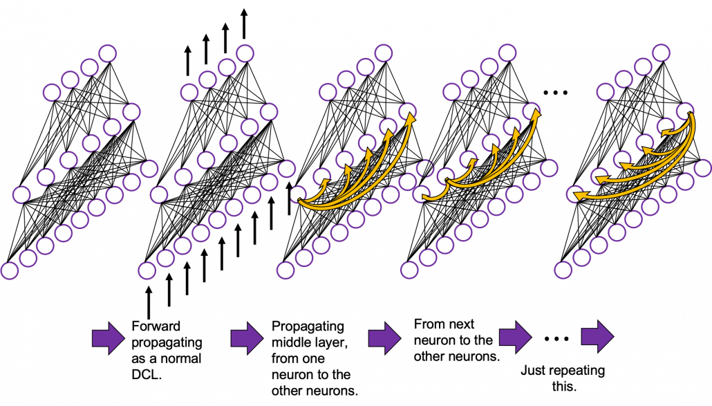
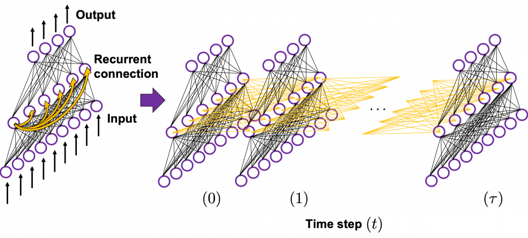
*To be exact we are just looking at a type of recurrent connections. For example Elman RNNs have simpler recurrent connections. And recurrent connections of LSTM are more complicated.

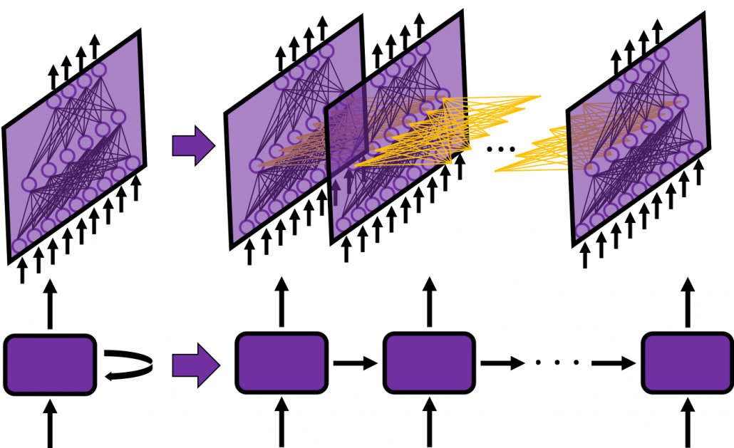
Whether it is a simple one or not, basically RNN repeats this process of getting an input at every time step, giving out an output, and making recurrent connections to the RNN itself. But you need to keep the values of activated neurons at every time step, so virtually you need to consider the same RNNs duplicated for several time steps like the figure below. This is the idea of unfolding RNN. Depending on contexts, the whole unfolded DCLs with recurrent connections is also called an RNN.

In many situations, RNNs are simplified as below. If you have read through this article until this point, I bet you gained some better understanding of RNNs, so you should little by little get used to this more abstract, blackboxed way of showing RNN.

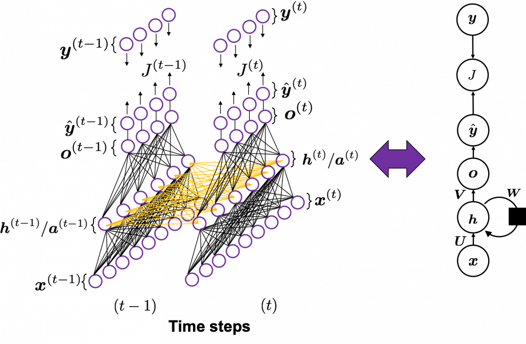
You have seen that you can unfold an RNN, per time step. From now on I am going to show the simple RNN in a simpler way, based on the MIT textbook which I recomment. The figure below shows how RNN propagate forward during two time steps $(t-1), (t)$ .

The input $\boldsymbol{x}^{(t-1)}$ at time step $(t-1)$ propagate forward as a normal DCL, and gives out the output $\hat{\boldsymbol{y}} ^{(t)}$ (The notation on the $\boldsymbol{y} ^{(t)}$ is called “hat,” and it means that the value is an estimated value. Whatever machine learning tasks you work on, the outputs of the functions are just estimations of ideal outcomes. You need to adjust parameters for better estimations. You should always be careful whether it is an actual value or an estimated value in the context of machine learning or statistics). But the most important parts are the middle layers.

*To be exact I should have drawn the middle layers as connections of two layers of neurons like the figure at the right side. But I made my figure closer to the chart in the MIT textbook, and also most other study materials show the combinations of the two neurons before/after activation as one neuron.

$\boldsymbol{a}^{(t)}$ is just linear summations of $\boldsymbol{x}^{(t)}$ (If you do not know what “linear summations” mean, please scroll this page a bit), and $\boldsymbol{h}^{(t)}$ is a combination of activated values of $\boldsymbol{a}^{(t)}$ and linear summations of $\boldsymbol{h}^{(t-1)}$ from the last time step, with recurrent connections. The values of $\boldsymbol{h}^{(t)}$ propagate forward in two ways. One is normal DCL forward propagation to $\hat{\boldsymbol{y}} ^{(t)}$ and $\boldsymbol{o}^{(t)}$ , and the other is recurrent connections to $\boldsymbol{h}^{(t+1)}$ .

These are equations for each step of forward propagation.

$\boldsymbol{a}^{(t)} = \boldsymbol{b} + \boldsymbol{W} \cdot \boldsymbol{h}^{(t-1)} + \boldsymbol{U} \cdot \boldsymbol{x}^{(t)}$
$\boldsymbol{h}^{(t)}= g(\boldsymbol{a}^{(t)})$
$\boldsymbol{o}^{(t)} = \boldsymbol{c} + \boldsymbol{V} \cdot \boldsymbol{h}^{(t)}$
$\hat{\boldsymbol{y}} ^{(t)} = f(\boldsymbol{o}^{(t)})$

*Please forgive me for adding some mathematical equations on this article even though I pledged not to in the first article. You can skip the them, but for some people it is on the contrary more confusing if there are no equations. In case you are allergic to mathematics, I prescribed some treatments below.

*Linear summation is a type of weighted summation of some elements. Concretely, when you have a vector $\boldsymbol{x}=(x_0, x_1, x_2)$ , and weights $\boldsymbol{w}=(w_0,w_1, w_2)$ , then $\boldsymbol{w}^T \cdot \boldsymbol{x} = w_0 \cdot x_0 + w_1 \cdot x_1 +w_2 \cdot x_2$ is a linear summation of $\boldsymbol{x}$ , and its weights are $\boldsymbol{w}$ .

*When you see a product of a matrix and a vector, for example a product of $\boldsymbol{W}$ and $\boldsymbol{v}$ , you should clearly make an image of connections between two layers of a neural network. You can also say each element of $\boldsymbol{u}}$ is a linear summations all the elements of $\boldsymbol{v}}$ , and $\boldsymbol{W}$ gives the weights for the summations.

A very important point is that you share the same parameters, in this case $\boldsymbol{\theta \in \{\boldsymbol{U}, \boldsymbol{W}, \boldsymbol{b}, \boldsymbol{V}, \boldsymbol{c} \}}$ , at every time step.

And you are likely to see this RNN in this blackboxed form.

3, The steps of back propagation of simple RNN

In the last article, I said “I have to say backprop of RNN, especially LSTM (a useful and mainstream type or RNN), is a monster of chain rules.” I did my best to make my PowerPoint on LSTM backprop straightforward. But looking at it again, the LSTM backprop part still looks like an electronic circuit, and it requires some patience from you to understand it. If you want to understand LSTM at a more mathematical level, understanding the flow of simple RNN backprop is indispensable, so I would like you to be patient while understanding this step (and you have to be even more patient while understanding LSTM backprop).

This might be a matter of my literacy, but explanations on RNN backprop are very frustrating for me in the points below.

Most explanations just show how to calculate gradients at each time step.
Most study materials are visually very poor.
Most explanations just emphasize that “errors are back propagating through time,” using tons of arrows, but they lack concrete instructions on how actually you renew parameters with those errors.

If you can relate to the feelings I mentioned above, the instructions from now on could somewhat help you. And with the animated PowerPoint slide I prepared, you would have clear understandings on this topic at a more mathematical level.

Backprop of RNN , as long as you are thinking about simple RNNs, is not so different from that of DCLs. But you have to be careful about the meaning of errors in the context of RNN backprop. Back propagation through time (BPTT) is one of the major methods for RNN backprop, and I am sure most textbooks explain BPTT. But most study materials just emphasize that you need errors from all the time steps, and I think that is very misleading and confusing.

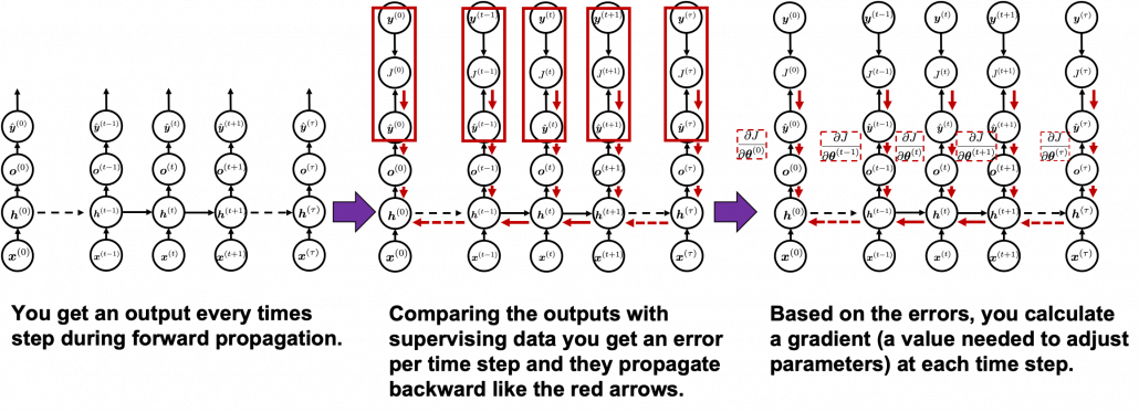
You need all the gradients to adjust parameters, but you do not necessarily need all the errors to calculate those gradients. Gradients in the context of machine learning mean partial derivatives of error functions (in this case $J$ ) with respect to certain parameters, and mathematically a gradient of $J$ with respect to $\boldsymbol{\theta \in \{\boldsymbol{U}, \boldsymbol{W}, \boldsymbol{b}^{(t)}, \boldsymbol{V}, \boldsymbol{c} \}}$ is denoted as $( \frac{\partial J}{\partial \boldsymbol{\theta}} )$ . And another confusing point in many textbooks, including the MIT one, is that they give an impression that parameters depend on time steps. For example some study materials use notations like $\frac{\partial J}{\partial \boldsymbol{\theta}^{(t)}}$ , and I think this gives an impression that this is a gradient with respect to the parameters at time step $(t)$ . In my opinion this gradient rather should be written as $( \frac{\partial J}{\partial \boldsymbol{\theta}} )^{(t)}$ . But many study materials denote gradients of those errors in the former way, so from now on let me use the notations which you can see in the figures in this article.

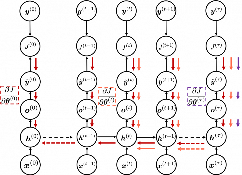
In order to calculate the gradient $\frac{\partial J}{\partial \boldsymbol{x}^{(t)}}$ you need errors from time steps $s (s \geq t) \quad$ (as you can see in the figure, in order to calculate a gradient in a colored frame, you need all the errors in the same color).

*To be exact, in the figure above I am supposed prepare much more arrows in $\tau + 1$ different colors to show the whole process of RNN backprop, but that is not realistic. In the figure I displayed only the flows of errors necessary for calculating each gradient at time step $0, t, \tau$ .

*Another confusing point is that the $\frac{\partial J}{\partial \boldsymbol{\ast ^{(t)}}}, \boldsymbol{\ast} \in \{\boldsymbol{a}^{(t)}, \boldsymbol{h}^{(t)}, \boldsymbol{o}^{(t)}, \dots \}$ are correct notations, because $\boldsymbol{\ast}$ are values of neurons after forward propagation. They depend on time steps, and these are very values which I have been calling “errors.” That is why parameters do not depend on time steps, whereas errors depend on time steps.

As I mentioned before, you share the same parameters at every time step. Again, please do not assume that parameters are different from time step to time step. It is gradients/errors (you need errors to calculate gradients) which depend on time step. And after calculating errors at every time step, you can finally adjust parameters one time, and that’s why this is called “back propagation through time.” (It is easy to imagine that this method can be very inefficient. If the input is the whole text on a Wikipedia link, you need to input all the sentences in the Wikipedia text to renew parameters one time. To solve this problem there is a backprop method named “truncated BPTT,” with which you renew parameters based on a part of a text. )

And after calculating those gradients $\frac{\partial J}{\partial \boldsymbol{\theta}^{(t)}}$ you can take a summation of them: $\frac{\partial J}{\partial \boldsymbol{\theta}}=\sum_{t=0}^{t=\tau}{\frac{\partial J}{\partial \boldsymbol{\theta}^{(t)}}}$ . With this gradient $\frac{\partial J}{\partial \boldsymbol{\theta}}$ , you can finally renew the value of $\boldsymbol{\theta}$ one time.

At the beginning of this article I mentioned that simple RNNs are no longer for practical uses, and that comes from exploding/vanishing problem of RNN. This problem was one of the reasons for the AI winter which lasted for some 20 years. In the next article I am going to write about LSTM, a fancier type of RNN, in the context of a history of neural network history.

A gentle introduction to the tiresome part of understanding RNN

May 1, 2020/in Artificial Intelligence, Data Science, Deep Learning, Machine Learning, Mathematics, Uncategorized/by Yasuto Tamura

Just as a normal conversation in a random pub or bar in Berlin, people often ask me “Which language do you use?” I always answer “LaTeX and PowerPoint.”

I have been doing an internship at DATANOMIQ and trying to make straightforward but precise study materials on deep learning. I myself started learning machine learning in April of 2019, and I have been self-studying during this one-year-vacation of mine in Berlin.

Many study materials give good explanations on densely connected layers or convolutional neural networks (CNNs). But when it comes to back propagation of CNN and recurrent neural networks (RNNs), I think there’s much room for improvement to make the topic understandable to learners.

Many study materials avoid the points I want to understand, and that was as frustrating to me as listening to answers to questions in the Japanese Diet, or listening to speeches from the current Japanese minister of the environment. With the slightest common sense, you would always get the feeling “How?” after reading an RNN chapter in any book.

This blog series focuses on the introductory level of recurrent neural networks. By “introductory”, I mean prerequisites for a better and more mathematical understanding of RNN algorithms.

I am going to keep these posts as visual as possible, avoiding equations, but I am also going to attach some links to check more precise mathematical explanations.

This blog series is composed of five contents.:

Matrix search: Finding the blocks of neighboring fields in a matrix with Python

March 17, 2020/in Mathematics, Python, Tutorial/by Emilia Cheladze

Task

In this article we will look at a solution in python to the following grid search task:

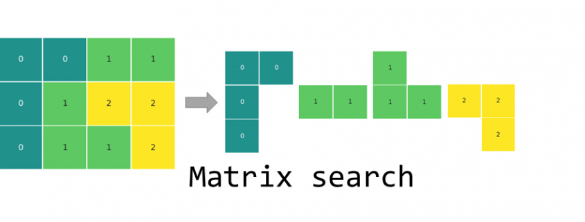
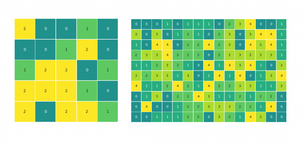
Find the biggest block of adjoining elements of the same kind and into how many blocks the matrix is divided. As adjoining blocks, we will consider field touching by the sides and not the corners.

Input data

For the ease of the explanation, we will be looking at a simple 3×4 matrix with elements of three different kinds, 0, 1 and 2 (see above). To test the code, we will simulate data to achieve different matrix sizes and a varied number of element types. It will also allow testing edge cases like, where all elements are the same or all elements are different.

To simulate some test data for later, we can use the numpy randint() method:

import numpy as np

matrix = [[0,0,1,1], [0,1,2,2], [0,1,1,2]]

matrix_test1 = np.random.randint(3, size = (5,5))

matrix_test2 = np.random.randint(5, size = (10,15))

The code

def find_blocks(matrix):

visited = []

block_list = []

for x in range(len(matrix)):

for y in range(len(matrix[0])):

if (x, y) not in visited:

field_count, visited = explore_block(x, y, visited)

block_list.append(field_count)

return print('biggest block: {0}, number of blocks: {1}'

.format(max(block_list), len(block_list)))

def explore_block(x, y, visited):

queue = {(x,y)}

field_count = 1

while queue:

x,y = queue.pop()

visited.append((x,y))

if x+1<len(matrix) and (x+1,y) not in visited and (x+1,y) not in queue:

if matrix[x+1][y] == matrix[x][y]:

field_count += 1

queue.add((x+1,y))

if x-1>=0 and (x-1,y) not in visited and (x-1,y) not in queue:

if matrix[x-1][y] == matrix[x][y]:

field_count += 1

queue.add((x-1,y))

if y-1>=0 and (x,y-1) not in visited and (x,y-1) not in queue:

if matrix[x][y-1] == matrix[x][y]:

field_count += 1

queue.add((x,y-1))

if y+1<len(matrix[0]) and (x,y+1) not in visited and (x,y+1) not in queue:

if matrix[x][y+1] == matrix[x][y]:

field_count += 1

queue.add((x,y+1))

return field_count, visited

How the code works

In summary, the algorithm loops through all fields of the matrix looking for unseen fields that will serve as a starting point for a local exploration of each block of color – the find_blocks() function. The local exploration is done by looking at the neighboring fields and if they are within the same kind, moving to them to explore further fields – the explore_block() function. The fields that have already been seen and counted are stored in the visited list.

find_blocks() function:

Finds a starting point of a new block
Runs a the explore_block() function for local exploration of the block
Appends the size of the explored block
Updates the list of visited points
Returns the result, once all fields of the matrix have been visited.

explore_block() function:

Takes the coordinates of the starting field for a new block and the list of visited points
Creates the queue set with the starting point
Sets the size of the current block (field_count) to 1
Starts a while loop that is executed for as long as the queue is not empty
1. Takes an element of the queue and uses its coordinates as the current location for further exploration
2. Adds the current field to the visited list
3. Explores the neighboring fields and if they belong to the same block, they are added to the queue
4. The fields are taken off the queue for further exploration one by one until the queue is empty
Returns the field_count of the explored block and the updated list of visited fields

Execute the function

1 2	find_blocks(matrix)

The returned result is biggest block: 4, number of blocks: 4.

Run the test matrices:

find_blocks(matrix_test1)

find_blocks(matrix_test2)

Visualization

The matrices for the article were visualized with the seaborn heatmap() method.

import seaborn as sns

import matplotlib.pyplot as plt

# use annot=False for a matrix without the number labels

sns.heatmap(matrix, annot=True, center = 0, linewidths=.5, cmap = "viridis",

xticklabels=False, yticklabels=False, cbar=False, square=True)

plt.show()

Programmierung für OttoNormalVerbraucher

October 15, 2019/in Business Analytics, Mathematics/by klausbenecke

Facebook und Co. arbeiten daran Nachrichten so aufzubereiten, dass sie emotional noch mehr ansprechen, als ob die gesellschaftliche Situation nicht schon aufgeheizt genug ist. Wir arbeiten daran dem Endnutzer Werkzeuge bereitzustellen um seine rationale Urteilskraft mit Hilfe des Computers zu stärken. Dafür benötigt man möglichst einfache aber dennoch leistungsstarke Programmiersprachen und umfangreiche, vertrauenswürdige, öffentlich zugängliche Informationen in Form von vielgestaltigen großen Tabellen und Dokumenten ähnlich der Wikipedia.

Auch wenn die entwickelte Sprache so einfach wie möglich ist, wird sie im Gegensatz zum Facebookansatz einen gewissen Lernaufwand erfordern.

Eine solche Programmiersprache in Kombination mit vertrauensvollen Daten könnte ein großer Schritt in Richtung einer weiteren Demokratisierung der Gesellschaft werden. Viele Falschnachrichten könnten leicht von jedermann durch entsprechende Fakten oder statistischen Auswertungen paralysiert werden.

Vielleicht kann man die Schaffung einer solchen Programmiersprache mit der Schaffung des ersten Alphabets durch die Phönizier oder der Schaffung des ersten Alphabets mit Vokalen durch die Griechen vergleichen. Hätten diese Völker solche Leistungen vollbringen können ohne diese Voraussetzungen. Ich vermute ohne dieses Alphabet hätte es keine griechische Wissenschaft und Kultur gegeben; vielleicht auch keine griechische Demokratie.

Entwurfskriterien für eine solche Sprache:

Eine mathematische Fundierung ist erforderlich.
Methodisch-didaktische und pragmatische Fragen stehen zunächst vor Effizienzproblemen.
Kurze, lesbare Programme; die wichtigsten Schlüsselworte sollten kurz sein
Einfache, unstrukturierte Programme; Schleifen und allgemeine Rekursionen führen häufig zu schwer lesbaren und schwer änderbaren Programmen;
Universelle Anwendbarkeit; sie muss nicht nur für Relationen (flache einfache Tabellen) sondern auch für strukturierte Tabellen und Dokumente nutzbar sein; sie muss nicht nur für Anfragen an die wichtigsten Systeme sondern auch für vielfältige Berechnungen geeignet sein
Um im Schulunterricht einsetzbar zu sein, muss sie die verschiedenen mathematische Teilgebiete unterstützen, sowie Nutzen für die anderen Fächer bieten
Sie sollte so mächtig sein, dass sie andere Systeme und Sprachen wie Tabellenkalkulation und SQL ersetzen kann.
Aus Endnutzersicht darf es nur ein einheitliches System mit einheitlicher Syntax (Schreibweise) für die Verarbeitung von Massendaten geben, genau wie die Operationen der Einzeldatenverarbeitung (+ – * : sin) standardisiert sind.

Einführung in o++o:

A. Merkel „Jeder Schüler soll neben lesen, rechnen und schreiben auch programmieren können.“

o++o (ausführlich ottoPS) ist eine tabellenorientierte Programmiersprache mit funktionalen Möglichkeiten, die auf Schleifen verzichtet. Dennoch ist o++o sehr ausdrucksstark und man kann mit ihr nicht nur kompakte Anfragen sondern auch vielfältige Berechnungen für strukturierte Tabellen und strukturierte Dokumente bewerkstelligen.

o++o benutzt viele mathematische Konzepte, daher sehen wir die Hauptvorteile der Vermittlung im Mathematikunterricht, genau wie die wesentlichen Fähigkeiten für die Nutzung des Taschenrechners in Mathematik vermittelt werden. o++o verwendet insbesondere folgende Konzepte: Kollektion (Menge, Multimenge, Liste); Gleichheit und Inklusionsbeziehungen dieser; Tupel; leistungsfähige Operationen zum Selektieren; Berechnen; Restrukturieren; Sortieren und Aggregieren (Summe; Durchschnitt; …),… .

Tabellenkalkulationsprogramme wie EXCEL und die Datenbankstandardabfragesprache SQL kennen keine strukturierten Schemen und Tabellen. Erste Tests mit Vorschulkindern lassen vermuten, dass man mit strukturierten Tabellen leichter rechnen kann als mit Dezimalzahlen. Wir wollen einige o++o-Beispielprogramme anfügen:

1. Berechne den Wert eines einfachen Terms.

2*3+4

* und + haben jeweils 2 Inputwerte. Zunächst wird 2*3 (6) berechnet. Die 6 ist erster Inputwert von +, so dass sich insgesamt 24 ergibt. Hier wird also einfach von links nach rechts gerechnet.

2. Schreibe den Term cos³(sin²(3.14159)) in o++o.

pi sin hoch 2 cos hoch 3

Unserer Meinung nach ist der Ausgangsterm für Otto Normalverbraucher schwer zu lesen. Man beginnt mit pi geht nach links bis zum sin dann nach rechts zum hoch 2 jetzt bewegt man sich wieder nach links zum cos und abschließend nach rechts zum hoch 3. Diese Schreibweise wurde sicher eingeführt um Klammern zu sparen. Eigentlich müsste der Ausgangsterm um unmissverständlich zu sein, folgendes Aussehen haben:

(cos((sin(3.14159))²))³

Das ist sicher noch schwerer zu lesen und man bewegt sich noch mehr von links nach rechts und umgekehrt.

3. Schreibe den Term sin²(x)+cos³(y) in o++o.

X sin hoch 2 + (Y cos hoch 3)

oder

X sin hoch 2

+ Y cos hoch 3

Man könnte alle Terme in o++o ohne Klammern schreiben, allerdings müssten dann bestimmte Terme mehrzeilig geschrieben werden.

4. Wie berechnet man den Term 2+3:4*5 ?

2+(3:(4*5))=2 3/20

2+((3:4)*5)=5 ¾

o++o: ((2+3):4)*5=6 1/4

Man erkennt, dass man mit der Schulweisheit Punktrechnung geht vor Strichrechnung noch nicht auskommt. Man benötigt die Regel „von links nach rechts“ zusätzlich.

5. Berechne den Durchschnitt mehrerer Noten.

1 2 3 1 2 ++:

Vom methodischen Standpunkt kann man dieses Programm noch verbessern, indem man die Klammern für Listen hinzufügt: [1 2 3 1 2] ++:

Man erkennt jetzt, dass die Durchschnittsoperation ++: einen Inputwert, nämlich eine Liste besitzt und dass ++: diesem einen Inputwert nachgestellt wird. Da die Nutzer in der Regel nicht viel tippen wollen, gehen wir davon aus, dass die erste Notation in Praxis häufiger benutzt werden wird.

6. Berechne die Durchschnitte einer strukturierten Tabelle noten.tab für jedes Fach.

noten.tab

DUR:=NOTEl ++:

noten.tab könnte so aussehen:

FACH,NOTEl l
Ma 1 2 1 3 1 2
Phy 4 3 2 2 1

…

Hierbei kürzt l Liste ab. D.h., noten.tab ist eine einfache strukturierte Tabelle (Liste), die zu jedem Fach eine Liste von Noten enthält. Um Platz zu sparen, wählen wir auch hier die methodisch nicht optimale Darstellung. Wie FACH ist auch NOTE ein Spaltenname, so dass noten.tab eigentlich so dargestellt werden müsste:

FACH,NOTEl l

Ma 1 2 1 3 1 2
Phy 4 3 2 2 1

Das Ergebnis der Anfrage wieder im „tab-Format“:

FACH, DUR, NOTEl l
Ma 1.66666666667 1 2 1 3 1 2
Phy 2.4 4 3 2 2 1

7. Bilde die Summe der Zahlen von 1 bis 100 (Aufgabe von Gauß Klasse 5).

1 .. 100 ++

Wie die Addition und die Multiplikation besitzt .. zwei Inputwerte (1 und 100). Als Zwischenergebnis entsteht die Liste

ZAHLl
1 2 3 4 5 6 7 8 9 10 11 12 13 14 15 16 17 18 19 20 21 22 23
24 25 26 27 28 29 30 31 32 33 34 35 36 37 38 39 40 41 42 43
44 45 46 47 48 49 50 51 52 53 54 55 56 57 58 59 60 61 62 63
64 65 66 67 68 69 70 71 72 73 74 75 76 77 78 79 80 81 82 83
84 85 86 87 88 89 90 91 92 93 94 95 96 97 98 99 100

,deren Zahlen dann aufsummiert werden, so dass sich 5050 ergibt.

8. Berechne näherungsweise das Maximum der Sinus-Funktion im Intervall [1 2].

1 … 2!0.001 sin max

… benötigt 3 Inputwerte: 1. den Anfangswert 1, den Endwert 2 und die Schrittweite 0.001. Es entstehen hierbei die Zahlen 1 1.001 1.002 1.003 …1.999 2.

Auf jede der Zahlen wird die Sinusfunktion angewandt, sodass wieder 1001 Zahlen entstehen. Auf diese Liste wird dann die Funktion max (Maximum) angewandt. Obwohl es sich hierbei um ein Näherungsverfahren handelt, kommt der exakte Wert 1 heraus, wenn die Schrittweite weiter verfeinert wird. sin und max haben jeweils einen Inputwert (hier eine Liste) aber der Outputwert von sin ist wieder eine Liste und max erzeugt lediglich eine Zahl, da es sich hier um eine Aggregationsfunktion handelt. Der zweite und der dritte Inputwert einer dreistelligen Operation (oben …) wird jeweils durch ein „!“ getrennt. Das ist in o++o nötig, da das Komma für die Paarbildung bereits vergeben ist und das Leerzeichen bereits Listenelemente trennt.

9. Berechne näherungsweise das Minimum des Polynoms X³ + 4 X² -3 X+2 im Intervall [0 2] mit zugehörigem X-Wert.

[X! 0 … 2!0.001]

Y:= X polynom [1 4 -3 2]

MINI:= Yl min

avec Y = MINI

avec ist französisch und bezeichnet eine Selektion. Ein konkretes Polynom von einer Variablen X hat stets nur einen Inputwert, der für X eingesetzt wird. polynom in Zeile 2 ist dagegen allgemeiner und hat 2 Inputwerte:

Den Inputwert für X, der hier alle Zahlen, die in der ersten Zeile generiert wurden, annimmt.
Eine Liste von Zahlen, die den Koeffizienten des konkreten Polynoms entspricht.

Durch die ersten Zeile entsteht eine Liste von Zahlen, die alle den Namen X bekommen haben. Das erkennt man am besten in der xml bzw. ment-Repräsentation:

Gesamtergebnis:
MINI, (X, Y l)

1.481482037 0.333 1.481482037

10. Berechne eine Nullstelle der Cosinus Funktion im Intervall [1 2] näherungsweise.

[X! 1 … 2!0.0001]

avec X cos < 0

avec X pos = 1

Hier verbleiben nach der ersten Selektion nur die X-Werte mit Funktionswert kleiner 0. Von diesen wird im zweiten Schritt der erste Wert ausgewählt. Da wir wissen, dass cos nur eine Nullstelle im betrachteten Intervall besitzt, wird diese durch das Ergebnis angenähert. pos kürzt Position ab, so dass das erste Paar der verbliebenen Paare selektiert wird.

11. Berechne das Gesamtwachstum, wenn 5 Jahreswachstumszahlen gegeben sind. Runde das Ergebnis auf eine Stelle nach dem Komma.

[W! 0 1.5 2.1 1.3 0.4 1.2]

ACCU:= first 100. next ACCU pred *(W:100+1) at W

rnd 1

Die Ergebnistabelle:

[W! 0 1.5 2.1 1.3 0.4 1.2]
ACCU:= first 100. next ACCU pred *(W:100+1) at W
rnd 1
Die Ergebnistabelle:
W, ACCU l
0. 100.
1.5 101.5
2.1 103.6
1.3 105.
0.4 105.4
1.2 106.7

Der erste ACCU-Wert ergibt sich durch den Ausdruck hinter first (100.). Für den zweiten Wert wird für ACCU pred der Wert 100. eingesetzt und der Term nach next bewertet. Es ergibt sich 101.5. Diese Zahl wird wieder in ACCU pred eingesetzt und der next-Term erneut berechnet (rund 103.6),… bis der letzte W-Wert erreicht ist. pred ist der predecessor (Vorgänger).

12. Berechne die Fläche unter der Sinuskurve im Intervall [0, pi] näherungsweise.

0 … pi!0.0001 sin * 0.0001 ++

Hierbei werden nacheinander alle Zahlen zwischen 0 und pi generiert, dann von jeder Zahl der Sinus berechnet und anschließend jede Zahl mit 0.0001 multipliziert. Es entstehen 31415 Rechteckflächen, die abschließend addiert werden.

13. Berechne den DurchschnittsBMI pro Alter und den BMI pro Person und Alter für alle Personen über 20.

<TAB!
NAME, LAENGE, (ALTER, GEWICHT l) l
Klaus        1.68 18 61 30 65 56 80
Rolf       1.78 40 72
Kathi         1.70 18 55 40 70
Walleri     1.00 3 16
Viktoria   1.61 13 51
Bert          1.72 18 66 30 70
!TAB>

avec NAME! 20<ALTER
BMI:= GEWICHT : LAENGE : LAENGE
gib ALTER,BMIAVG,(NAME,BMI m) m BMIAVG:= BMI ! ++:
rnd 2 #rundet alle Zahlen der Tabelle auf 2 Stellen nach dem Punkt

Die TAB-Klammern deuten an, dass die eingeschlossenen Daten der TAB-Darstellung entsprechen.

Die obige Bedingung selektiert Personen-Sätze, d.h. NAME,LAENGE,(ALTER,GEWICHT l) Tupel (strukturierte Tupel bzw. Strupel). Da eine Personen mehrere ALTER-Angaben besitzt, muss quantifiziert werden. NAME! 20 <ALTER selektiert demnach alle Personen, die einen entsprechenden Alterseintrag besitzen. D.h., der Existenzquantor wird nicht geschrieben, gehört aber zu jeder Bedingung. In diesem kleinen Beispiel könnte man die Selektion natürlich auch per Hand realisieren.

Resultat:

ALTER, BMIAVG, (NAME, BMI m) m

18 20.98 Bert 22.31

Kathi 19.03

Klaus 21.61

30 23.35 Bert 23.66

Klaus 23.03

40 23.47 Kathi 24.22

Rolf 22.72

56 28.34 Klaus 28.34

Das Endergebnis kann beispielsweise durch einfaches Klicken als Säulendiagramm dargestellt werden. Das Beispiel zeigt, dass man eine Hierarchie einfach durch Angabe des gewünschten Schemas umkehren kann. Im Ergebnis ist der Name dem Alter untergeordnet.

Es wird insbesondere deutlich, dass die Aufgaben ohne Kenntnisse der Differential- und Integral-rechnung gelöst werden können. Mit o++o kann der Mathematikunterricht in vielfältiger Weise unterstützt werden. Das reicht von Klasse 7 oder tiefer bis zur Klassenstufe 12. Es betrifft: Rechnen mit natürlichen Zahlen, Dezimalzahlen, näherungsweise Berechnung von Nullstellen beliebiger Funktionen, Ableitung, Flächen unter Kurven, Extremwerte (kann wahrscheinlich bereits in der Sekundarschule gelehrt werden), Wahrscheinlichkeitsrechnung, … . Mit o++o können Dinge in einfacher Weise berechnet werden, die sonst nur theoretisch abgehandelt werden. Dadurch kann das Verständnis der Konzepte wesentlich verbessert, erweitert und vertieft werden. Weitere Informationen zu o++o finden Sie unter ottops.de (Z.B. „o++o auf 8 Seiten“ ist eine kurze Einführung).

Wir glauben, dass o++o besondere Vorteile für den Mathematik- und Informatikunterricht bietet aber auch in den anderen Fächern sinnvoll genutzt werden kann.

Simple Linear Regression: Mathematics explained with implementation in numpy

August 18, 2019/in Data Mining, Data Science, Machine Learning, Mathematics, Python/by Aakash Chugh

Simple Linear Regression

Being in the field of data science, we all are familiar with at least some of the measures shown in figure 1.1 (generated in python using statsmodels). But do we really understand how these measures are being calculated? or what is the math behind these measures? In this article, I hope that I can answer these questions for you. This article will start from the fundamentals of simple linear regression but by the end of this article, you will get an idea of how to program this in numpy (python library).

Fig. 1.1

Simple linear regression is a very simple approach for supervised learning where we are trying to predict a quantitative response Y based on the basis of only one variable x. Here x is an independent variable and Y is our dependent variable. Assuming that there is a linear relationship between our independent and dependent variable we can represent this relationship as:

Y = mx+c

where m and c are two unknown constants that represent the slope and the intercept of our linear model. Together, these constants are also known as parameters or coefficients. If you want to visualize these parameters see figure 1.2.

Fig. 1.2

Please note that we can only calculate the estimates of these parameters thus we have to rewrite our linear equation like:

$\widehat{y} = \widehat{m}x + \widehat{c}$

here y-hat represents a prediction of Y (actual value) based on x. Once we have found the estimates of these parameters, the equation can be used to predict the future value of Y provided a new/test value of x.

How to find the estimate of these parameters?

Let’s assume we have ‘n’ observations and for each independent variable value we have a value for dependent variable like this:

(x1,y1), (x2,y2),……,(xn,yn). Our goal is to find the best values of these parameters so the line in fig 1.1 should be as close as possible to the data points and we will be using the most common approach of Ordinary least squares to do that. This best fit is found by minimizing the residual sum of squared errors which can be calculated as below:

$RSS = {(y_1-\widehat{y1}})^2+{(y_2-\widehat{y2}})^2 +…..+{(y_n-\widehat{yn}})^2$

$RSS = {(y_1-\widehat{c}-{\widehat m_1x_1})}^2+ {(y_2-\widehat{c}-{\widehat m_1x_2})}^2 +…..+{(y_n-\widehat{c}-{\widehat m_1x_n})}^2$

where

$m_1 = \frac{\sum_i^n (x_i-\bar x)(y_i-\bar y)}{\sum_i^n (x_i-\bar x)^{2}}$

and

$\widehat{c} = \bar y - \widehat{m_1} \bar x$

Measures to evaluate our regression model

We can use two measures to evaluate our simple linear regression model:

Residual Standard Error (RSE)

According to the book An Introduction to Statistical Learning with Applications in R (James, et al., 2013, pp. 68-71) explains RSE as an estimate of the standard deviation of the error ϵ and can be calculated as:

$RSE = \sqrt{\frac{1}{n-2}\sum_i^n(y_i-\widehat y_i)^2}$

R square

It is not always clear what is a good score for RSE so we use R square as an alternative to measuring the performance of our model. Please note that there are other measures also which we will discuss in my next article about multiple linear regression. We will also cover the difference between the R square and adjusted R square. The formula for R square can be seen below.

$R^2 =1- \frac{\sum_i^n(y_i-\widehat y_i)^2}{(y_i-\bar y)^2}$

Now that we have covered the theoretical part of simple linear regression, let’s write these formulas in python (numpy).

Python implementation

To implement this in python first we need a dataset on which we can work on. The dataset that we are going to use in this article is Advertising data and can be downloaded from here. Before we start the analysis we will use pandas library to load the dataset as a dataframe (see code below).

**Please check your path of the advertising file.

import pandas as pd

import math

import numpy as np

df = pd.read_csv("Advertising.csv")

To show the first five rows of the dataset use df.head() and you will see output like this:

Let me try to explain what are we have to do here, we have the dataset of an ad company which has three different advertising channels TV, radio and newspaper. This company regularly invests in these channels and track their sales over time. However, the time variable is not present in this csv file. Anyway, this company wants to know how much sales will be impacted if they spent a certain amount on any of their advertising channels. As this is the case for simple linear regression we will be using only one predictor TV to fit our model. From here we will go step by step.

Step 1: Define the dependent and independent variable

1 2	x = df.TV # Independent variable y= df.sales # Dependent variable

Step 2: Define a function to find the slope (m)

def slr_slope(x,y):

slope = ((x-x.mean())*(y-y.mean())).sum()/(np.square(x-x.mean())).sum()

return(slope)

m = slr_slope(x,y) # Using the function defined in the above cell

0.047536640433019736

So, when we applied the function in our current dataset we got a slope of 0.0475.

Step 3: Define a function to find the intercept (c)

def slr_intercept(x,y):

c = y.mean()-(m*x.mean())

return(c)

c = slr_intercept(x,y)

7.032593549127698

and an intercept of 7.0325

Once we have the values for slope and intercept, it is now time to define functions to calculate the residual sum of squares (RSS) and the metrics we will use to evaluate our linear model i.e. residual standard error (RSE) and R-square.

Step 4: Define a function to find residual sum of squares (RSS)

def slr_rss(x,y):

rss = (np.square(y-c-(m*x))).sum()

return(rss)

rss = slr_rss(x,y)

rss

2102.5305831313512

As we discussed in the theory section that it is very hard to evaluate a model based on RSS as we can never generalize the thresholds for RSS and hence we need to settle for other measures.

Step 5: Define a function to calculate residual standard error (RSE)

def slr_rse(x,y):

rss = (np.square(y-c-(m*x))).sum()

rse = np.sqrt(rss/(len(x)-2))

return(rse)

rse = slr_rse(x,y)

rse

3.2586563686504624

Step 6: Define a function to find R-square

def slr_r2(x,y):

tss = np.square((y-y.mean())).sum()

rss = (np.square(y-c-(m*x))).sum()

r2 = 1 - (rss/tss)

return(r2)

r2 = slr_r2(x,y)

0.611875050850071

Here, we see that R-square offers an advantage over RSE as it always lies between 0 and 1, which makes it easier to evaluate our linear model. If you want to understand more about what constitutes a good measure of R-square you can read the explanation given in the book An introduction to statistical learning (mentioned this above also).

The final step now would be to define a function which can be used to predict our sales on the amount of budget spend on TV.

def slr_prediction(slope,test_datapoint,intercept):

y = ((slope*test_datapoint)+intercept)

return(y)

Now, let’s say if the advertising budget for TV is 1500 USD, what would be their sales?

slr_prediction(m,1500,intercept=c)

78.3375541986573

Our linear model predicted that if the ad company would spend 1500 USD they will see an increase of 78 units. If you want to go through the whole code you can find the jupyter notebook here. In this notebook, I have also made a class wrapper at the end of this linear model. It will be really hard to explain the whole logic why I did it here, so I will keep that for another post.In the next article, I will explain the mathematics behind Multiple Linear Regression and how we can implement that in python. Please let me know if you have any question in the comments section. Thank you for reading !!

1. My taxonomy on linear dimension reduction

2. PCA

3. Fitting orthogonal axes on data

4. Practical three dimensional example of PCA

Appendix: Playing with my toy PCA on MNIST dataset

1, The mainstream ways of explaining diagonalization.

2, Linear transformations

3, Eigen vectors as coordinate system

4, Eigen vectors of positive semidefinite matrices

5, Orthonormal matrices and rotation of vectors

Advantages Of KNN

Where KNN Are Mostly Used

Choosing The Right Value For K

Your Step-By-Step Guide For Choosing The Value Of K

Conclusion

This article series is going to be roughly divided into the contents below.

1, A brief review on back propagation of DCL.

2, Forward propagation of simple RNN

3, The steps of back propagation of simple RNN

This blog series is composed of five contents.:

Task

Find the biggest block of adjoining elements of the same kind and into how many blocks the matrix is divided. As adjoining blocks, we will consider field touching by the sides and not the corners.

Input data

The code

How the code works

Execute the function

Visualization

Simple Linear Regression

How to find the estimate of these parameters?

Measures to evaluate our regression model

Residual Standard Error (RSE)

R square

Python implementation

Step 1: Define the dependent and independent variable

Step 2: Define a function to find the slope (m)

Step 3: Define a function to find the intercept (c)

Step 4: Define a function to find residual sum of squares (RSS)

Step 5: Define a function to calculate residual standard error (RSE)

Step 6: Define a function to find R-square

Interesting links

Pages

Categories

Archive