Positional encoding, residual connections, padding masks: covering the rest of Transformer components

This is the fourth article of my article series named “Instructions on Transformer for people outside NLP field, but with examples of NLP.”

1 Wrapping points up so far

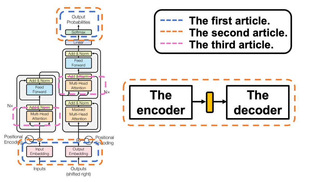
This article series has already covered a great deal of the Transformer mechanism. Whether you have read my former articles or not, I bet you are more or less lost in the course of learning Transformer model. The left side of the figure below is from the original paper on Transformer model, and my previous articles explained the parts in each colored frame. In the first article, I  mainly explained how language is encoded in deep learning task and how that is evaluated.

This is more of a matter of inputs and the outputs of deep learning networks, which are in blue dotted frames in the figure. They are not so dependent on types of deep learning NLP tasks. In the second article, I explained seq2seq models, which are encoder-decoder models used in machine translation. Seq2seq models can can be simplified like the figure in the orange frame. In the article I mainly explained seq2seq models with RNNs, but the purpose of this article series is ultimately replace them with Transformer models. In the last article, I finally wrote about some actual components of Transformer models: multi-head attention mechanism. I think this mechanism is the core of Transformed models, and I did my best to explain it with a whole single article, with a lot of visualizations. However, there are still many elements I have not explained.

First, you need to do positional encoding to the word embedding so that Transformer models can learn the relations of the positions of input tokens. At least I was too stupid to understand what this is only with the original paper on Transformer. I am going to explain this algorithm in illustrative ways, which I needed to self-teach it. The second point is residual connections.

The last article has already explained multi-head attention, as precisely as I could do, but I still have to say I covered only two multi-head attention parts in a layer of Transformer model, which are in pink frames. During training, you have to mask some tokens at the decoder part so that some of tokens are invisible, and masked multi-head attention enables that.

You might be tired of the words “queries,” “keys,” and “values,” if you read the last article. But in fact that was not enough. When you think about applying Transformer in other tasks, such as object detection or image generation, you need to reconsider what the structure of data and how “queries,” “keys,” and “values,” correspond to each elements of the data, and probably one of my upcoming articles would cover this topic.

2 Why Transformer?

One powerful strength of Transformer model is its parallelization. As you saw in the last article, Trasformer models enable calculating relations of tokens to all other tokens, on different standards, independently in each head. And each head requires very simple linear transformations. In case of RNN encoders, if an input has tokens, basically you have to wait for time steps to finish encoding the input sentence. Also, at the time step the RNN cell retains the information at the time step only via recurrent connections. In this way you cannot attend to tokens in the earlier time steps, and this is obviously far from how we compare tokens in a sentence. You can bring information backward by bidirectional connection s in RNN models, but that all the more deteriorate parallelization of the model. And possessing information via recurrent connections, like a telephone game, potentially has risks of vanishing gradient problems. Gated RNN, such as LSTM or GRU mitigate the problems by a lot of nonlinear functions, but that adds to computational costs. If you understand multi-head attention mechanism, I think you can see that Transformer solves those problems.

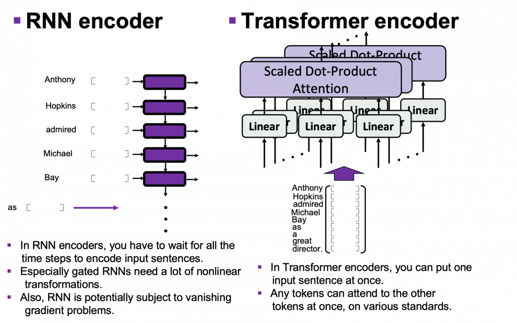
I guess this is closer to when you speak a foreign language which you are fluent in. You wan to say something in a foreign language, and you put the original sentence in your mother tongue in the “encoder” in your brain. And you decode it, word by word, in the foreign language. You do not have to wait for the word at the end in your language, or rather you have to consider the relations of of a chunk of words to another chunk of words, in forward and backward ways. This is crucial especially when Japanese people speak English. You have to make the conclusion clear in English usually with the second word, but the conclusion is usually at the end of the sentence in Japanese.

3 Positional encoding

I explained disadvantages of RNN in the last section, but RNN has been a standard algorithm of neural machine translation. As I mentioned in the fourth section of the first article of my series on RNN, other neural nets like fully connected layers or convolutional neural networks cannot handle sequence data well. I would say RNN could be one of the only algorithms to handle sequence data, including natural language data, in more of classical methods of time series data processing.

*As I explained in this article, the original idea of RNN was first proposed in 1997, and I would say the way it factorizes time series data is very classical, and you would see similar procedures in many other algorithms. I think Transformer is a successful breakthrough which gave up the idea of processing sequence data time step by time step.

You might have noticed that multi-head attention mechanism does not explicitly uses the the information of the orders or position of input data, as it basically calculates only the products of matrices. In the case where the input is “Anthony Hopkins admired Michael Bay as a great director.”, multi head attention mechanism does not uses the information that “Hopkins” is the second token, or the information that the token two time steps later is “Michael.” Transformer tackles this problem with an almost magical algorithm named positional encoding.

In order to learn positional encoding, you should first think about what kind of encoding is ideal. According to this blog post, ideal encoding of positions of tokens have the following features.

• Positional encoding of one token deterministically represents the position of the token.
• The actual values of positional encoding should not be too big compared to the values of elements of embedding vectors.
• Positional encodings of different tokens should successfully express their relative positions.

The most straightforward way to give the information of position is implementing the index of times steps , but if you naively give the term to the data, the term could get too big compared to the values of data ,for example when the sequence data is 100 time steps long. The next straightforward idea is compressing the idea of time steps to for example the range . With this approach, however, the resolution of encodings can vary depending on the length of the input sequence data. Thus these naive approaches do not meet the requirements above, and I guess even conventional RNN-based models were not so successful in these points.

*I guess that is why attention mechanism of RNN seq2seq models, which I explained in the second article, was successful. You can constantly calculate the relative positions of decoder tokens compared to the encoder tokens.

Positional encoding, to me almost magically, meets the points I have mentioned. However the explanation of positional encoding in the original paper of Transformer is unkindly brief. It says you can encode positions of tokens with the following vector , , where . is the dimension of word embedding. The heat map below is the most typical type of visualization of positional encoding you would see everywhere, and in this case , and is discrete number which varies from to , thus the heat map blow is equal to a matrix, whose elements are from to . Each row of the graph corresponds to one token, and you can see that lower dimensional part is constantly changing like waves. Also it is quite easy to encode an input with this positional encoding: assume that you have a matrix of an input sentence composed of 50 tokens, each of which is a 256 dimensional vector, then all you have to do is just adding the heat map below to the matrix.

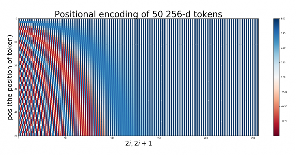
Concretely writing down, the encoding of the 256-dim token at   is .

You should see this encoding more as pairs of circles rather than dimensional vectors. When you fix the , the index of the depth of each encoding, you can extract a 2 dimensional vector . If you constantly change the value , the vector rotates clockwise on the unit circle in the figure below.

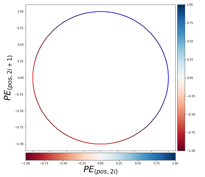
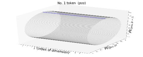
Also, the deeper the dimension of the embedding is, I mean the bigger the index is, the smaller the frequency of rotation is. I think the video below is a more intuitive way to see how each token is encoded with positional encoding. You can see that the bigger is, that is the more tokens an input has, the deeper part positional encoding starts to rotate on the circles.

Very importantly, the original paper of Transformer says, “We chose this function because we hypothesized it would allow the model to easily learn to attend by relative positions, since for any fixed offset , can be represented as a linear function of .” For each circle at any depth, I mean for any , the following simple equation holds:

The matrix is a simple rotation matrix, so if is fixed the rotation only depends on , how many positions to move forward or backward. Then we get a very important fact: as the changes ( is a discrete number), each point rotates in proportion to the offset of “pos,” with different frequencies depending on the depth of the circles. The deeper the circle is, the smaller the frequency is. That means, this type of positional encoding encourages Transformer models to learn definite and relative positions of tokens with rotations of those circles, and the values of each element of the rotation matrices are from to , so they do not get bigger no matter how many tokens inputs have.

For example when an input is “Anthony Hopkins admired Michael Bay as a great director.”, a shift from the token “Hopkins” to “Bay” is a rotation matrix  , where . Also the shift from “Bay” to “great” has the same rotation.

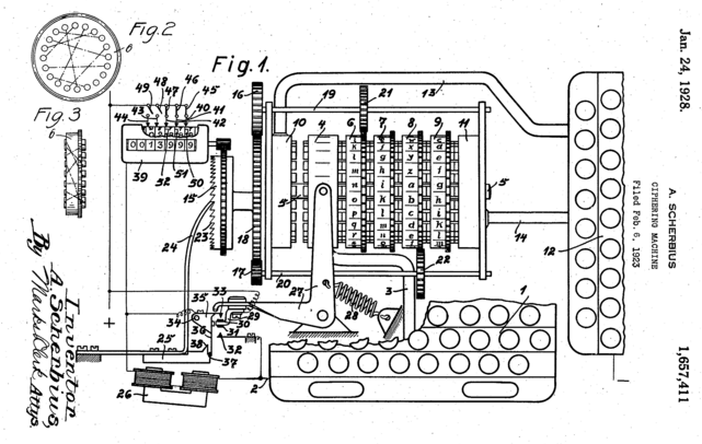
*Positional encoding reminded me of Enigma, a notorious cipher machine used by Nazi Germany. It maps alphabets to different alphabets with different rotating gear connected by cables. With constantly changing gears and keys, it changed countless patterns of alphabetical mappings, every day, which is impossible for humans to solve. One of the first form of computers was invented to break Enigma.

*As far as I could understand from “Imitation Game (2014).”

*But I would say Enigma only relied on discrete deterministic algebraic mapping of alphabets. The rotations of positional encoding is not that tricky as Enigma, but it can encode both definite and deterministic positions of much more variety of tokens. Or rather I would say AI algorithms developed enough to learn such encodings with subtle numerical changes, and I am sure development of NLP increased the possibility of breaking the Turing test in the future.

5 Residual connections

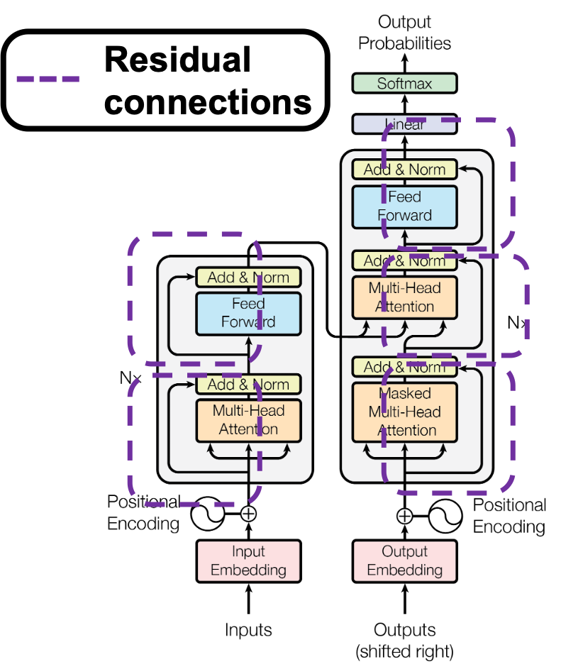
If you naively stack neural networks with simple implementation, that would suffer from vanishing gradient problems during training. Back propagation is basically multiplying many gradients, so

One way to mitigate vanishing gradient problems is quite easy: you have only to make a bypass of propagation. You would find a lot of good explanations on residual connections, so I am not going to explain how this is effective for vanishing gradient problems in this article.

In Transformer models you add positional encodings to the input only in the first layer, but I assume that the encodings remain through the layers by these bypass routes, and that might be one of reasons why Transformer models can retain information of positions of tokens.

6 Masked multi-head attention

Even though Transformer, unlike RNN, can attend to the whole input sentence at once, the decoding process of Transformer-based translator is close to RNN-based one, and you are going to see that more clearly in the codes in the next article. As I explained in the second article, RNN decoders decode each token only based on the tokens the have generated so far. Transformer decoder also predicts the output sequences autoregressively one token at a time step, just as RNN decoders. I think it easy to understand this process because RNN decoder generates tokens just as you connect RNN cells one after another, like connecting rings to a chain. In this way it is easy to make sure that generating of one token in only affected by the former tokens. On the other hand, during training Transformer decoders, you input the whole sentence at once. That means Transformer decoders can see the whole sentence during training. That is as if a student preparing for a French translation test could look at the whole answer French sentences. It is easy to imagine that you cannot prepare for the French test effectively if you study this way. Transformer decoders also have to learn to decode only based on the tokens they have generated so far.

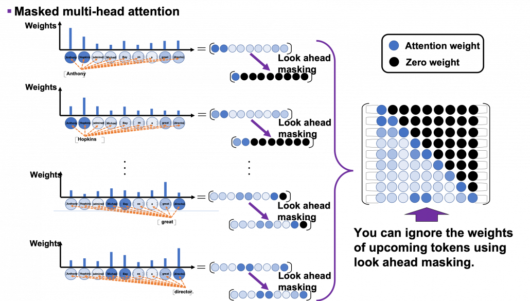
In order to properly train a Transformer-based translator to learn such decoding, you have to hide the upcoming tokens in target sentences during training. During calculating multi-head attentions in each Transformer layer, if you keep ignoring the weights from up coming tokens like in the figure below, it is likely that Transformer models learn to decode only based on the tokens generated so far. This is called masked multi-head attention.

*I am going to take an input “Anthonly Hopkins admire Michael Bay as a great director.” as an example of calculating masked multi-head attention mechanism, but this is supposed to be in the target laguage. So when you train an translator from English to German, in practice you have to calculate masked multi-head atetntion of “Anthony Hopkins hat Michael Bay als einen großartigen Regisseur bewundert.”

As you can see from the whole architecture of Transformer, you only need to consider masked multi-head attentions of of self-attentions of the input sentences at the decoder side. In order to concretely calculate masked multi-head attentions, you need a technique named look ahead masking. This is also quite simple. Just as well as the last article, let’s take an example of calculating self attentions of an input “Anthony Hopkins admired Michael Bay as a great director.” Also in this case you just calculate multi-head attention as usual, but when you get the histograms below, you apply look ahead masking to each histogram and delete the weights from the future tokens. In the figure below the black dots denote zero, and the sum of each row of the resulting attention map is also one. In other words, you get a lower triangular matrix, the sum of whose each row is 1.

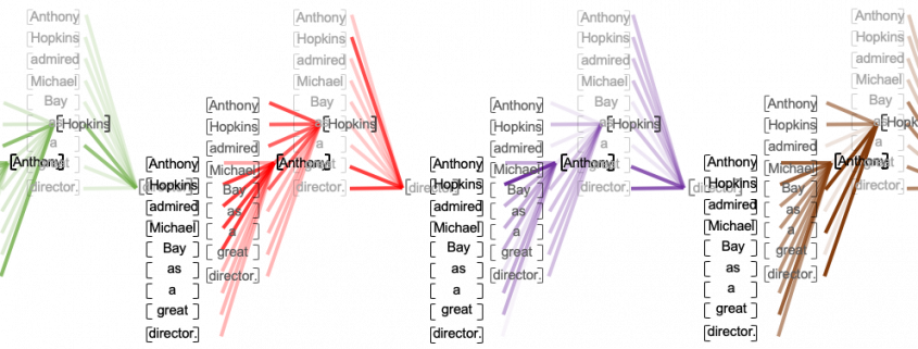
Also just as I explained in the last article, you reweight vlaues with the triangular attention map. The figure below is calculating a transposed masked multi-head attention because I think it is a more straightforward way to see how vectors are reweighted in multi-head attention mechanism.

When you closely look at how each column of the transposed multi-head attention is reweighted, you can clearly see that the token is reweighted only based on the tokens generated so far.

*If you are still not sure why you need such masking in multi-head attention of target sentences, you should proceed to the next article for now. Once you check the decoding processes of Transformer-based translators, you would see why you need masked multi-head attention mechanism on the target sentence during training.

If you have read my articles, at least this one and the last one, I think you have gained more or less clear insights into how each component of Transfomer model works. You might have realized that each components require simple calculations. Combined with the fact that multi-head attention mechanism is highly parallelizable, Transformer is easier to train, compared to RNN.

In this article, we are going to see how masking of multi-head attention is implemented and how the whole Transformer structure is constructed. By the end of the next article, you would be able to create a toy English-German translator with more or less clear understanding on its architecture.

About Author

Yasuto Tamura

Data Science Intern at DATANOMIQ.
Majoring in computer science. Currently studying mathematical sides of deep learning, such as densely connected layers, CNN, RNN, autoencoders, and making study materials on them. Also started aiming at Bayesian deep learning algorithms.

See author's posts