Wie Maschinen uns verstehen: Natural Language Understanding
Foto von Sebastian Bill auf Unsplash.
Natural Language Understanding (NLU) ist ein Teilbereich von Computer Science, der sich damit beschäftigt natürliche Sprache, also beispielsweise Texte oder Sprachaufnahmen, verstehen und verarbeiten zu können. Das Ziel ist es, dass eine Maschine in der gleichen Weise mit Menschen kommunizieren kann, wie es Menschen untereinander bereits seit Jahrhunderten tun.
Was sind die Bereiche von NLU?
Eine neue Sprache zu erlernen ist auch für uns Menschen nicht einfach und erfordert viel Zeit und Durchhaltevermögen. Wenn eine Maschine natürliche Sprache erlernen will, ist es nicht anders. Deshalb haben sich einige Teilbereiche innerhalb des Natural Language Understandings herausgebildet, die notwendig sind, damit Sprache komplett verstanden werden kann.
Diese Unterteilungen können auch unabhängig voneinander genutzt werden, um einzelne Aufgaben zu lösen:
- Speech Recognition versucht aufgezeichnete Sprache zu verstehen und in textuelle Informationen umzuwandeln. Das macht es für nachgeschaltete Algorithmen einfacher die Sprache zu verarbeiten. Speech Recognition kann jedoch auch alleinstehend genutzt werden, beispielsweise um Diktate oder Vorlesungen in Text zu verwandeln.
- Part of Speech Tagging wird genutzt, um die grammatikalische Zusammensetzung eines Satzes zu erkennen und die einzelnen Satzbestandteile zu markieren.
- Named Entity Recognition versucht innerhalb eines Textes Wörter und Satzbausteine zu finden, die einer vordefinierten Klasse zugeordnet werden können. So können dann zum Beispiel alle Phrasen in einem Textabschnitt markiert werden, die einen Personennamen enthalten oder eine Zeit ausdrücken.
- Sentiment Analysis klassifiziert das Sentiment, also die Gefühlslage, eines Textes in verschiedene Stufen. Dadurch kann beispielsweise automatisiert erkannt werden, ob eine Produktbewertung eher positiv oder eher negativ ist.
- Natural Language Generation ist eine allgemeine Gruppe von Anwendungen mithilfe derer automatisiert neue Texte generiert werden sollen, die möglichst natürlich klingen. Zum Beispiel können mithilfe von kurzen Produkttexten ganze Marketingbeschreibungen dieses Produkts erstellt werden.
Welche Algorithmen nutzt man für NLP?
Die meisten, grundlegenden Anwendungen von NLP können mit den Python Modulen spaCy und NLTK umgesetzt werden. Diese Bibliotheken bieten weitreichende Modelle zur direkten Anwendung auf einen Text, ohne vorheriges Trainieren eines eigenen Algorithmus. Mit diesen Modulen ist ohne weiteres ein Part of Speech Tagging oder Named Entity Recognition in verschiedenen Sprachen möglich.
Der Hauptunterschied zwischen diesen beiden Bibliotheken ist die Ausrichtung. NLTK ist vor allem für Entwickler gedacht, die eine funktionierende Applikation mit Natural Language Processing Modulen erstellen wollen und dabei auf Performance und Interkompatibilität angewiesen sind. SpaCy hingegen versucht immer Funktionen bereitzustellen, die auf dem neuesten Stand der Literatur sind und macht dabei möglicherweise Einbußen bei der Performance.
Für umfangreichere und komplexere Anwendungen reichen jedoch diese Optionen nicht mehr aus, beispielsweise wenn man eine eigene Sentiment Analyse erstellen will. Je nach Anwendungsfall sind dafür noch allgemeine Machine Learning Modelle ausreichend, wie beispielsweise ein Convolutional Neural Network (CNN). Mithilfe von Tokenizern von spaCy oder NLTK können die einzelnen in Wörter in Zahlen umgewandelt werden, mit denen wiederum das CNN als Input arbeiten kann. Auf heutigen Computern sind solche Modelle mit kleinen Neuronalen Netzwerken noch schnell trainierbar und deren Einsatz sollte deshalb immer erst geprüft und möglicherweise auch getestet werden.
Jedoch gibt es auch Fälle in denen sogenannte Transformer Modelle benötigt werden, die im Bereich des Natural Language Processing aktuell state-of-the-art sind. Sie können inhaltliche Zusammenhänge in Texten besonders gut mit in die Aufgabe einbeziehen und liefern daher bessere Ergebnisse beispielsweise bei der Machine Translation oder bei Natural Language Generation. Jedoch sind diese Modelle sehr rechenintensiv und führen zu einer sehr langen Rechenzeit auf normalen Computern.
Was sind Transformer Modelle?
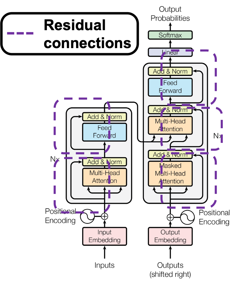
In der heutigen Machine Learning Literatur führt kein Weg mehr an Transformer Modellen aus dem Paper „Attention is all you need“ (Vaswani et al. (2017)) vorbei. Speziell im Bereich des Natural Language Processing sind die darin erstmals beschriebenen Transformer Modelle nicht mehr wegzudenken.
Transformer werden aktuell vor allem für Übersetzungsaufgaben genutzt, wie beispielsweise auch bei www.deepl.com. Darüber hinaus sind diese Modelle auch für weitere Anwendungsfälle innerhalb des Natural Language Understandings geeignet, wie bspw. das Beantworten von Fragen, Textzusammenfassung oder das Klassifizieren von Texten. Das GPT-2 Modell ist eine Implementierung von Transformern, dessen Anwendungen und die Ergebnisse man hier ausprobieren kann.
Was macht den Transformer so viel besser?
Soweit wir wissen, ist der Transformer jedoch das erste Transduktionsmodell, das sich ausschließlich auf die Selbstaufmerksamkeit (im Englischen: Self-Attention) stützt, um Repräsentationen seiner Eingabe und Ausgabe zu berechnen, ohne sequenzorientierte RNNs oder Faltung (im Englischen Convolution) zu verwenden.
Übersetzt aus dem englischen Originaltext: Attention is all you need (Vaswani et al. (2017)).
In verständlichem Deutsch bedeutet dies, dass das Transformer Modell die sogenannte Self-Attention nutzt, um für jedes Wort innerhalb eines Satzes die Beziehung zu den anderen Wörtern im gleichen Satz herauszufinden. Dafür müssen nicht, wie bisher, Recurrent Neural Networks oder Convolutional Neural Networks zum Einsatz kommen.
Was dieser Mechanismus konkret bewirkt und warum er so viel besser ist, als die vorherigen Ansätze wird im folgenden Beispiel deutlich. Dazu soll der folgende deutsche Satz mithilfe von Machine Learning ins Englische übersetzt werden:
„Das Mädchen hat das Auto nicht gesehen, weil es zu müde war.“
Für einen Computer ist diese Aufgabe leider nicht so einfach, wie für uns Menschen. Die Schwierigkeit an diesem Satz ist das kleine Wort „es“, dass theoretisch für das Mädchen oder das Auto stehen könnte. Aus dem Kontext wird jedoch deutlich, dass das Mädchen gemeint ist. Und hier ist der Knackpunkt: der Kontext. Wie programmieren wir einen Algorithmus, der den Kontext einer Sequenz versteht?
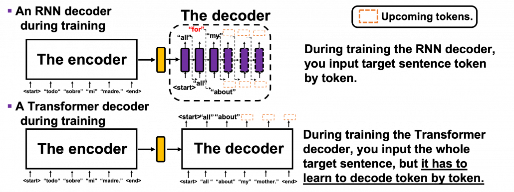
Vor Veröffentlichung des Papers „Attention is all you need“ waren sogenannte Recurrent Neural Networks die state-of-the-art Technologie für solche Fragestellungen. Diese Netzwerke verarbeiten Wort für Wort eines Satzes. Bis man also bei dem Wort „es“ angekommen ist, müssen erst alle vorherigen Wörter verarbeitet worden sein. Dies führt dazu, dass nur noch wenig Information des Wortes „Mädchen“ im Netzwerk vorhanden sind bis den Algorithmus überhaupt bei dem Wort „es“ angekommen ist. Die vorhergegangenen Worte „weil“ und „gesehen“ sind zu diesem Zeitpunkt noch deutlich stärker im Bewusstsein des Algorithmus. Es besteht also das Problem, dass Abhängigkeiten innerhalb eines Satzes verloren gehen, wenn sie sehr weit auseinander liegen.
Was machen Transformer Modelle anders? Diese Algorithmen prozessieren den kompletten Satz gleichzeitig und gehen nicht Wort für Wort vor. Sobald der Algorithmus das Wort „es“ in unserem Beispiel übersetzen will, wird zuerst die sogenannte Self-Attention Layer durchlaufen. Diese hilft dem Programm andere Wörter innerhalb des Satzes zu erkennen, die helfen könnten das Wort „es“ zu übersetzen. In unserem Beispiel werden die meisten Wörter innerhalb des Satzes einen niedrigen Wert für die Attention haben und das Wort Mädchen einen hohen Wert. Dadurch ist der Kontext des Satzes bei der Übersetzung erhalten geblieben.

 and
and 
 , where
  , respectively from English and German corpus, then we learn a mapping
  .
. . Thus
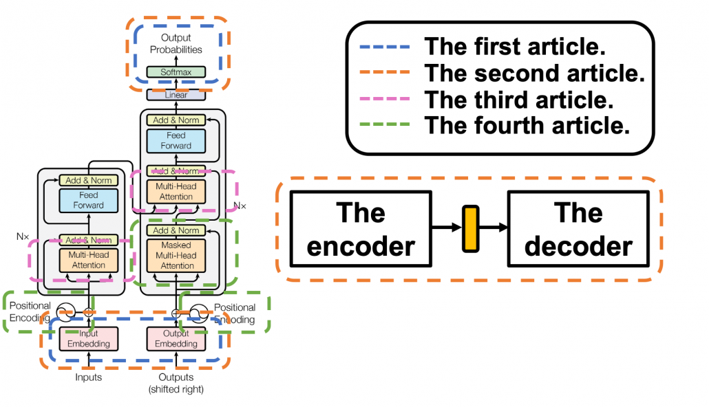
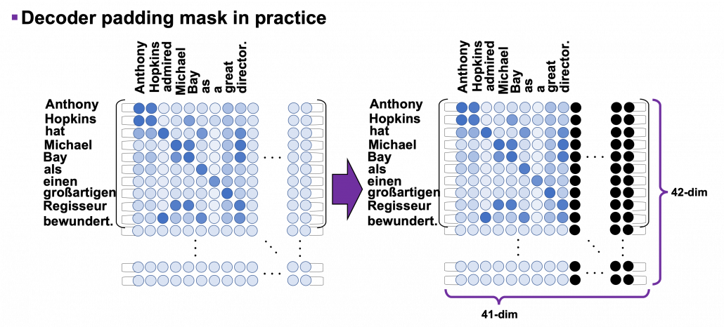
 layers. The decoder part also keeps converting the inputs in the target languages, also through
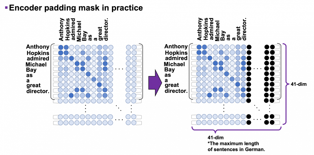
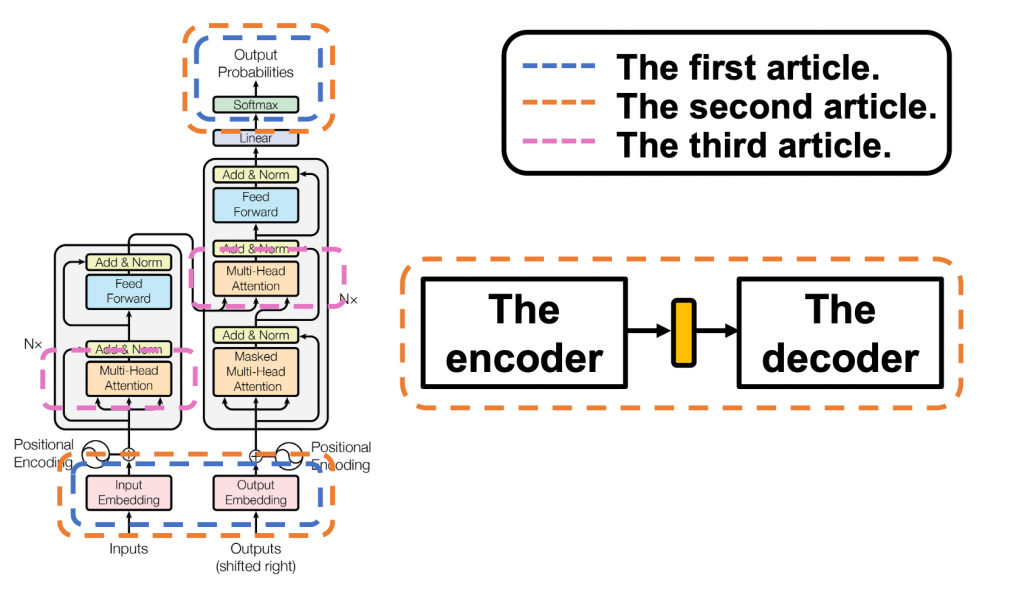
 . In short you stack two fully connected layers and activate it with a ReLU function. Let’s see how point_wise_feed_forward_network() function works in the implementation with some simple codes. As you can see from the number of parameters in each layer of the position wise feed forward neural network, the network does not depend on the length of the sentences.
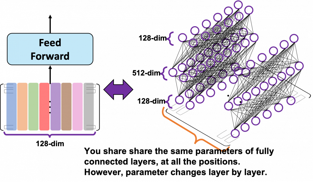
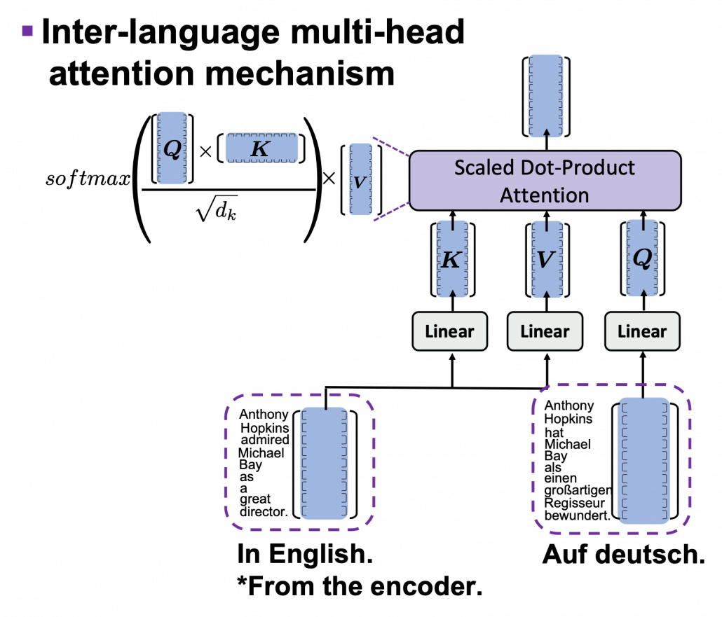
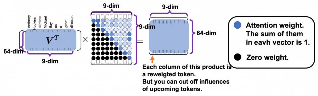
 . In the example above, the resulting multi-head attention map is a
  matrix like in the figure below.
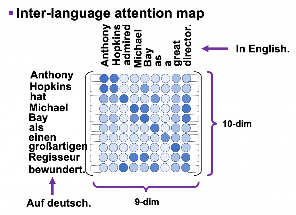
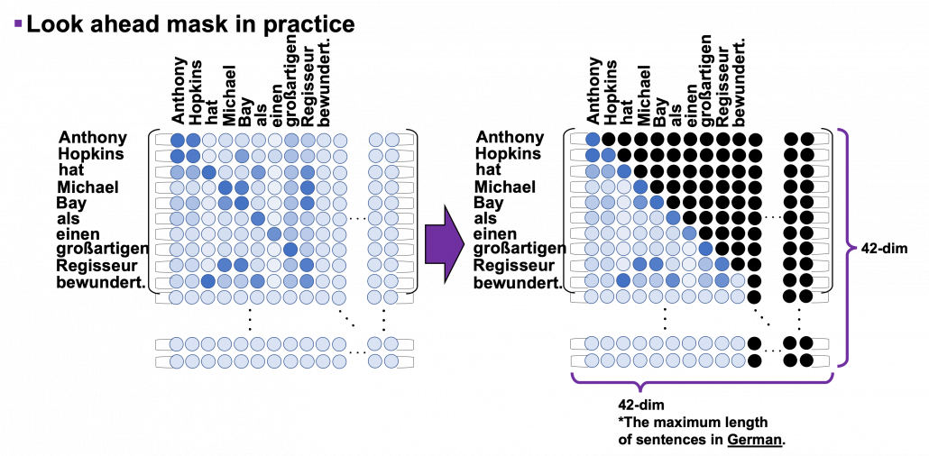
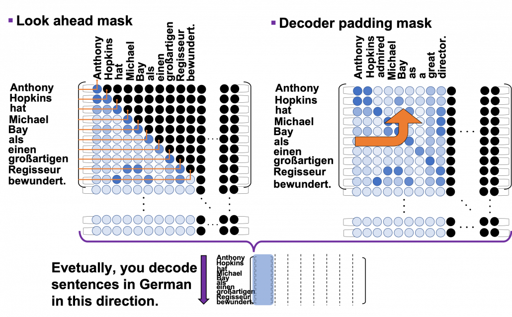
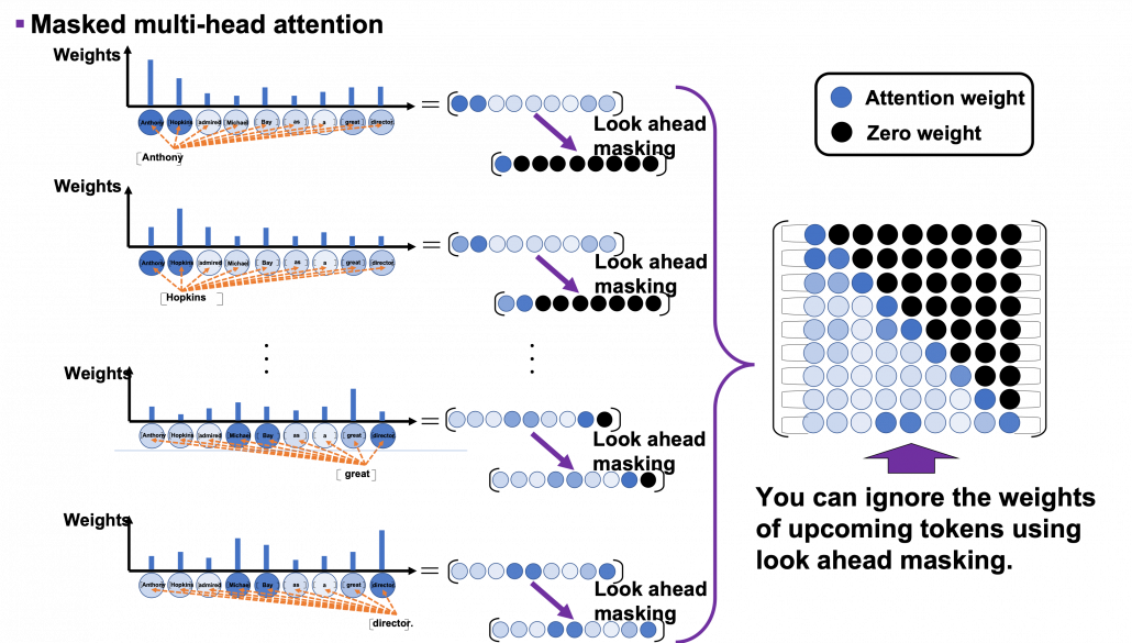
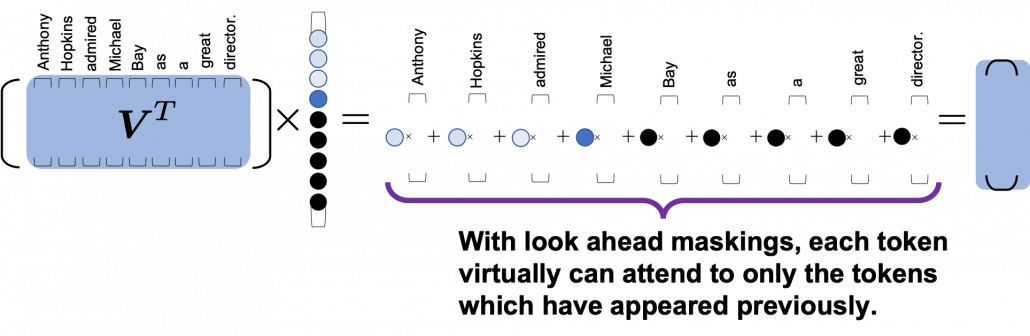
 can depend only on the known outputs at positions less than
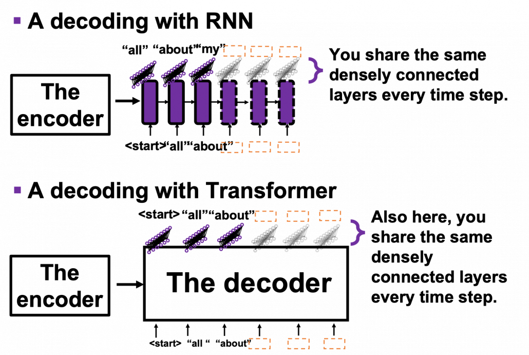
 tokens, basically you have to wait for
  the RNN cell retains the information at the time step
  only via recurrent connections. In this way you cannot attend to tokens in the earlier time steps, and this is obviously far from how we compare tokens in a sentence. You can bring information backward by bidirectional connection s in RNN models, but that all the more deteriorate parallelization of the model. And possessing information via recurrent connections, like a telephone game, potentially has risks of vanishing gradient problems. Gated RNN, such as LSTM or GRU mitigate the problems by a lot of nonlinear functions, but that adds to computational costs. If you understand multi-head attention mechanism, I think you can see that Transformer solves those problems.
 , but if you naively give the term
 ![[0, 1]](https://data-science-blog.com/wp-content/ql-cache/quicklatex.com-caffaae885a1287e3dfc31bfb1cd0694_l3.png "Rendered by QuickLaTeX.com") . With this approach, however, the resolution of encodings can vary depending on the length of the input sequence data. Thus these naive approaches do not meet the requirements above, and I guess even conventional RNN-based models were not so successful in these points.
. With this approach, however, the resolution of encodings can vary depending on the length of the input sequence data. Thus these naive approaches do not meet the requirements above, and I guess even conventional RNN-based models were not so successful in these points. ,
,  , where
  .
.  is the dimension of word embedding. The heat map below is the most typical type of visualization of positional encoding you would see everywhere, and in this case
  , and
, and  is discrete number which varies from
  to
to  , thus the heat map blow is equal to a
  matrix, whose elements are from
  to
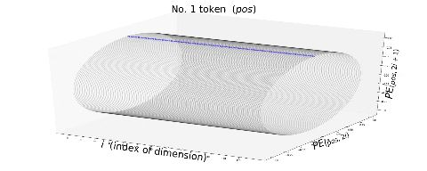
to  . Each row of the graph corresponds to one token, and you can see that lower dimensional part is constantly changing like waves. Also it is quite easy to encode an input with this positional encoding: assume that you have a matrix of an input sentence composed of 50 tokens, each of which is a 256 dimensional vector, then all you have to do is just adding the heat map below to the matrix.
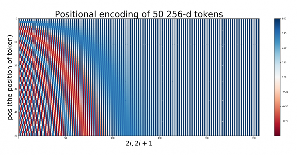

 .
. pairs of circles rather than
 . If you constantly change the value
  rotates clockwise on the unit circle in the figure below.
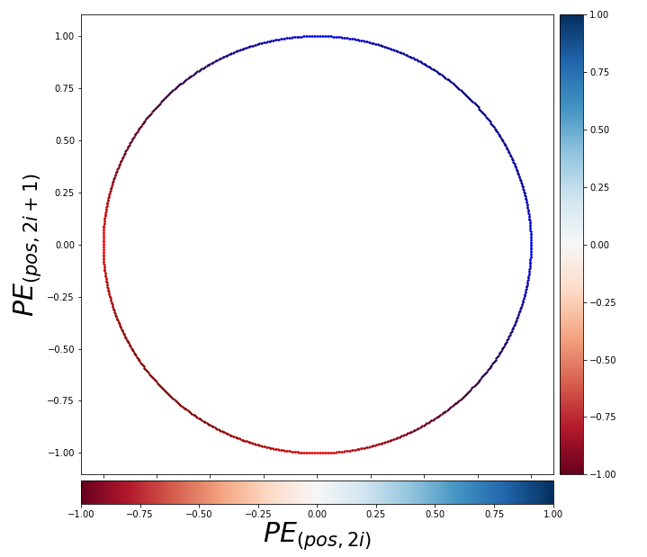
 ,
,  can be represented as a linear function of
  .” For each circle at any depth, I mean for any

 , where
  . Also the shift from “Bay” to “great” has the same rotation.