Simple Linear Regression: Mathematics explained with implementation in numpy
Simple Linear Regression
Being in the field of data science, we all are familiar with at least some of the measures shown in figure 1.1 (generated in python using statsmodels). But do we really understand how these measures are being calculated? or what is the math behind these measures? In this article, I hope that I can answer these questions for you. This article will start from the fundamentals of simple linear regression but by the end of this article, you will get an idea of how to program this in numpy (python library).
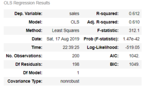
Fig. 1.1
Simple linear regression is a very simple approach for supervised learning where we are trying to predict a quantitative response Y based on the basis of only one variable x. Here x is an independent variable and Y is our dependent variable. Assuming that there is a linear relationship between our independent and dependent variable we can represent this relationship as:
Y = mx+c
where m and c are two unknown constants that represent the slope and the intercept of our linear model. Together, these constants are also known as parameters or coefficients. If you want to visualize these parameters see figure 1.2.
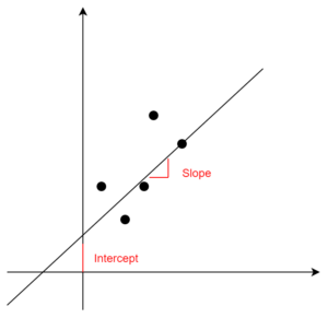
Fig. 1.2
Please note that we can only calculate the estimates of these parameters thus we have to rewrite our linear equation like:

here y-hat represents a prediction of Y (actual value) based on x. Once we have found the estimates of these parameters, the equation can be used to predict the future value of Y provided a new/test value of x.
How to find the estimate of these parameters?
Let’s assume we have ‘n’ observations and for each independent variable value we have a value for dependent variable like this:
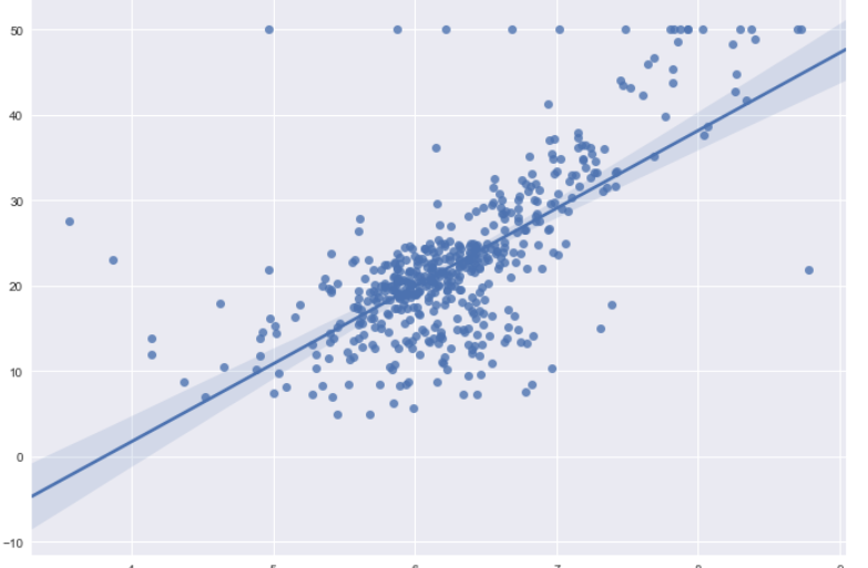
(x1,y1), (x2,y2),……,(xn,yn). Our goal is to find the best values of these parameters so the line in fig 1.1 should be as close as possible to the data points and we will be using the most common approach of Ordinary least squares to do that. This best fit is found by minimizing the residual sum of squared errors which can be calculated as below:

or

where

and

Measures to evaluate our regression model
We can use two measures to evaluate our simple linear regression model:
Residual Standard Error (RSE)
According to the book An Introduction to Statistical Learning with Applications in R (James, et al., 2013, pp. 68-71) explains RSE as an estimate of the standard deviation of the error ϵ and can be calculated as:

R square
It is not always clear what is a good score for RSE so we use R square as an alternative to measuring the performance of our model. Please note that there are other measures also which we will discuss in my next article about multiple linear regression. We will also cover the difference between the R square and adjusted R square. The formula for R square can be seen below.

Now that we have covered the theoretical part of simple linear regression, let’s write these formulas in python (numpy).
Python implementation
To implement this in python first we need a dataset on which we can work on. The dataset that we are going to use in this article is Advertising data and can be downloaded from here. Before we start the analysis we will use pandas library to load the dataset as a dataframe (see code below).
**Please check your path of the advertising file.
|
1 2 3 4 5 6 |
import pandas as pd import math import numpy as np df = pd.read_csv("Advertising.csv") |
To show the first five rows of the dataset use df.head() and you will see output like this:
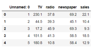
Let me try to explain what are we have to do here, we have the dataset of an ad company which has three different advertising channels TV, radio and newspaper. This company regularly invests in these channels and track their sales over time. However, the time variable is not present in this csv file. Anyway, this company wants to know how much sales will be impacted if they spent a certain amount on any of their advertising channels. As this is the case for simple linear regression we will be using only one predictor TV to fit our model. From here we will go step by step.
Step 1: Define the dependent and independent variable
|
1 2 |
x = df.TV # Independent variable y= df.sales # Dependent variable |
Step 2: Define a function to find the slope (m)
|
1 2 3 |
def slr_slope(x,y): slope = ((x-x.mean())*(y-y.mean())).sum()/(np.square(x-x.mean())).sum() return(slope) |
|
1 2 3 4 5 |
m = slr_slope(x,y) # Using the function defined in the above cell m 0.047536640433019736 |
So, when we applied the function in our current dataset we got a slope of 0.0475.
Step 3: Define a function to find the intercept (c)
|
1 2 3 |
def slr_intercept(x,y): c = y.mean()-(m*x.mean()) return(c) |
|
1 2 3 4 5 |
c = slr_intercept(x,y) c 7.032593549127698 |
and an intercept of 7.0325
Once we have the values for slope and intercept, it is now time to define functions to calculate the residual sum of squares (RSS) and the metrics we will use to evaluate our linear model i.e. residual standard error (RSE) and R-square.
Step 4: Define a function to find residual sum of squares (RSS)
|
1 2 3 |
def slr_rss(x,y): rss = (np.square(y-c-(m*x))).sum() return(rss) |
|
1 2 3 4 5 |
rss = slr_rss(x,y) rss 2102.5305831313512 |
As we discussed in the theory section that it is very hard to evaluate a model based on RSS as we can never generalize the thresholds for RSS and hence we need to settle for other measures.
Step 5: Define a function to calculate residual standard error (RSE)
|
1 2 3 4 |
def slr_rse(x,y): rss = (np.square(y-c-(m*x))).sum() rse = np.sqrt(rss/(len(x)-2)) return(rse) |
|
1 2 3 4 5 |
rse = slr_rse(x,y) rse 3.2586563686504624 |
Step 6: Define a function to find R-square
|
1 2 3 4 5 |
def slr_r2(x,y): tss = np.square((y-y.mean())).sum() rss = (np.square(y-c-(m*x))).sum() r2 = 1 - (rss/tss) return(r2) |
|
1 2 3 4 5 |
r2 = slr_r2(x,y) r2 0.611875050850071 |
Here, we see that R-square offers an advantage over RSE as it always lies between 0 and 1, which makes it easier to evaluate our linear model. If you want to understand more about what constitutes a good measure of R-square you can read the explanation given in the book An introduction to statistical learning (mentioned this above also).
The final step now would be to define a function which can be used to predict our sales on the amount of budget spend on TV.
|
1 2 3 |
def slr_prediction(slope,test_datapoint,intercept): y = ((slope*test_datapoint)+intercept) return(y) |
Now, let’s say if the advertising budget for TV is 1500 USD, what would be their sales?
|
1 2 3 4 |
slr_prediction(m,1500,intercept=c) 78.3375541986573 |
Our linear model predicted that if the ad company would spend 1500 USD they will see an increase of 78 units. If you want to go through the whole code you can find the jupyter notebook here. In this notebook, I have also made a class wrapper at the end of this linear model. It will be really hard to explain the whole logic why I did it here, so I will keep that for another post.In the next article, I will explain the mathematics behind Multiple Linear Regression and how we can implement that in python. Please let me know if you have any question in the comments section. Thank you for reading !!


Leave a Reply
Want to join the discussion?Feel free to contribute!