TensorFlow Archives

How to make a toy English-German translator with multi-head attention heat maps: the overall architecture of Transformer

May 10, 2021/in Artificial Intelligence, Data Mining, Data Science, Data Science Hack, Deep Learning, Insights, Machine Learning, Main Category, Python, Python, TensorFlow, Tools, Tutorial/by Yasuto Tamura

If you have been patient enough to read the former articles of this article series Instructions on Transformer for people outside NLP field, but with examples of NLP, you should have already learned a great deal of Transformer model, and I hope you gained a solid foundation of learning theoretical sides on this algorithm.

This article is going to focus more on practical implementation of a transformer model. We use codes in the Tensorflow official tutorial. They are maintained well by Google, and I think it is the best practice to use widely known codes.

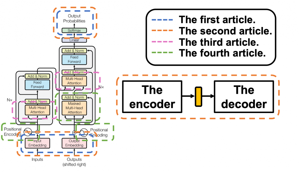
The figure below shows what I have explained in the articles so far. Depending on your level of understanding, you can go back to my former articles. If you are familiar with NLP with deep learning, you can start with the third article.

1 The datasets

I think this article series appears to be on NLP, and I do believe that learning Transformer through NLP examples is very effective. But I cannot delve into effective techniques of processing corpus in each language. Thus we are going to use a library named BPEmb. This library enables you to encode any sentences in various languages into lists of integers. And conversely you can decode lists of integers to the language. Thanks to this library, we do not have to do simplification of alphabets, such as getting rid of Umlaut.

*Actually, I am studying in computer vision field, so my codes would look elementary to those in NLP fields.

The official Tensorflow tutorial makes a Portuguese-English translator, but in article we are going to make an English-German translator. Basically, only the codes below are my original. As I said, this is not an article on NLP, so all you have to know is that at every iteration you get a batch of (64, 41) sized tensor as the source sentences, and a batch of (64, 42) tensor as corresponding target sentences. 41, 42 are respectively the maximum lengths of the input or target sentences, and when input sentences are shorter than them, the rest positions are zero padded, as you can see in the codes below.

*If you just replace datasets and modules for encoding, you can make translators of other pairs of languages.

We are going to train a seq2seq-like Transformer model of converting those list of integers, thus a mapping from a vector to another vector. But each word, or integer is encoded as an embedding vector, so virtually the Transformer model is going to learn a mapping from sequence data to another sequence data. Let’s formulate this into a bit more mathematics-like way: when we get a pair of sequence data $\boldsymbol{X} =$ $(\boldsymbol{x}^{(1)}, \dots, \boldsymbol{x}^{(\tau _x)})$ and $\boldsymbol{Y} =$ $(\boldsymbol{y}^{(1)}, \dots, \boldsymbol{y}^{(\tau _y)})$ , where $\boldsymbol{x}^{(t)} \in \mathbb{R}^{|\mathcal{V}_{\mathcal{X}}|}, \boldsymbol{x}^{(t)} \in \mathbb{R}^{|\mathcal{V}_{\mathcal{Y}}|}$ , respectively from English and German corpus, then we learn a mapping $f: \boldsymbol{X} \to \boldsymbol{Y}$ .

*In this implementation the vocabulary sizes are both $10002$ . Thus $|\mathcal{V}_{\mathcal{X}}|=|\mathcal{V}_{\mathcal{Y}}|=10002$

2 The whole architecture

This article series has covered most of components of Transformer model, but you might not understand how seq2seq-like models can be constructed with them. It is very effective to understand how transformer is constructed by actually reading or writing codes, and in this article we are finally going to construct the whole architecture of a Transforme translator, following the Tensorflow official tutorial. At the end of this article, you would be able to make a toy English-German translator.

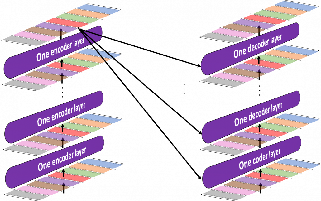
The implementation is mainly composed of 4 classes, EncoderLayer(), Encoder(), DecoderLayer(), and Decoder() class. The inclusion relations of the classes are displayed in the figure below.

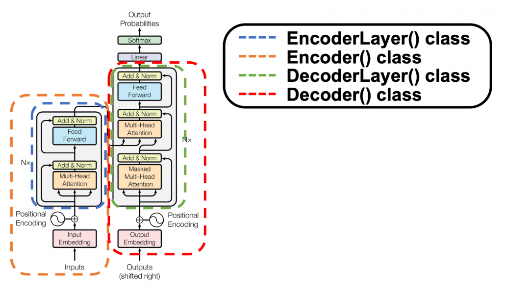
To be more exact in a seq2seq-like model with Transformer, the encoder and the decoder are connected like in the figure below. The encoder part keeps converting input sentences in the original language through $N$ layers. The decoder part also keeps converting the inputs in the target languages, also through $N$ layers, but it receives the output of the final layer of the Encoder at every layer.

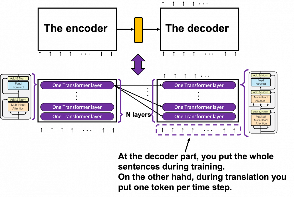
You can see how the Encoder() class and the Decoder() class are combined in Transformer in the codes below. If you have used Tensorflow or Pytorch to some extent, the codes below should not be that hard to read.

3 The encoder

*From now on “sentences” do not mean only the input tokens in natural language, but also the reweighted and concatenated “values,” which I repeatedly explained in explained in the former articles. By the end of this section, you will see that Transformer repeatedly converts sentences layer by layer, remaining the shape of the original sentence.

I have explained multi-head attention mechanism in the third article, precisely, and I explained positional encoding and masked multi-head attention in the last article. Thus if you have read them and have ever written some codes in Tensorflow or Pytorch, I think the codes of Transformer in the official Tensorflow tutorial is not so hard to read. What is more, you do not use CNNs or RNNs in this implementation. Basically all you need is linear transformations. First of all let’s see how the EncoderLayer() and the Encoder() classes are implemented in the codes below.

You might be confused what “Feed Forward” means in this article or the original paper on Transformer. The original paper says this layer is calculated as $FFN(x) =$ $max(0, xW_1 + b_1)W_2 +b_2$ . In short you stack two fully connected layers and activate it with a ReLU function. Let’s see how point_wise_feed_forward_network() function works in the implementation with some simple codes. As you can see from the number of parameters in each layer of the position wise feed forward neural network, the network does not depend on the length of the sentences.

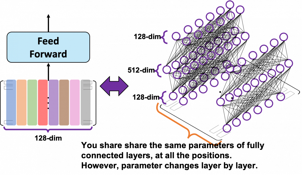
From the number of parameters of the position-wise feed forward neural networks, you can see that you share the same parameters over all the positions of the sentences. That means in the figure above, you use the same densely connected layers at all the positions, in single layer. But you also have to keep it in mind that parameters for position-wise feed-forward networks change from layer to layer. That is also true of “Layer” parts in Transformer model, including the output part of the decoder: there are no learnable parameters which cover over different positions of tokens. These facts lead to one very important feature of Transformer: the number of parameters does not depend on the length of input or target sentences. You can offset the influences of the length of sentences with multi-head attention mechanisms. Also in the decoder part, you can keep the shape of sentences, or reweighted values, layer by layer, which is expected to enhance calculation efficiency of Transformer models.

4, The decoder

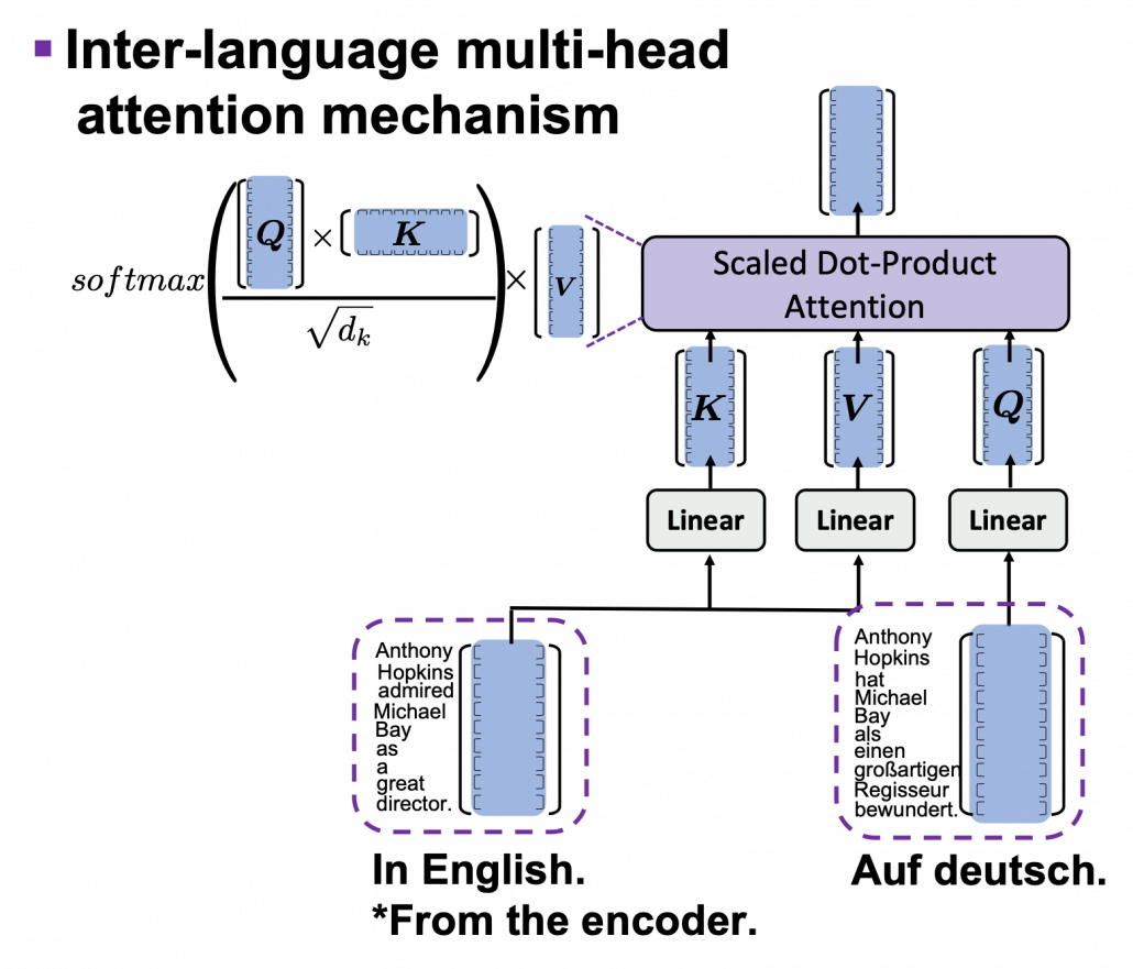
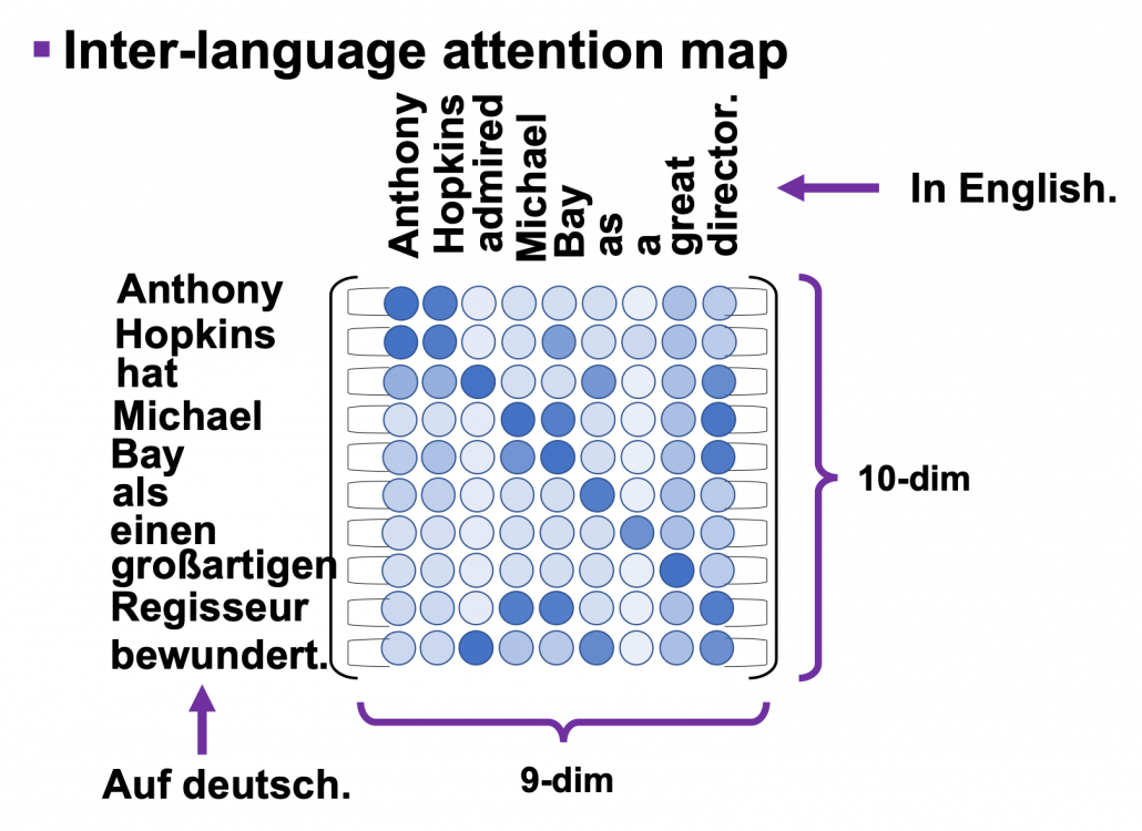
The structures of DecoderLayer() and the Decoder() classes are quite similar to those of EncoderLayer() and the Encoder() classes, so if you understand the last section, you would not find it hard to understand the codes below. What you have to care additionally in this section is inter-language multi-head attention mechanism. In the third article I was repeatedly explaining multi-head self attention mechanism, taking the input sentence “Anthony Hopkins admired Michael Bay as a great director.” as an example. However, as I explained in the second article, usually in attention mechanism, you compare sentences with the same meaning in two languages. Thus the decoder part of Transformer model has not only self-attention multi-head attention mechanism of the target sentence, but also an inter-language multi-head attention mechanism. That means, In case of translating from English to German, you compare the sentence “Anthony Hopkins hat Michael Bay als einen großartigen Regisseur bewundert.” with the sentence itself in masked multi-head attention mechanism (, just as I repeatedly explained in the third article). On the other hand, you compare “Anthony Hopkins hat Michael Bay als einen großartigen Regisseur bewundert.” with “Anthony Hopkins admired Michael Bay as a great director.” in the inter-language multi-head attention mechanism (, just as you can see in the figure above).

*The “inter-language multi-head attention mechanism” is my original way to call it.

I briefly mentioned how you calculate the inter-language multi-head attention mechanism in the end of the third article, with some simple codes, but let’s see that again, with more straightforward figures. If you understand my explanation on multi-head attention mechanism in the third article, the inter-language multi-head attention mechanism is nothing difficult to understand. In the multi-head attention mechanism in encoder layers, “queries”, “keys”, and “values” come from the same sentence in English, but in case of inter-language one, only “keys” and “values” come from the original sentence, and “queries” come from the target sentence. You compare “queries” in German with the “keys” in the original sentence in English, and you re-weight the sentence in English. You use the re-weighted English sentence in the decoder part, and you do not need look-ahead mask in this inter-language multi-head attention mechanism.

Just as well as multi-head self-attention, you can calculate inter-language multi-head attention mechanism as follows: $softmax(\frac{\boldsymbol{Q} \boldsymbol{K} ^T}{\sqrt{d}_k})$ . In the example above, the resulting multi-head attention map is a $10 \times 9$ matrix like in the figure below.

Once you keep the points above in you mind, the implementation of the decoder part should not be that hard.

5 Masking tokens in practice

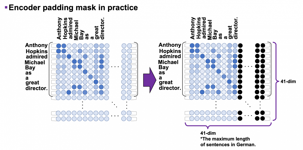
I explained masked-multi-head attention mechanism in the last article, and the ideas itself is not so difficult. However in practice this is implemented in a little tricky way. You might have realized that the size of input matrices is fixed so that it fits the longest sentence. That means, when the maximum length of the input sentences is 41, even if the sentences in a batch have less than 41 tokens, you sample (64, 41) sized tensor as a batch every time (The 64 is a batch size). Let “Anthony Hopkins admired Michael Bay as a great director.”, which has 9 tokens in total, be an input. We have been considering calculating (9, 9) sized attention maps or (10, 9) sized attention maps, but in practice you use (41, 41) or (42, 41) sized ones. When it comes to calculating self attentions in the encoder part, you zero pad self attention maps with encoder padding masks, like in the figure below. The black dots denote the zero valued elements.

As you can see in the codes below, encode padding masks are quite simple. You just multiply the padding masks with -1e9 and add them to attention maps and apply a softmax function. Thereby you can zero-pad the columns in the positions/columns where you added -1e9 to.

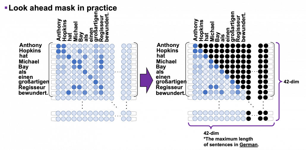
I explained look ahead mask in the last article, and in practice you combine normal padding masks and look ahead masks like in the figure below. You can see that you can compare each token with only its previous tokens. For example you can compare “als” only with “Anthony”, “Hopkins”, “hat”, “Michael”, “Bay”, “als”, not with “einen”, “großartigen”, “Regisseur” or “bewundert.”

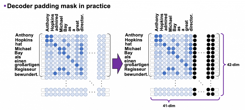
Decoder padding masks are almost the same as encoder one. You have to keep it in mind that you zero pad positions which surpassed the length of the source input sentence.

6 Decoding process

In the last section we have seen that we can zero-pad columns, but still the rows are redundant. However I guess that is not a big problem because you decode the final output in the direction of the rows of attention maps. Once you decode <end> token, you stop decoding. The redundant rows would not affect the decoding anymore.

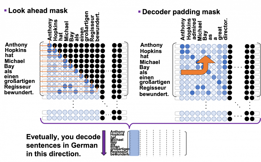
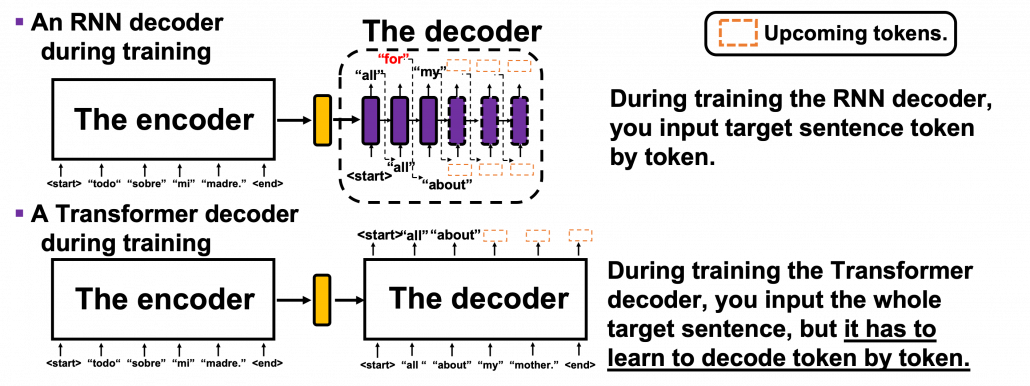
This decoding process is similar to that of seq2seq models with RNNs, and that is why you need to hide future tokens in the self-multi-head attention mechanism in the decoder. You share the same densely connected layers followed by a softmax function, at all the time steps of decoding. Transformer has to learn how to decode only based on the words which have appeared so far.

According to the original paper, “We also modify the self-attention sub-layer in the decoder stack to prevent positions from attending to subsequent positions. This masking, combined with fact that the output embeddings are offset by one position, ensures that the predictions for position $i$ can depend only on the known outputs at positions less than $i$ .” After these explanations, I think you understand the part more clearly.

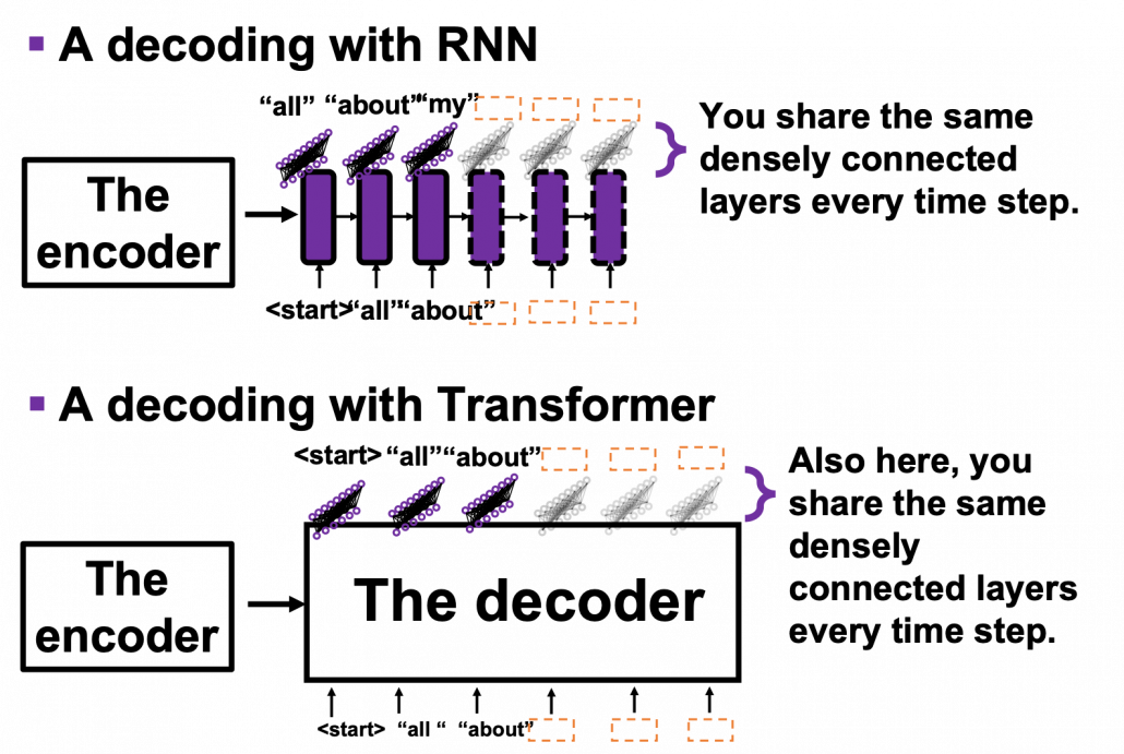
The codes blow is for the decoding part. You can see that you first start decoding an output sentence with a sentence composed of only <start>, and you decide which word to decoded, step by step.

*It easy to imagine that this decoding procedure is not the best. In reality you have to consider some possibilities of decoding, and you can do that with beam search decoding.

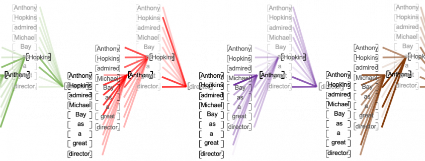
After training this English-German translator for 30 epochs you can translate relatively simple English sentences into German. I displayed some results below, with heat maps of multi-head attention. Each colored attention maps corresponds to each head of multi-head attention. The examples below are all from the fourth (last) layer, but you can visualize maps in any layers. When it comes to look ahead attention, naturally only the lower triangular part of the maps is activated.

This article series has not covered some important topics machine translation, for example how to calculate translation errors. Actually there are many other fascinating topics related to machine translation. For example beam search decoding, which consider some decoding possibilities, or other topics like how to handle proper nouns such as “Anthony” or “Hopkins.” But this article series is not on NLP. I hope you could effectively learn the architecture of Transformer model with examples of languages so far. And also I have not explained some details of training the network, but I will not cover that because I think that depends on tasks. The next article is going to be the last one of this series, and I hope you can see how Transformer is applied in computer vision fields, in a more “linguistic” manner.

But anyway we have finally made it. In this article series we have seen that one of the earliest computers was invented to break Enigma. And today we can quickly make a more or less accurate translator on our desk. With Transformer models, you can even translate deadly funny jokes into German.

*You can train a translator with this code.

*After training a translator, you can translate English sentences into German with this code.

[References]

[1] Ashish Vaswani, Noam Shazeer, Niki Parmar, Jakob Uszkoreit, Llion Jones, Aidan N. Gomez, Lukasz Kaiser, Illia Polosukhin, “Attention Is All You Need” (2017)

[2] “Transformer model for language understanding,” Tensorflow Core
https://www.tensorflow.org/overview

[3] Jay Alammar, “The Illustrated Transformer,”
http://jalammar.github.io/illustrated-transformer/

[4] “Stanford CS224N: NLP with Deep Learning | Winter 2019 | Lecture 14 – Transformers and Self-Attention,” stanfordonline, (2019)
https://www.youtube.com/watch?v=5vcj8kSwBCY

[5]Tsuboi Yuuta, Unno Yuuya, Suzuki Jun, “Machine Learning Professional Series: Natural Language Processing with Deep Learning,” (2017), pp. 91-94
坪井祐太、海野裕也、鈴木潤著, 「機械学習プロフェッショナルシリーズ深層学習による自然言語処理」, (2017), pp. 191-193

* I make study materials on machine learning, sponsored by DATANOMIQ. I do my best to make my content as straightforward but as precise as possible. I include all of my reference sources. If you notice any mistakes in my materials, including grammatical errors, please let me know (email: yasuto.tamura@datanomiq.de). And if you have any advice for making my materials more understandable to learners, I would appreciate hearing it.

Positional encoding, residual connections, padding masks: covering the rest of Transformer components

April 22, 2021/in Artificial Intelligence, Data Science, Data Science Hack, Deep Learning, Machine Learning, Main Category, Python, TensorFlow/by Yasuto Tamura

This is the fourth article of my article series named “Instructions on Transformer for people outside NLP field, but with examples of NLP.”

1 Wrapping points up so far

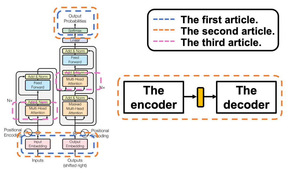
This article series has already covered a great deal of the Transformer mechanism. Whether you have read my former articles or not, I bet you are more or less lost in the course of learning Transformer model. The left side of the figure below is from the original paper on Transformer model, and my previous articles explained the parts in each colored frame. In the first article, I mainly explained how language is encoded in deep learning task and how that is evaluated.

This is more of a matter of inputs and the outputs of deep learning networks, which are in blue dotted frames in the figure. They are not so dependent on types of deep learning NLP tasks. In the second article, I explained seq2seq models, which are encoder-decoder models used in machine translation. Seq2seq models can can be simplified like the figure in the orange frame. In the article I mainly explained seq2seq models with RNNs, but the purpose of this article series is ultimately replace them with Transformer models. In the last article, I finally wrote about some actual components of Transformer models: multi-head attention mechanism. I think this mechanism is the core of Transformed models, and I did my best to explain it with a whole single article, with a lot of visualizations. However, there are still many elements I have not explained.

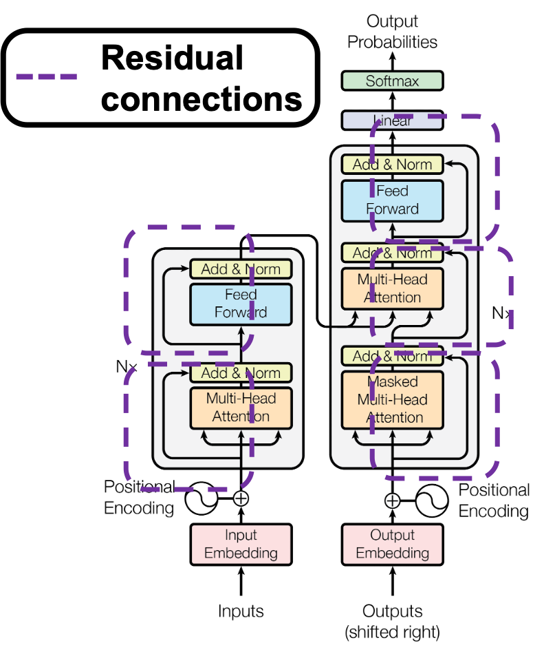
First, you need to do positional encoding to the word embedding so that Transformer models can learn the relations of the positions of input tokens. At least I was too stupid to understand what this is only with the original paper on Transformer. I am going to explain this algorithm in illustrative ways, which I needed to self-teach it. The second point is residual connections.

The last article has already explained multi-head attention, as precisely as I could do, but I still have to say I covered only two multi-head attention parts in a layer of Transformer model, which are in pink frames. During training, you have to mask some tokens at the decoder part so that some of tokens are invisible, and masked multi-head attention enables that.

You might be tired of the words “queries,” “keys,” and “values,” if you read the last article. But in fact that was not enough. When you think about applying Transformer in other tasks, such as object detection or image generation, you need to reconsider what the structure of data and how “queries,” “keys,” and “values,” correspond to each elements of the data, and probably one of my upcoming articles would cover this topic.

2 Why Transformer?

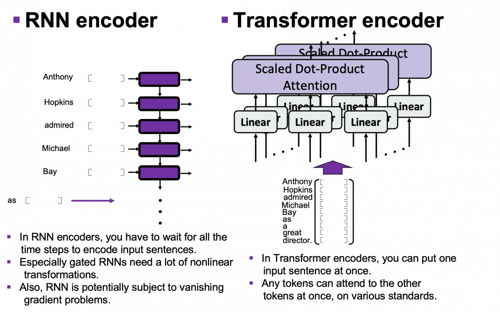
One powerful strength of Transformer model is its parallelization. As you saw in the last article, Trasformer models enable calculating relations of tokens to all other tokens, on different standards, independently in each head. And each head requires very simple linear transformations. In case of RNN encoders, if an input has $\tau$ tokens, basically you have to wait for $\tau$ time steps to finish encoding the input sentence. Also, at the time step $(\tau)$ the RNN cell retains the information at the time step $(1)$ only via recurrent connections. In this way you cannot attend to tokens in the earlier time steps, and this is obviously far from how we compare tokens in a sentence. You can bring information backward by bidirectional connection s in RNN models, but that all the more deteriorate parallelization of the model. And possessing information via recurrent connections, like a telephone game, potentially has risks of vanishing gradient problems. Gated RNN, such as LSTM or GRU mitigate the problems by a lot of nonlinear functions, but that adds to computational costs. If you understand multi-head attention mechanism, I think you can see that Transformer solves those problems.

I guess this is closer to when you speak a foreign language which you are fluent in. You wan to say something in a foreign language, and you put the original sentence in your mother tongue in the “encoder” in your brain. And you decode it, word by word, in the foreign language. You do not have to wait for the word at the end in your language, or rather you have to consider the relations of of a chunk of words to another chunk of words, in forward and backward ways. This is crucial especially when Japanese people speak English. You have to make the conclusion clear in English usually with the second word, but the conclusion is usually at the end of the sentence in Japanese.

3 Positional encoding

I explained disadvantages of RNN in the last section, but RNN has been a standard algorithm of neural machine translation. As I mentioned in the fourth section of the first article of my series on RNN, other neural nets like fully connected layers or convolutional neural networks cannot handle sequence data well. I would say RNN could be one of the only algorithms to handle sequence data, including natural language data, in more of classical methods of time series data processing.

*As I explained in this article, the original idea of RNN was first proposed in 1997, and I would say the way it factorizes time series data is very classical, and you would see similar procedures in many other algorithms. I think Transformer is a successful breakthrough which gave up the idea of processing sequence data time step by time step.

You might have noticed that multi-head attention mechanism does not explicitly uses the the information of the orders or position of input data, as it basically calculates only the products of matrices. In the case where the input is “Anthony Hopkins admired Michael Bay as a great director.”, multi head attention mechanism does not uses the information that “Hopkins” is the second token, or the information that the token two time steps later is “Michael.” Transformer tackles this problem with an almost magical algorithm named positional encoding.

In order to learn positional encoding, you should first think about what kind of encoding is ideal. According to this blog post, ideal encoding of positions of tokens have the following features.

Positional encoding of one token deterministically represents the position of the token.
The actual values of positional encoding should not be too big compared to the values of elements of embedding vectors.
Positional encodings of different tokens should successfully express their relative positions.

The most straightforward way to give the information of position is implementing the index of times steps $(t)$ , but if you naively give the term $(t)$ to the data, the term could get too big compared to the values of data ,for example when the sequence data is 100 time steps long. The next straightforward idea is compressing the idea of time steps to for example the range $[0, 1]$ . With this approach, however, the resolution of encodings can vary depending on the length of the input sequence data. Thus these naive approaches do not meet the requirements above, and I guess even conventional RNN-based models were not so successful in these points.

*I guess that is why attention mechanism of RNN seq2seq models, which I explained in the second article, was successful. You can constantly calculate the relative positions of decoder tokens compared to the encoder tokens.

Positional encoding, to me almost magically, meets the points I have mentioned. However the explanation of positional encoding in the original paper of Transformer is unkindly brief. It says you can encode positions of tokens with the following vector $PE_{(pos, 2i)} = sin(pos / 10000^{2i/d_model})$ , $PE_{(pos, 2i+1)} = cos(pos / 10000^{2i/d_model})$ , where $i = 0, 1, \dots, d_{model}/2 - 1$ . $d_{model}$ is the dimension of word embedding. The heat map below is the most typical type of visualization of positional encoding you would see everywhere, and in this case $d_{model}=256$ , and $pos$ is discrete number which varies from $0$ to $49$ , thus the heat map blow is equal to a $50\times 256$ matrix, whose elements are from $-1$ to $1$ . Each row of the graph corresponds to one token, and you can see that lower dimensional part is constantly changing like waves. Also it is quite easy to encode an input with this positional encoding: assume that you have a matrix of an input sentence composed of 50 tokens, each of which is a 256 dimensional vector, then all you have to do is just adding the heat map below to the matrix.

Concretely writing down, the encoding of the 256-dim token at $pos$ is $(PE_{(pos, 0)}, PE_{(pos, 1)}, \dots , PE_{(pos, 254)}, PE_{(pos, 255)})^T =$ $\bigl( sin(pos / 10000^{0/256}), cos(pos / 10000^{0/256}) \bigr), \dots , \bigl( sin(pos / 10000^{254/256}), cos(pos / 10000^{254/256}) \bigr)^T$ .

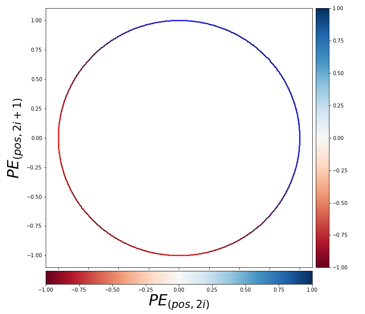
You should see this encoding more as $d_{model} / 2$ pairs of circles rather than $d_{model}$ dimensional vectors. When you fix the $i$ , the index of the depth of each encoding, you can extract a 2 dimensional vector $\boldsymbol{PE}_i =$ $\bigl( sin(pos / 10000^{2i/d_model}), cos(pos / 10000^{2i/d_model}) \bigr)$ . If you constantly change the value $pos$ , the vector $\boldsymbol{PE}_i$ rotates clockwise on the unit circle in the figure below.

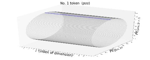
Also, the deeper the dimension of the embedding is, I mean the bigger the index $i$ is, the smaller the frequency of rotation is. I think the video below is a more intuitive way to see how each token is encoded with positional encoding. You can see that the bigger $pos$ is, that is the more tokens an input has, the deeper part positional encoding starts to rotate on the circles.

Very importantly, the original paper of Transformer says, “We chose this function because we hypothesized it would allow the model to easily learn to attend by relative positions, since for any fixed offset $k$ , $PE_{pos+k}$ can be represented as a linear function of $PE_{pos}$ .” For each circle at any depth, I mean for any $i$ , the following simple equation holds:

$\left( \begin{array}{c} sin(\frac{pos+k}{10000^{2i/d_{model}}}) \\ cos(\frac{pos+k}{10000^{2i/d_{model}}}) \end{array} \right) =$
$\left( \begin{array}{ccc} cos(\frac{k}{10000^{2i/d_{model}}}) & sin(\frac{k}{10000^{2i/d_{model}}}) \\ -sin(\frac{k}{10000^{2i/d_{model}}}) & cos(\frac{k}{10000^{2i/d_{model}}}) \\ \end{array} \right) \cdot \left( \begin{array}{c} sin(\frac{pos}{10000^{2i/d_{model}}}) \\ cos(\frac{pos}{10000^{2i/d_{model}}}) \end{array} \right)$

The matrix is a simple rotation matrix, so if $i$ is fixed the rotation only depends on $k$ , how many positions to move forward or backward. Then we get a very important fact: as the $pos$ changes ( $pos$ is a discrete number), each point rotates in proportion to the offset of “pos,” with different frequencies depending on the depth of the circles. The deeper the circle is, the smaller the frequency is. That means, this type of positional encoding encourages Transformer models to learn definite and relative positions of tokens with rotations of those circles, and the values of each element of the rotation matrices are from $-1$ to $1$ , so they do not get bigger no matter how many tokens inputs have.

For example when an input is “Anthony Hopkins admired Michael Bay as a great director.”, a shift from the token “Hopkins” to “Bay” is a rotation matrix $\left( \begin{array}{ccc} cos(\frac{k}{10000^{2i/d_{model}}}) & sin(\frac{k}{10000^{2i/d_{model}}}) \\ -sin(\frac{k}{10000^{2i/d_{model}}}) & cos(\frac{k}{10000^{2i/d_{model}}}) \\ \end{array} \right)$ , where $k=3$ . Also the shift from “Bay” to “great” has the same rotation.

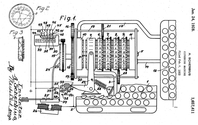
*Positional encoding reminded me of Enigma, a notorious cipher machine used by Nazi Germany. It maps alphabets to different alphabets with different rotating gear connected by cables. With constantly changing gears and keys, it changed countless patterns of alphabetical mappings, every day, which is impossible for humans to solve. One of the first form of computers was invented to break Enigma.

*As far as I could understand from “Imitation Game (2014).”

*But I would say Enigma only relied on discrete deterministic algebraic mapping of alphabets. The rotations of positional encoding is not that tricky as Enigma, but it can encode both definite and deterministic positions of much more variety of tokens. Or rather I would say AI algorithms developed enough to learn such encodings with subtle numerical changes, and I am sure development of NLP increased the possibility of breaking the Turing test in the future.

5 Residual connections

If you naively stack neural networks with simple implementation, that would suffer from vanishing gradient problems during training. Back propagation is basically multiplying many gradients, so

One way to mitigate vanishing gradient problems is quite easy: you have only to make a bypass of propagation. You would find a lot of good explanations on residual connections, so I am not going to explain how this is effective for vanishing gradient problems in this article.

In Transformer models you add positional encodings to the input only in the first layer, but I assume that the encodings remain through the layers by these bypass routes, and that might be one of reasons why Transformer models can retain information of positions of tokens.

6 Masked multi-head attention

Even though Transformer, unlike RNN, can attend to the whole input sentence at once, the decoding process of Transformer-based translator is close to RNN-based one, and you are going to see that more clearly in the codes in the next article. As I explained in the second article, RNN decoders decode each token only based on the tokens the have generated so far. Transformer decoder also predicts the output sequences autoregressively one token at a time step, just as RNN decoders. I think it easy to understand this process because RNN decoder generates tokens just as you connect RNN cells one after another, like connecting rings to a chain. In this way it is easy to make sure that generating of one token in only affected by the former tokens. On the other hand, during training Transformer decoders, you input the whole sentence at once. That means Transformer decoders can see the whole sentence during training. That is as if a student preparing for a French translation test could look at the whole answer French sentences. It is easy to imagine that you cannot prepare for the French test effectively if you study this way. Transformer decoders also have to learn to decode only based on the tokens they have generated so far.

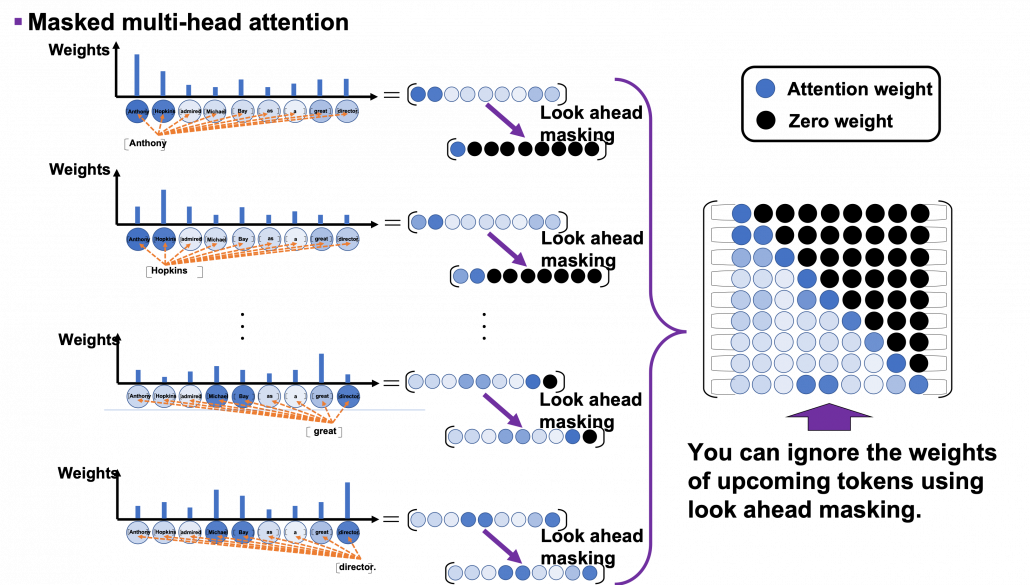
In order to properly train a Transformer-based translator to learn such decoding, you have to hide the upcoming tokens in target sentences during training. During calculating multi-head attentions in each Transformer layer, if you keep ignoring the weights from up coming tokens like in the figure below, it is likely that Transformer models learn to decode only based on the tokens generated so far. This is called masked multi-head attention.

*I am going to take an input “Anthonly Hopkins admire Michael Bay as a great director.” as an example of calculating masked multi-head attention mechanism, but this is supposed to be in the target laguage. So when you train an translator from English to German, in practice you have to calculate masked multi-head atetntion of “Anthony Hopkins hat Michael Bay als einen großartigen Regisseur bewundert.”

As you can see from the whole architecture of Transformer, you only need to consider masked multi-head attentions of of self-attentions of the input sentences at the decoder side. In order to concretely calculate masked multi-head attentions, you need a technique named look ahead masking. This is also quite simple. Just as well as the last article, let’s take an example of calculating self attentions of an input “Anthony Hopkins admired Michael Bay as a great director.” Also in this case you just calculate multi-head attention as usual, but when you get the histograms below, you apply look ahead masking to each histogram and delete the weights from the future tokens. In the figure below the black dots denote zero, and the sum of each row of the resulting attention map is also one. In other words, you get a lower triangular matrix, the sum of whose each row is 1.

Also just as I explained in the last article, you reweight vlaues with the triangular attention map. The figure below is calculating a transposed masked multi-head attention because I think it is a more straightforward way to see how vectors are reweighted in multi-head attention mechanism.

When you closely look at how each column of the transposed multi-head attention is reweighted, you can clearly see that the token is reweighted only based on the tokens generated so far.

*If you are still not sure why you need such masking in multi-head attention of target sentences, you should proceed to the next article for now. Once you check the decoding processes of Transformer-based translators, you would see why you need masked multi-head attention mechanism on the target sentence during training.

If you have read my articles, at least this one and the last one, I think you have gained more or less clear insights into how each component of Transfomer model works. You might have realized that each components require simple calculations. Combined with the fact that multi-head attention mechanism is highly parallelizable, Transformer is easier to train, compared to RNN.

In this article, we are going to see how masking of multi-head attention is implemented and how the whole Transformer structure is constructed. By the end of the next article, you would be able to create a toy English-German translator with more or less clear understanding on its architecture.

Appendix

You can visualize positional encoding the way I explained with simple Python codes below. Please just copy and paste them, importing necessary libraries. You can visualize positional encoding as both heat maps and points rotating on rings, and in this case the dimension of word embedding is 256, and the maximum length of sentences is 50.

# I borrowed this code from Tensorflow official tutorial.

# https://www.tensorflow.org/tutorials/text/transformer

import matplotlib as mpl

from mpl_toolkits.mplot3d import Axes3D

import numpy as np

import matplotlib.pyplot as plt

from matplotlib import cm

def get_angles(pos, i, d_model):

angle_rates = 1 / np.power(10000, (2 * (i//2)) / np.float32(d_model))

return pos * angle_rates

def positional_encoding(position, d_model):

angle_rads = get_angles(np.arange(position)[:, np.newaxis],

np.arange(d_model)[np.newaxis, :],

d_model)

# apply sin to even indices in the array; 2i

angle_rads[:, 0::2] = np.sin(angle_rads[:, 0::2])

# apply cos to odd indices in the array; 2i+1

angle_rads[:, 1::2] = np.cos(angle_rads[:, 1::2])

pos_encoding = angle_rads[np.newaxis, ...]

return pos_encoding.astype(np.float32)

resolution = 50

d_model = 256

n, d = resolution, d_model

pos_encoding = positional_encoding(n, d)

pos_encoding = pos_encoding[0]

plt.figure(figsize=(25, 10))

plt.pcolormesh(pos_encoding, cmap='RdBu')

plt.gca().invert_yaxis()

plt.ylabel('pos (the position of token)', fontsize=30)

plt.xlabel('$2i, 2i+1$', fontsize=30)

plt.colorbar()

plt.title("Positional encoding of 50 256-d tokens", fontsize=40)

plt.savefig("positional_encoding_heat_map.png")

plt.show()

import matplotlib as mpl

from mpl_toolkits.mplot3d import Axes3D

import numpy as np

import matplotlib.pyplot as plt

from matplotlib import cm

def get_angles(pos, i, d_model):

angle_rates = 1 / np.power(10000, (2 * (i//2)) / np.float32(d_model))

return pos * angle_rates

def positional_encoding(position, d_model):

angle_rads = get_angles(np.arange(position)[:, np.newaxis],

np.arange(d_model)[np.newaxis, :],

d_model)

# apply sin to even indices in the array; 2i

angle_rads[:, 0::2] = np.sin(angle_rads[:, 0::2])

# apply cos to odd indices in the array; 2i+1

angle_rads[:, 1::2] = np.cos(angle_rads[:, 1::2])

pos_encoding = angle_rads[np.newaxis, ...]

return pos_encoding.astype(np.float32)

# A function to mix blue and red colors.

def blue_red_gradation(x, y):

red = np.array([1.0, 0.0, 0.0])

blue = np.array([0.0, 0.0, 1.0])

combined_color_x = (max(0, x)*blue + abs(min(x, 0))*red)/(abs(x) + abs(y))

combined_color_y = (max(0, y)*blue + abs(min(y, 0))*red)/(abs(x) + abs(y))

combined_color = (combined_color_x*abs(x) + combined_color_y*abs(y))/(abs(x) + abs(y))

return combined_color[np.newaxis, ...]

resolution = 50

d_model = 256

x_range = 512

x_coordinates = np.linspace(0, d_model//2 - 1, d_model//2)

radius = 1

angular_velocity = np.pi / 12

y_coordinates = radius*np.cos(np.linspace(0, 1, resolution)*2*np.pi)

z_coordinates = radius*np.sin(np.linspace(0, 1, resolution)*2*np.pi)

n, d = resolution, d_model

pos_encoding = positional_encoding(n, d)

pos_encoding = pos_encoding[0]

#ax = fig.add_subplot(1, 1, 1, projection='3d')

color_vec = [[1., 0., 1.]]

markersize = 1

for j in range(resolution):

#for j in range(5):

fig = plt.figure(figsize=(25, 10))

ax = fig.gca(projection='3d')

for i in range(d_model//2):

ax.plot(x_coordinates[i]*np.ones(len(y_coordinates)), y_coordinates, z_coordinates, c='black', alpha=0.2)

for i in range(len(x_coordinates)):

ax.scatter(x_coordinates[i], radius*pos_encoding[:, 0::2][j, i], radius*pos_encoding[:, 1::2][j, i],

c=blue_red_gradation(pos_encoding[:, 0::2][j, i], pos_encoding[:, 1::2][j, i]), alpha=0.5, s=20)

ax.grid(False)

ax.set_title(r'No. {} token ($pos$)'.format(j+1), fontsize=40)

ax.set_xlabel(r"$i$ (index of dimension)", fontsize=40)

ax.set_ylabel(r'$PE_{(pos, 2i)}$', fontsize=40)

ax.set_zlabel(r'$PE_{(pos, 2i+1)}$', fontsize=40)

ax.set_xticks(np.arange(0, d_model//2, 10))

plt.subplots_adjust(left=0, right=1, bottom=0, top=1)

#plt.savefig('./positional_encoding_gif/{}.png'.format(j+1))

plt.show()

*In fact some implementations use different type of positional encoding, as you can see in the codes below. In this case, embedding vectors are roughly divided into two parts, and each part is encoded with different sine waves. I have been using a metaphor of rotating rings or gears in this article to explain positional encoding, but to be honest that is not necessarily true of all the types of Transformer implementation. Some papers compare different types of pairs of positional encoding. The most important point is, Transformer models is navigated to learn positions of tokens with certain types of mathematical patterns.

[References]

[1] Ashish Vaswani, Noam Shazeer, Niki Parmar, Jakob Uszkoreit, Llion Jones, Aidan N. Gomez, Lukasz Kaiser, Illia Polosukhin, “Attention Is All You Need” (2017)

[2] “Transformer model for language understanding,” Tensorflow Core
https://www.tensorflow.org/overview

[3] Jay Alammar, “The Illustrated Transformer,”
http://jalammar.github.io/illustrated-transformer/

[4] “Stanford CS224N: NLP with Deep Learning | Winter 2019 | Lecture 14 – Transformers and Self-Attention,” stanfordonline, (2019)
https://www.youtube.com/watch?v=5vcj8kSwBCY

[5]Harada Tatsuya, “Machine Learning Professional Series: Image Recognition,” (2017), pp. 191-193
原田達也著, 「機械学習プロフェッショナルシリーズ画像認識」, (2017), pp. 191-193

[6] Amirhossein Kazemnejad, “Transformer Architecture: The Positional Encoding
Let’s use sinusoidal functions to inject the order of words in our model”, Amirhossein Kazemnejad’s Blog, (2019)
https://kazemnejad.com/blog/transformer_architecture_positional_encoding/

[7] Nicolas Carion, Francisco Massa, Gabriel Synnaeve, Nicolas Usunier, Alexander Kirillov, Sergey Zagoruyko, “End-to-End Object Detection with Transformers,” (2020)

[8]中西啓、「【第5回】機械式暗号機の傑作～エニグマ登場～」、HH News & Reports, (2011)
https://www.hummingheads.co.jp/reports/series/ser01/110714.html

[9]中西啓、「【第6回】エニグマ解読～第2次世界大戦とコンピュータの誕生～」、HH News & Reports, (2011)

[10]Tsuboi Yuuta, Unno Yuuya, Suzuki Jun, “Machine Learning Professional Series: Natural Language Processing with Deep Learning,” (2017), pp. 91-94
坪井祐太、海野裕也、鈴木潤著, 「機械学習プロフェッショナルシリーズ深層学習による自然言語処理」, (2017), pp. 191-193

[11]”Stanford CS224N: NLP with Deep Learning | Winter 2019 | Lecture 8 – Translation, Seq2Seq, Attention”, stanfordonline, (2019)
https://www.youtube.com/watch?v=XXtpJxZBa2c

On the difficulty of language: prerequisites for NLP with deep learning

January 27, 2021/in Artificial Intelligence, Big Data, Data Mining, Data Science, Data Science Hack, Deep Learning, Machine Learning, Main Category, Natural Language Processing, Python, TensorFlow, Text Mining/by Yasuto Tamura

This is the first article of my article series “Instructions on Transformer for people outside NLP field, but with examples of NLP.”

1 Preface

This section is virtually just my essay on language. You can skip this if you want to get down on more technical topic.

As I do not study in natural language processing (NLP) field, I would not be able to provide that deep insight into this fast changing deep leaning field throughout my article series. However at least I do understand language is a difficult and profound field, not only in engineering but also in many other study fields. Some people might be feeling that technologies are eliminating languages, or one’s motivations to understand other cultures. First of all, I would like you to keep it in mind that I am not a geek who is trying to turn this multilingual world into a homogeneous one and rebuild Tower of Babel, with deep learning. I would say I am more keen on social or anthropological sides of language.

I think you would think more about languages if you have mastered at least one foreign language. As my mother tongue is Japanese, which is totally different from many other Western languages in terms of characters and ambiguity, I understand translating is not what learning a language is all about. Each language has unique characteristics, and I believe they more or less influence one’s personalities. For example, many Western languages make the verb, I mean the conclusion, of sentences clear in the beginning part of the sentences. That is also true of Chinese, I heard. However in Japanese, the conclusion comes at the end, so that is likely to give an impression that Japanese people are being obscure or indecisive. Also, Japanese sentences usually omit their subjects. In German as well, the conclusion of a sentences tend to come at the end, but I am almost 100% sure that no Japanese people would feel German people make things unclear. I think that comes from the structures of German language, which tends to make the number, verb, relations of words crystal clear.

Source: https://twitter.com/nakamurakihiro

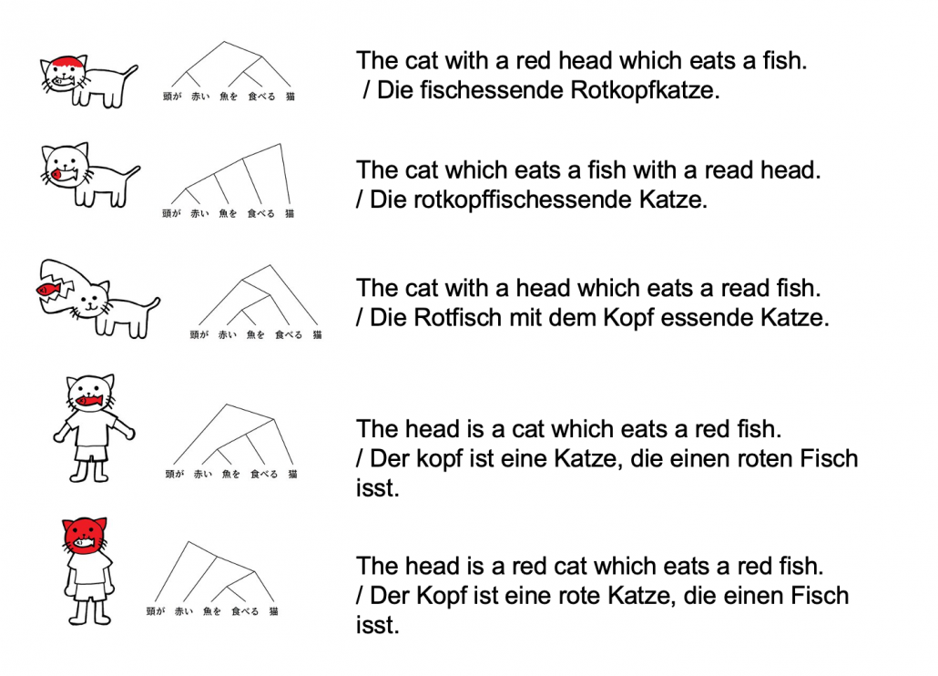
Let’s take an example to see how obscure Japanese is. A Japanese sentence 「頭が赤い魚を食べる猫」can be interpreted in five ways, depending on where you put emphases on.

Common sense tells you that the sentence is likely to mean the first two cases, but I am sure they can mean those five possibilities. There might be similarly obscure sentences in other languages, but I bet few languages can be as obscure as Japanese. Also as you can see from the last two sentences, you can omit subjects in Japanese. This rule is nothing exceptional. Japanese people usually don’t use subjects in normal conversations. And when you read classical Japanese, which Japanese high school students have to do just like Western students learn some of classical Latin, the writings omit subjects much more frequently.

*However interestingly we have rich vocabulary of subjects. The subject “I” can be translated to 「私」、「僕」、「俺」、「自分」、「うち」etc, depending on your personality, who you are talking to, and the time when it is written in.

I believe one can see the world only in the framework of their language, and it seems one’s personality changes depending on the language they use. I am not sure whether the language originally determines how they think, or how they think forms the language. But at least I would like you to keep it in mind that if you translate a conversation, for example a random conversation at a bar in Berlin, into Japanese, that would linguistically sound Japanese, but not anthropologically. Imagine that such kind of random conversation in Berlin or something is like playing a catch, I mean throwing a ball named “your opinion.” On the other hand, normal conversations of Japanese people are in stead more of, I would say, “resonance” of several tuning forks. They do their bests to show that they are listening to each other, by excessively nodding or just repeating “Really?”, but usually it seems hardly any constructive dialogues have been made.

*I sometimes feel you do not even need deep learning to simulate most of such Japanese conversations. Several-line Python codes would be enough.

My point is, this article series is mainly going to cover only a few techniques of NLP in deep learning field: sequence to sequence model (seq2seq model) , and especially Transformer. They are, at least for now, just mathematical models and mappings of a small part of this profound field of language (as far as I can cover in this article series). But still, examples of language would definitely help you understand Transformer model in the long run.

2 Tokens and word embedding

*Throughout my article series, “words” just means the normal words you use in daily life. “Tokens” means more general unit of NLP tasks. For example the word “Transformer” might be denoted as a single token “Transformer,” or maybe as a combination of two tokens “Trans” and “former.”

One challenging part of handling language data is its encodings. If you started learning programming in a language other than English, you would have encountered some troubles of using keyboards with different arrangements or with characters. Some comments on your codes in your native languages are sometimes not readable on some software. You can easily get away with that by using only English, but when it comes to NLP you have to deal with this difficulty seriously. How to encode characters in each language should be a first obstacle of NLP. In this article we are going to rely on a library named BPEmb, which provides word embedding in various languages, and you do not have to care so much about encodings in languages all over the world with this library.

In the first section, you might have noticed that Japanese sentence is not separated with spaces like Western languages. This is also true of Chinese language, and that means we need additional tasks of separating those sentences at least into proper chunks of words. This is not only a matter of engineering, but also of some linguistic fields. Also I think many people are not so conscious of how sentences in their native languages are grammatically separated.

The next point is, unlike other scientific data, such as temperature, velocity, voltage, or air pressure, language itself is not measured as numerical data. Thus in order to process language, including English, you first have to map language to certain numerical data, and after some processes you need to conversely map the output numerical data into language data. This section is going to be mainly about one-hot encoding and word embedding, the ways to convert word/token into numerical data. You might already have heard about this

You might have learnt about word embedding to some extent, but I hope you could get richer insight into this topic through this article.

2.1 One-hot encoding

One-hot encoding would be the most straightforward way to encode words/tokens. Assume that you have a dictionary whose size is $|\mathcal{V}|$ , and it includes words from “a”, “ablation”, “actually” to “zombie”, “?”, “!”

In a mathematical manner, in order to choose a word out of those $|\mathcal{V}|$ words, all you need is a $|\mathcal{V}|$ dimensional vector, one of whose elements is $1$ , and the others are $0$ . When you want to choose the No. i word, which is “indeed” in the example below, its corresponding one-hot vector is $\boldsymbol{v} = (0, \dots, 1, \dots, 0 )$ , where only the No. i element is $1$ . One-hot encoding is also easy to understand, and that’s all. It is easy to imagine that people have already come up with more complicated and better way to encoder words. And one major way to do that is word embedding.

2.2 Word embedding

Source: Francois Chollet, Deep Learning with Python,(2018), Manning

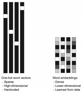
Actually word embedding is related to one-hot encoding, and if you understand how to train a simple neural network, for example densely connected layers, you would understand word embedding easily. The key idea of word embedding is denoting each token with a $D$ dimensional vector, whose dimension is fewer than the vocabulary size $|\mathcal{V}|$ . The elements of the resulting word embedding vector are real values, I mean not only 0 or 1. Obviously you can encode much richer variety of tokens with such vectors. The figure at the left side is from “Deep Learning with Python” by François Chollet, and I think this is an almost perfect and simple explanation of the comparison of one-hot encoding and word embedding. But the problem is how to get such convenient vectors. The answer is very simple: you have only to train a network whose inputs are one-hot vector of the vocabulary.

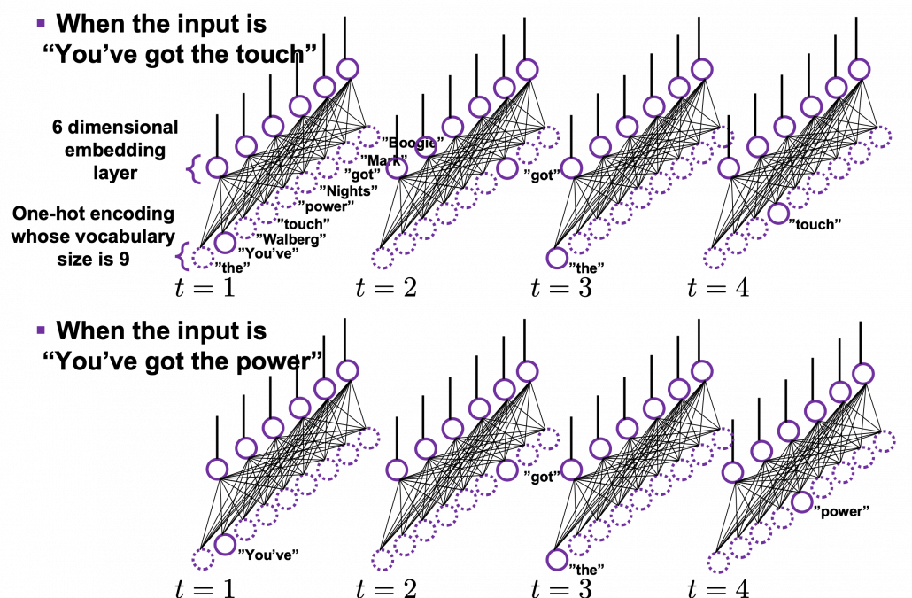
The figure below is a simplified model of word embedding of a certain word. When the word is input into a neural network, only the corresponding element of the one-hot vector is 1, and that virtually means the very first input layer is composed of one neuron whose value is 1. And the only one neuron propagates to the next D dimensional embedding layer. These weights are the very values which most other study materials call “an embedding vector.”

When you input each word into a certain network, for example RNN or Transformer, you map the input one-hot vector into the embedding layer/vector. The examples in the figure are how inputs are made when the input sentences are “You’ve got the touch” and “You’ve got the power.” Assume that you have a dictionary of one-hot encoding, whose vocabulary is {“the”, “You’ve”, “Walberg”, “touch”, “power”, “Nights”, “got”, “Mark”, “Boogie”}, and the dimension of word embeding is 6. In this case $|\mathcal{V}| = 9, D=6$ . When the inputs are “You’ve got the touch” or “You’ve got the power” , you put the one-hot vector corresponding to “You’ve”, “got”, “the”, “touch” or “You’ve”, “got”, “the”, “power” sequentially every time step $t$ .

In order to get word embedding of certain vocabulary, you just need to train the network. We know that the words “actually” and “indeed” are used in similar ways in writings. Thus when we propagate those words into the embedding layer, we can expect that those embedding layers are similar. This is how we can mathematically get effective word embedding of certain vocabulary.

More interestingly, if word embedding is properly trained, you can mathematically “calculate” words. For example, $\boldsymbol{v}_{king} - \boldsymbol{v}_{man} + \boldsymbol{v}_{woman} \approx \boldsymbol{v}_{queen}$ , $\boldsymbol{v}_{Japan} - \boldsymbol{v}_{Tokyo} + \boldsymbol{v}_{Vietnam} \approx \boldsymbol{v}_{Hanoi}$ .

*I have tried to demonstrate this type of calculation on several word embedding, but none of them seem to work well. At least you should keep it in mind that word embedding learns complicated linear relations between words.

I should explain word embedding techniques such as word2vec in detail, but the main focus of this article is not NLP, so the points I have mentioned are enough to understand Transformer model with NLP examples in the upcoming articles.

3 Language model

Language models is one of the most straightforward, but crucial ideas in NLP. This is also a big topic, so this article is going to cover only basic points. Language model is a mathematical model of the probabilities of which words to come next, given a context. For example if you have a sentence “In the lecture, he opened a _.”, a language model predicts what comes at the part “_.” It is obvious that this is contextual. If you are talking about general university students, “_” would be “textbook,” but if you are talking about Japanese universities, especially in liberal art department, “_” would be more likely to be “smartphone. I think most of you use this language model everyday. When you type in something on your computer or smartphone, you would constantly see text predictions, or they might even correct your spelling or grammatical errors. This is language modelling. You can make language models in several ways, such as n-gram and neural language models, but in this article I can explain only general formulations for such models.

*I am not sure which algorithm is used in which services. That must be too fast changing and competitive for me to catch up.

As I mentioned in the first article series on RNN, a sentence is usually processed as sequence data in NLP. One single sentence is denoted as $\boldsymbol{X} = (\boldsymbol{x}^{(1)}, \dots, \boldsymbol{x}^{(\tau)})$ , a list of vectors. The vectors are usually embedding vectors, and the $(t)$ is the index of the order of tokens. For example the sentence “You’ve go the power.” can be expressed as $\boldsymbol{X} = (\boldsymbol{x}^{(1)}, \boldsymbol{x}^{(2)}, \boldsymbol{x}^{(3)}, \boldsymbol{x}^{(4)})$ , where $\boldsymbol{x}^{(1)}, \boldsymbol{x}^{(2)}, \boldsymbol{x}^{(3)}, \boldsymbol{x}^{(4)}$ denote “You’ve”, “got”, “the”, “power”, “.” respectively. In this case $\tau = 4$ .

In practice a sentence $\boldsymbol{X}$ usually includes two tokens $BOS$ and $EOS$ at the beginning and the end of the sentence. They mean “Beginning Of Sentence” and “End Of Sentence” respectively. Thus in many cases $\boldsymbol{X} = (\boldsymbol{BOS} , \boldsymbol{x}^{(1)}, \dots, \boldsymbol{x}^{(\tau)}, \boldsymbol{EOS} )$ . $\boldsymbol{BOS}$ and $\boldsymbol{EOS}$ are also both vectors, at least in the Tensorflow tutorial.

$P(\boldsymbol{X} =$ $(\boldsymbol{BOS}, \boldsymbol{x}^{(1)}, \dots, \boldsymbol{x}^{(\tau)}, \boldsymbol{EOS})$ is the probability of incidence of the sentence. But it is easy to imagine that it would be very hard to directly calculate how likely the sentence $\boldsymbol{X}$ appears out of all possible sentences. I would rather say it is impossible. Thus instead in NLP we calculate the probability $P(\boldsymbol{X})$ as a product of the probability of incidence or a certain word, given all the words so far. When you’ve got the words $(\boldsymbol{x}^{(1)}, \dots, \boldsymbol{x}^{(t-1})$ so far, the probability of the incidence of $\boldsymbol{x}^{(t)}$ , given the context is $P(\boldsymbol{x}^{(t)}|\boldsymbol{x}^{(1)}, \dots, \boldsymbol{x}^{(t-1)})$ . $P(\boldsymbol{BOS})$ is a probability of the the sentence $\boldsymbol{X}$ being $(\boldsymbol{BOS})$ , and the probability of $\boldsymbol{X}$ being $(\boldsymbol{BOS}, \boldsymbol{x}^{(1)})$ can be decomposed this way: $P(\boldsymbol{BOS}, \boldsymbol{x}^{(1)}) =$ $P(\boldsymbol{x}^{(1)}|\boldsymbol{BOS})P(\boldsymbol{BOS})$ .

Just as well $P(\boldsymbol{BOS}, \boldsymbol{x}^{(1)}, \boldsymbol{x}^{(2)}) =$ $P(\boldsymbol{x}^{(2)}| \boldsymbol{BOS}, \boldsymbol{x}^{(1)}) P( \boldsymbol{BOS}, \boldsymbol{x}^{(1)})=$ $P(\boldsymbol{x}^{(2)}| \boldsymbol{BOS}, \boldsymbol{x}^{(1)}) P(\boldsymbol{x}^{(1)}| \boldsymbol{BOS}) P( \boldsymbol{BOS})$ .

Hence, the general probability of incidence of a sentence $\boldsymbol{X}$ is $P(\boldsymbol{X})=P(\boldsymbol{BOS}, \boldsymbol{x}^{(1)}, \boldsymbol{x}^{(2)}, \dots, \boldsymbol{x}^{(\tau -1)}, \boldsymbol{x}^{(\tau)}, \boldsymbol{EOS}) =$ $P(\boldsymbol{EOS}| \boldsymbol{BOS}, \boldsymbol{x}^{(1)}, \dots, \boldsymbol{x}^{(\tau)})$ $P(\boldsymbol{x}^{(\tau)}| \boldsymbol{BOS}, \boldsymbol{x}^{(1)}, \dots, \boldsymbol{x}^{(\tau - 1)})$ $\cdots$ $P(\boldsymbol{x}^{(2)}| \boldsymbol{BOS}, \boldsymbol{x}^{(1)})$ $P(\boldsymbol{x}^{(1)}| \boldsymbol{BOS})$ $P(\boldsymbol{BOS})$ .

Let $\boldsymbol{x}^{(0)}$ be $\boldsymbol{BOS}$ and $\boldsymbol{x}^{(\tau + 1)}$ be $\boldsymbol{EOS}$ . Plus, let $P(\boldsymbol{x}^{(t+1)}|\boldsymbol{X}_{[0, t]})$ be $P(\boldsymbol{x}^{(t+1)}|\boldsymbol{x}^{(0)}, \dots, \boldsymbol{x}^{(t)})$ , then $P(\boldsymbol{X}) = P(\boldsymbol{x}^{(0)})\prod_{t=0}^{\tau}{P(\boldsymbol{x}^{(t+1)}|\boldsymbol{X}_{[0, t]})}$ . Language models calculate which words to come sequentially in this way.

Here’s a question: how would you evaluate a language model?

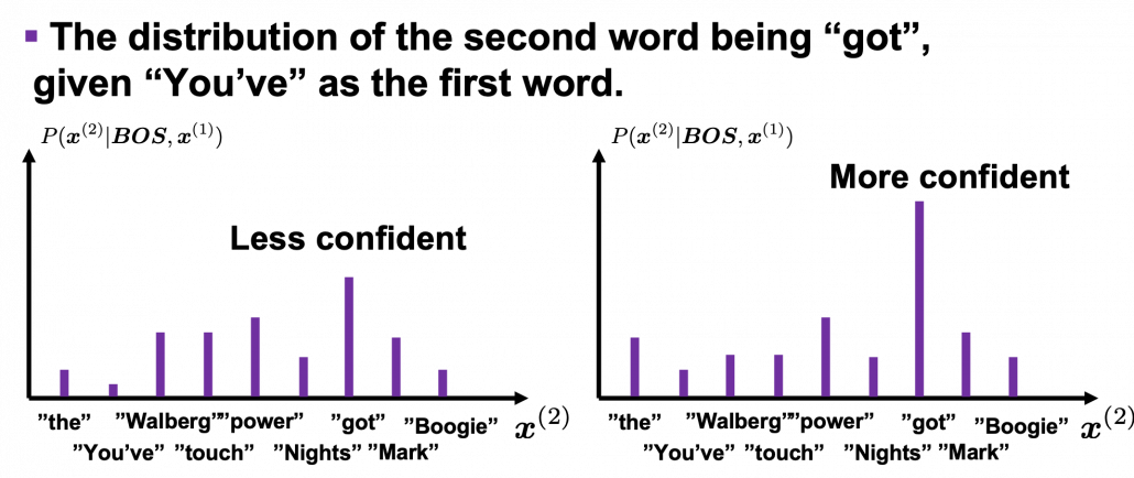
I would say the answer is, when the language model generates words, the more confident the language model is, the better the language model is. Given a context, when the distribution of the next word is concentrated on a certain word, we can say the language model is confident about which word to come next, given the context.

*For some people, it would be more understandable to call this “entropy.”

Let’s take the vocabulary {“the”, “You’ve”, “Walberg”, “touch”, “power”, “Nights”, “got”, “Mark”, “Boogie”} as an example. Assume that $P(\boldsymbol{X}) =$ $P(\boldsymbol{BOS}, \boldsymbol{You've}, \boldsymbol{got}, \boldsymbol{the}, \boldsymbol{touch}, \boldsymbol{EOS}) =$ $P(\boldsymbol{BOS}, \boldsymbol{x}^{(1)}, \boldsymbol{x}^{(2)}, \boldsymbol{x}^{(3)}, \boldsymbol{x}^{(4)}, \boldsymbol{EOS})=$ $P(\boldsymbol{x}^{(0)})\prod_{t=0}^{4}{P(\boldsymbol{x}^{(t+1)}|\boldsymbol{X}_{[0, t]})}$ . Given a context $(\boldsymbol{BOS}, \boldsymbol{x}^{(1)})$ , the probability of incidence of $\boldsymbol{x}^{(2)}$ is $P(\boldsymbol{x}^{2}|\boldsymbol{BOS}, \boldsymbol{x}^{(1)})$ . In the figure below, the distribution at the left side is less confident because probabilities do not spread widely, on the other hand the one at the right side is more confident that next word is “got” because the distribution concentrates on “got”.

*You have to keep it in mind that the sum of all possible probability $P(\boldsymbol{x}^{(2)} | \boldsymbol{BOS}, \boldsymbol{x}^{(1)})$ is $1$ , that is, $P(\boldsymbol{the}| \boldsymbol{BOS}, \boldsymbol{x}^{(1)}) +$ $P(\boldsymbol{You've}| \boldsymbol{BOS}, \boldsymbol{x}^{(1)}) + \cdots$ $+ P(\boldsymbol{Boogie}| \boldsymbol{BOS}, \boldsymbol{x}^{(1)}) = 1$ .

While the language model generating the sentence “BOS You’ve got the touch EOS”, it is better if the language model keeps being confident. If it is confident, $P(\boldsymbol{X})=$ $P(\boldsymbol{BOS})$ $P(\boldsymbol{x}^{(1)}|\boldsymbol{BOS}}P(\boldsymbol{x}^{(3)}|\boldsymbol{BOS}, \boldsymbol{x}^{(1)}, \boldsymbol{x}^{(2)})$ $P(\boldsymbol{x}^{(4)}|\boldsymbol{BOS}, \boldsymbol{x}^{(1)}, \boldsymbol{x}^{(2)}, \boldsymbol{x}^{(3)})$ $P(\boldsymbol{EOS}|\boldsymbol{BOS}, \boldsymbol{x}^{(1)}, \boldsymbol{x}^{(2)}, \boldsymbol{x}^{(3)}, \boldsymbol{x}^{(4)})}$ gets higher. Thus $(-1) \{ log_{b}{P(\boldsymbol{BOS})} +$ $log_{b}{P(\boldsymbol{x}^{(1)}|\boldsymbol{BOS}}) +$ $log_{b}{P(\boldsymbol{x}^{(3)}|\boldsymbol{BOS}, \boldsymbol{x}^{(1)}, \boldsymbol{x}^{(2)})} +$ $log_{b}{P(\boldsymbol{x}^{(4)}|\boldsymbol{BOS}, \boldsymbol{x}^{(1)}, \boldsymbol{x}^{(2)}, \boldsymbol{x}^{(3)})} +$ $log_{b}{P(\boldsymbol{EOS}|\boldsymbol{BOS}, \boldsymbol{x}^{(1)}, \boldsymbol{x}^{(2)}, \boldsymbol{x}^{(3)}, \boldsymbol{x}^{(4)})} \}$ gets lower, where usually $b=2$ or $b=e$ .

This is how to measure how confident language models are, and the indicator of the confidence is called perplexity. Assume that you have a data set for evaluation $\mathcal{D} = (\boldsymbol{X}_1, \dots, \boldsymbol{X}_n, \dots, \boldsymbol{X}_{|\mathcal{D}|})$ , which is composed of $|\mathcal{D}|$ sentences in total. Each sentence $\boldsymbol{X}_n =$ $(\boldsymbol{x}^{(0)})\prod_{t=0}^{\tau ^{(n)}}{P(\boldsymbol{x}_{n}^{(t+1)}|\boldsymbol{X}_{n, [0, t]})}$ has $\tau^{(n)}$ tokens in total excluding $\boldsymbol{BOS}, \boldsymbol{EOS}$ . And let $|\mathcal{V}|$ be the size of the vocabulary of the language model. Then the perplexity of the language model is $b^z$ , where $z = \frac{-1}{|\mathcal{V}|}\sum_{n=1}^{|\mathcal{D}|}{\sum_{t=0}^{\tau ^{(n)}}{log_{b}P(\boldsymbol{x}_{n}^{(t+1)}|\boldsymbol{X}_{n, [0, t]})}$ . The $b$ is usually $2$ or $e$ .

For example, assume that $\mathcal{V}$ is vocabulary {“the”, “You’ve”, “Walberg”, “touch”, “power”, “Nights”, “got”, “Mark”, “Boogie”}. Also assume that the evaluation data set for perplexity of a language model is $\mathcal{D} = (\boldsymbol{X}_1, \boldsymbol{X}_2)$ , where $\boldsymbol{X_1} =(\boldsymbol{You've}, \boldsymbol{got}, \boldsymbol{the}, \boldsymbol{touch})$ $\boldsymbol{X_2} = (\boldsymbol{You've}, \boldsymbol{got}, \boldsymbol{the }, \boldsymbol{power})$ . In this case $|\mathcal{V}|=9,$ $|\mathcal{D}|=2$ . I have already showed you how to calculate the perplexity of the sentence “You’ve got the touch.” above. You just need to do a similar thing on another sentence “You’ve got the power”, and then you can get the perplexity of the language model.

*If the network is not properly trained, it would also be confident of generating wrong outputs. However, such network still would give high perplexity because it is “confident” at any rate. I’m sorry I don’t know how to tackle the problem. Please let me put this aside, and let’s get down on Transformer model soon.

Appendix

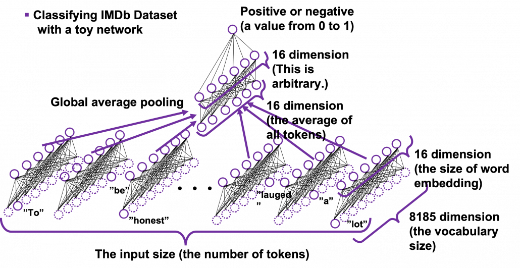
Let’s see how word embedding is implemented with a very simple example in the official Tensorflow tutorial. It is a simple binary classification task on IMDb Dataset. The dataset is composed to comments on movies by movie critics, and you have only to classify if the commentary is positive or negative about the movie. For example when you get you get an input “To be honest, Michael Bay is a terrible as an action film maker. You cannot understand what is going on during combat scenes, and his movies rely too much on advertisements. I got a headache when Mark Walberg used a Chinese cridit card in Texas. However he is very competent when it comes to humorous scenes. He is very talented as a comedy director, and I have to admit I laughed a lot.“, the neural netowork has to judge whether the statement is positive or negative.

This networks just takes an average of input embedding vectors and regress it into a one dimensional value from 0 to 1. The shape of embedding layer is (8185, 16). Weights of neural netowrks are usually implemented as matrices, and you can see that each row of the matrix corresponds to emmbedding vector of each token.

*It is easy to imagine that this technique is problematic. This network virtually taking a mean of input embedding vectors. That could mean if the input sentence includes relatively many tokens with negative meanings, it is inclined to be classified as negative. But for example, if the sentence is “This masterpiece is a dark comedy by Charlie Chaplin which depicted stupidity of the evil tyrant gaining power in the time. It thoroughly mocked Germany in the time as an absurd group of fanatics, but such propaganda could have never been made until ‘Casablanca.'” , this can be classified as negative, because only the part “masterpiece” is positive as a token, and there are much more words with negative meanings themselves.

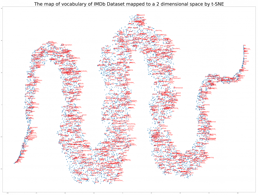
The official Tensorflow tutorial provides visualization of word embedding with Embedding Projector, but I would like you to take more control over the data by yourself. Please just copy and paste the codes below, installing necessary libraries. You would get a map of vocabulary used in the text classification task. It seems you cannot find clear tendency of the clusters of the tokens. You can try other dimension reduction methods to get maps of the vocabulary by for example using Scikit Learn.

import tensorflow as tf

from tensorflow import keras

from tensorflow.keras import layers

import tensorflow_datasets as tfds

tfds.disable_progress_bar()

(train_data, test_data), info = tfds.load(

'imdb_reviews/subwords8k',

split = (tfds.Split.TRAIN, tfds.Split.TEST),

with_info=True, as_supervised=True)

train_batches = train_data.shuffle(1000).padded_batch(10)

test_batches = test_data.shuffle(1000).padded_batch(10)

embedding_dim=16

encoder = info.features['text'].encoder

model = keras.Sequential([

layers.Embedding(encoder.vocab_size, embedding_dim),

layers.GlobalAveragePooling1D(),

layers.Dense(16, activation='relu'),

layers.Dense(1)

])

print("\n\nThe size of the vocabulary generated from IMDb Dataset is " + str(encoder.vocab_size) + '\n\n')

model.summary()

model.compile(optimizer='adam',

loss=tf.keras.losses.BinaryCrossentropy(from_logits=True),

metrics=['accuracy'])

history = model.fit(

train_batches,

epochs=10,

validation_data=test_batches, validation_steps=20)

word_embedding_vectors = model.layers[0].get_weights()[0]

print("\n\nThe shape of the trained weigths of the embedding layer is " + str(word_embedding_vectors.shape) + '\n\n')

from sklearn.manifold import TSNE

X_reduced = TSNE(n_components = 2, init='pca', random_state=0).fit_transform(word_embedding_vectors)

import numpy as np

embedding_dict = zip(encoder.subwords, np.arange(len(encoder.subwords)))

embedding_dict = dict(embedding_dict)

import matplotlib.pyplot as plt

plt.figure(figsize=(60, 45))

plt.scatter(X_reduced[:, 0], X_reduced[:, 1])

for i in range(0, len(encoder.subwords), 5):

plt.text(X_reduced[i, 0], X_reduced[i, 1], encoder.subwords[i], fontsize=20, color='red')

plt.title("The map of vocabulary of IMDb Dataset mapped to a 2 dimensional space by t-SNE", fontsize=60)

#plt.savefig('imdb_tsne_map.png')

plt.show()

[References]

[1] “Word embeddings” Tensorflow Core
https://www.tensorflow.org/tutorials/text/word_embeddings

[2]Tsuboi Yuuta, Unno Yuuya, Suzuki Jun, “Machine Learning Professional Series: Natural Language Processing with Deep Learning,” (2017), pp. 43-64, 72-85, 91-94
坪井祐太、海野裕也、鈴木潤著, 「機械学習プロフェッショナルシリーズ深層学習による自然言語処理」, (2017), pp. 43-64, 72-85, 191-193

[3]”Stanford CS224N: NLP with Deep Learning | Winter 2019 | Lecture 8 – Translation, Seq2Seq, Attention”, stanfordonline, (2019)
https://www.youtube.com/watch?v=XXtpJxZBa2c

[4] Francois Chollet, Deep Learning with Python,(2018), Manning , pp. 178-185

[5]”2.2. Manifold learning,” scikit-learn
https://scikit-learn.org/stable/modules/manifold.html

A brief history of neural nets: everything you should know before learning LSTM

July 16, 2020/in Artificial Intelligence, Data Mining, Data Science, Data Science Hack, Deep Learning, Machine Learning, Main Category, Predictive Analytics, TensorFlow/by Yasuto Tamura

This series is not a college course or something on deep learning with strict deadlines for assignments, so let’s take a detour from practical stuff and take a brief look at the history of neural networks.

The history of neural networks is also a big topic, which could be so long that I had to prepare another article series. And usually I am supposed to begin such articles with something like “The term ‘AI’ was first used by John McCarthy in Dartmouth conference 1956…” but you can find many of such texts written by people with much more experiences in this field. Therefore I am going to write this article from my point of view, as an intern writing articles on RNN, as a movie buff, and as one of many Japanese men who spent a great deal of childhood with video games.

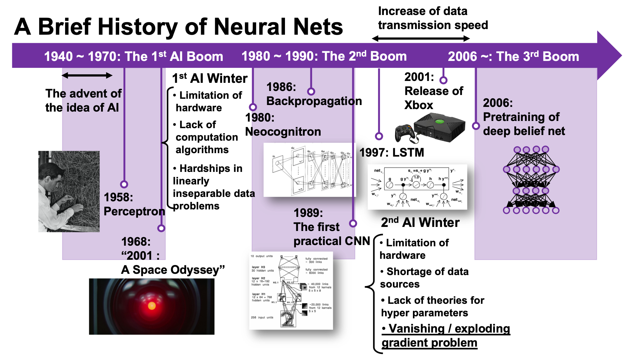
We are now in the third AI boom, and some researchers say this boom began in 2006. A professor in my university said there we are now in a kind of bubble economy in machine learning/data science industry, but people used to say “Stop daydreaming” to AI researchers. The second AI winter is partly due to vanishing/exploding gradient problem of deep learning. And LSTM was invented as one way to tackle such problems, in 1997.

1, First AI boom

In the first AI boom, I think people were literally “daydreaming.” Even though the applications of machine learning algorithms were limited to simple tasks like playing chess, checker, or searching route of 2d mazes, and sometimes this time is called GOFAI (Good Old Fashioned AI).

Source: https://www.youtube.com/watch?v=K-HfpsHPmvw&feature=youtu.be

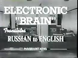
Even today when someone use the term “AI” merely for tasks with neural networks, that amuses me because for me deep learning is just statistically and automatically training neural networks, which are capable of universal approximation, into some classifiers/regressors. Actually the algorithms behind that is quite impressive, but the structure of human brains is much more complicated. The hype of “AI” already started in this first AI boom. Let me take an example of machine translation in this video. In fact the research of machine translation already started in the early 1950s, and of specific interest in the time was translation between English and Russian due to Cold War. In the first article of this series, I said one of the most famous applications of RNN is machine translation, such as Google Translation, DeepL. They are a type of machine translation called neural machine translation because they use neural networks, especially RNNs. Neural machine translation was an astonishing breakthrough around 2014 in machine translation field. The former major type of machine translation was statistical machine translation, based on statistical language models. And the machine translator in the first AI boom was rule base machine translators, which are more primitive than statistical ones.

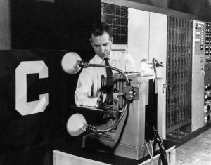
Source: https://news.cornell.edu/stories/2019/09/professors-perceptron-paved-way-ai-60-years-too-soon

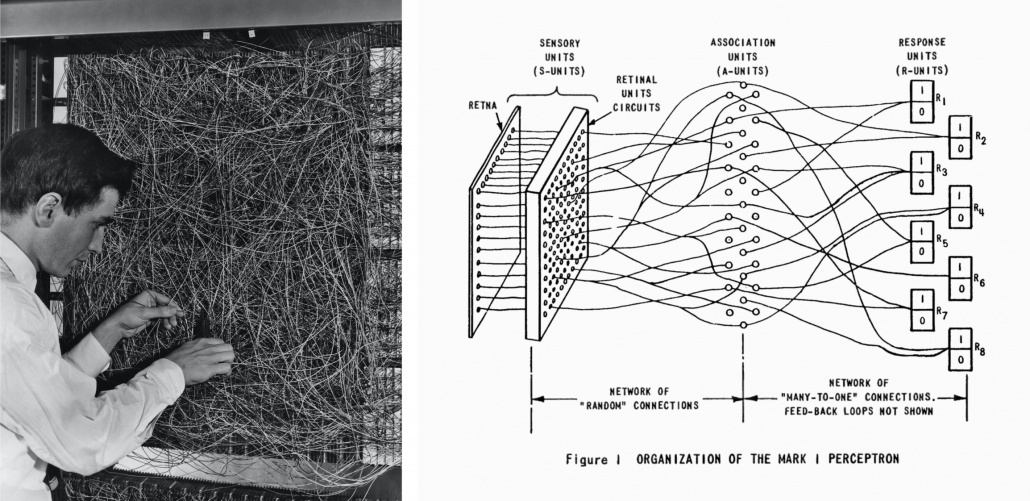
The most remarkable invention in this time was of course perceptron by Frank Rosenblatt. Some people say that this is the first neural network. Even though you can implement perceptron with a-few-line codes in Python, obviously they did not have Jupyter Notebook in those days. The perceptron was implemented as a huge instrument named Mark 1 Perceptron, and it was composed of randomly connected wires. I do not precisely know how it works, but it was a huge effort to implement even the most primitive type of neural networks. They needed to use a big lighting fixture to get a 20*20 pixel image using 20*20 array of cadmium sulphide photocells. The research by Rosenblatt, however, was criticized by Marvin Minsky in his book because perceptrons could only be used for linearly separable data. To make matters worse the criticism prevailed as that more general, multi-layer perceptrons were also not useful for linearly inseparable data (as I mentioned in the first article, multi-layer perceptrons, namely normal neural networks, can be universal approximators, which have potentials to classify/regress various types of complex data). In case you do not know what “linearly separable” means, imagine that there are data plotted on a piece of paper. If an elementary school kid can draw a border line between two clusters of the data with a ruler and a pencil on the paper, the 2d data is “linearly separable”….

With big disappointments to the research on “electronic brains,” the budget of AI research was reduced and AI research entered its first winter.

Source: https://www.nzz.ch/digital/ehre-fuer-die-deep-learning-mafia-ld.1472761?reduced=true and https://anatomiesofintelligence.github.io/posts/2019-06-21-organization-mark-i-perceptron

I think the frame problem (1969), by John McCarthy and Patrick J. Hayes, is also an iconic theory in the end of the first AI boom. This theory is known as a story of creating a robot trying to pull out its battery on a wheeled wagon in a room. But there is also a time bomb on the wagon. The first prototype of the robot, named R1, naively tried to pull out the wagon form the room, and the bomb exploded. The problems was obvious: R1 was not programmed to consider the risks by taking each action, so the researchers made the next prototype named R1D1, which was programmed to consider the potential risks of taking each action. When R1D1 tried to pull out the wagon, it realized the risk of pulling the bomb together with the battery. But soon it started considering all the potential risks, such as the risk of the ceiling falling down, the distance between the wagon and all the walls, and so on, when the bomb exploded. The next problem was also obvious: R1D1 was not programmed to distinguish if the factors are relevant of irrelevant to the main purpose, and the next prototype R2D1 was programmed to do distinguish them. This time, R2D1 started thinking about “whether the factor is irrelevant to the main purpose,” on every factor measured, and again the bomb exploded. How can we get a perfect AI, R2D2?

The situation of mentioned above is a bit extreme, but it is said AI could also get stuck when it try to take some super simple actions like finding a number in a phone book and make a phone call. It is difficult for an artificial intelligence to decide what is relevant and what is irrelevant, but humans will not get stuck with such simple stuff, and sometimes the frame problem is counted as the most difficult and essential problem of developing AI. But personally I think the original frame problem was unreasonable in that McCarthy, in his attempts to model the real world, was inflexible in his handling of the various equations involved, treating them all with equal weight regardless of the particular circumstances of a situation. Some people say that McCarthy, who was an advocate for AI, also wanted to see the field come to an end, due to its failure to meet the high expectations it once aroused.

Not only the frame problem, but also many other AI-related technological/philosophical problems have been proposed, such as Chinese room (1980), the symbol grounding problem (1990), and they are thought to be as hardships in inventing artificial intelligence, but I omit those topics in this article.

*The name R2D2 did not come from the famous story of frame problem. The story was Daniel Dennett first proposed the story of R2D2 in his paper published in 1984. Star Wars was first released in 1977. It is said that the name R2D2 came from “Reel 2, Dialogue 2,” which George Lucas said while film shooting. And the design of C3PO came from Maria in Metropolis(1927). It is said that the most famous AI duo in movie history was inspired by Tahei and Matashichi in The Hidden Fortress (1958), directed by Kurosawa Akira.

Source: https://criterioncollection.tumblr.com/post/135392444906/the-original-r2-d2-and-c-3po-the-hidden-fortress

Interestingly, in the end of the first AI boom, 2001: A Space Odyssey, directed by Stanley Kubrick, was released in 1968. Unlike conventional fantasylike AI characters, for example Maria in Metropolis (1927), HAL 9000 was portrayed as a very realistic AI, and the movie already pointed out the risk of AI being insane when it gets some commands from several users. HAL 9000 still has been a very iconic character in AI field. For example when you say some quotes from 2001: A Space Odyssey to Siri you get some parody responses. I also thin you should keep it in mind that in order to make an AI like HAL 9000 come true, for now RNNs would be indispensable in many ways: you would need RNNs for better voice recognition, better conversational system, and for reading lips.

Source: https://imgflip.com/memetemplate/34339860/Open-the-pod-bay-doors-Hal

*Just as you cannot understand Monty Python references in Python official tutorials without watching Monty Python and the Holy Grail, you cannot understand many parodies in AI contexts without watching 2001: A Space Odyssey. Even though the movie had some interview videos with some researchers and some narrations, Stanley Kubrick cut off all the footage and made the movie very difficult to understand. Most people did not or do not understand that it is a movie about aliens who gave homework of coming to Jupiter to human beings.

2, Second AI boom/winter

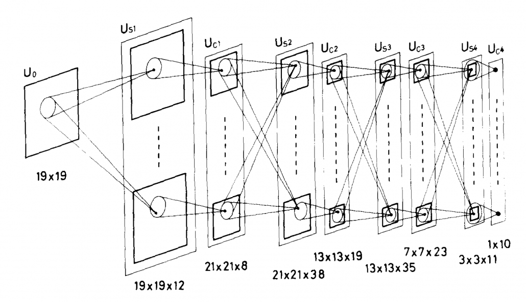
Source: Fukushima Kunihiko, “Neocognitron: A self-organizing neural network model for a mechanism of pattern recognition unaffected by shift in position,” (1980)

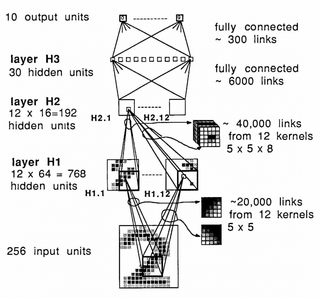
I am not going to write about the second AI boom in detail, but at least you should keep it in mind that convolutional neural network (CNN) is a keyword in this time. Neocognitron, an artificial model of how sight nerves perceive thing, was invented by Kunihiko Fukushima in 1980, and the model is said to be the origin on CNN. And Neocognitron got inspired by the Hubel and Wiesel’s research on sight nerves. In 1989, a group in AT & T Bell Laboratory led by Yann LeCun invented the first practical CNN to read handwritten digit.

Y. LeCun, “Backpropagation Applied to Handwritten Zip Code Recognition,” (1989)

Another turning point in this second AI boom was that back propagation algorithm was discovered, and the CNN by LeCun was also trained with back propagation. LeCun made a deep neural networks with some layers in 1998 for more practical uses.

But his research did not gain so much attention like today, because AI research entered its second winter at the beginning of the 1990s, and that was partly due to vanishing/exploding gradient problem of deep learning. People knew that neural networks had potentials of universal approximation, but when they tried to train naively stacked neural nets, the gradients, which you need for training neural networks, exponentially increased/decreased. Even though the CNN made by LeCun was the first successful case of “deep” neural nets which did not suffer from the vanishing/exploding gradient problem so much, deep learning research also stagnated in this time.

The ultimate goal of this article series is to understand LSTM at a more abstract/mathematical level because it is one of the practical RNNs, but the idea of LSTM (Long Short Term Memory) itself was already proposed in 1997 as an RNN algorithm to tackle vanishing gradient problem. (Exploding gradient problem is solved with a technique named gradient clipping, and this is easier than techniques for preventing vanishing gradient problems. I am also going to explain it in the next article.) After that some other techniques like introducing forget gate, peephole connections, were discovered, but basically it took some 20 years till LSTM got attentions like today. The reasons for that is lack of hardware and data sets, and that was also major reasons for the second AI winter.

Source: Sepp HochreiterJürgen, Schmidhuber, “Long Short-term Memory,” (1997)

In the 1990s, the mid of second AI winter, the Internet started prevailing for commercial uses. I think one of the iconic events in this time was the source codes WWW (World Wide Web) were announced in 1993. Some of you might still remember that you little by little became able to transmit more data online in this time. That means people came to get more and more access to various datasets in those days, which is indispensable for machine learning tasks.

After all, we could not get HAL 9000 by the end of 2001, but instead we got Xbox console.

3, Video game industry and GPU

Even though research on neural networks stagnated in the 1990s the same period witnessed an advance in the computation of massive parallel linear transformations, due to their need in fields such as image processing.

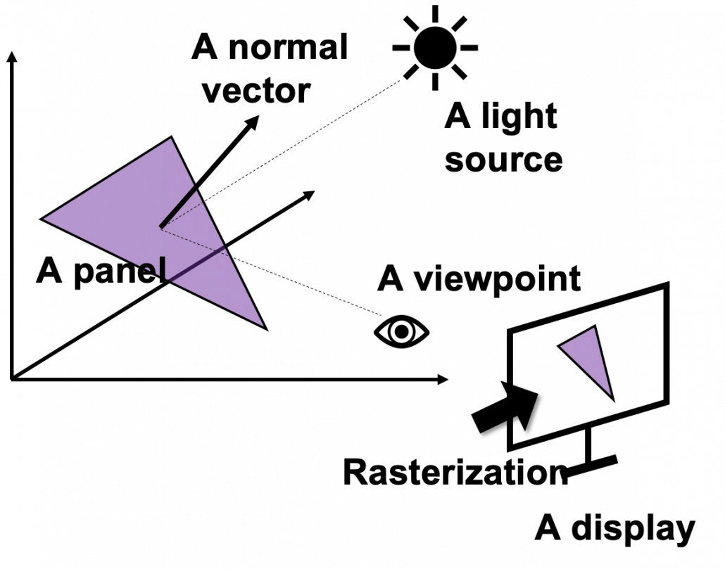
Computer graphics move or rotate in 3d spaces, and that is also linear transformations. When you think about a car moving in a city, it is convenient to place the car, buildings, and other objects on a fixed 3d space. But when you need to make computer graphics of scenes of the city from a view point inside the car, you put a moving origin point in the car and see the city. The spatial information of the city is calculated as vectors from the moving origin point. Of course this is also linear transformations. Of course I am not talking about a dot or simple figures moving in the 3d spaces. Computer graphics are composed of numerous plane panels, and each of them have at least three vertexes, and they move on 3d spaces. Depending on viewpoints, you need project the 3d graphics in 3d spaces on 2d spaces to display the graphics on devices. You need to calculate which part of the panel is projected to which pixel on the display, and that is called rasterization. Plus, in order to get photophotorealistic image, you need to think about how lights from light sources reflect on the panel and projected on the display. And you also have to put some textures on groups of panels. You might also need to change color spaces, which is also linear transformations.

My point is, in short, you really need to do numerous linear transformations in parallel in image processing.

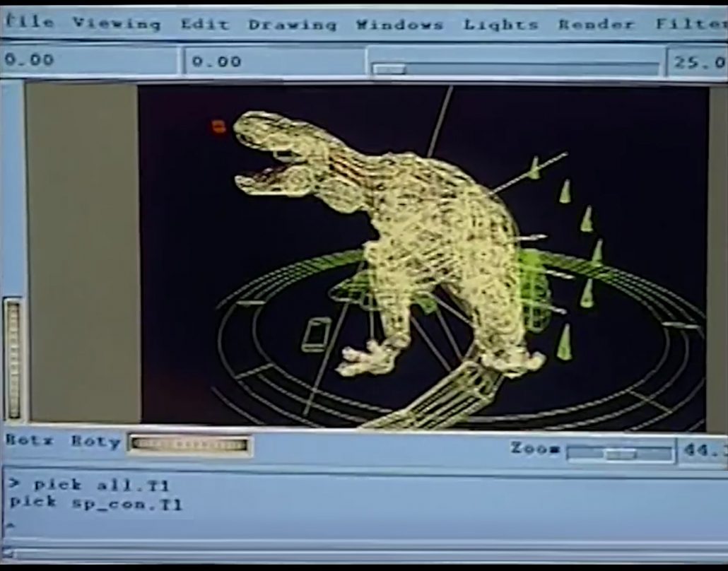
When it comes to the use of CGI in movies, two pioneer movies were released during this time: Jurassic Park in 1993, and Toy Story in 1995. It is famous that Pixar used to be one of the departments in ILM (Industrial Light and Magic), founded by George Lucas, and Steve Jobs bought the department. Even though the members in Pixar had not even made a long feature film in their lives, after trial and errors, they made the first CGI animated feature movie. On the other hand, in order to acquire funds for the production of Schindler’s List (1993), Steven Spielberg took on Jurassic Park (1993), consequently changing the history of CGI through this “side job.”

Source: http://renderstory.com/jurassic-park-23-years-later/

*I think you have realized that George Lucas is mentioned almost everywhere in this article. His influences on technologies are not only limited to image processing, but also sound measuring system, nonlinear editing system. Photoshop was also originally developed under his company. I need another article series for this topic, but maybe not in Data Science Blog.

Source: https://editorial.rottentomatoes.com/article/5-technical-breakthroughs-in-star-wars-that-changed-movies-forever/

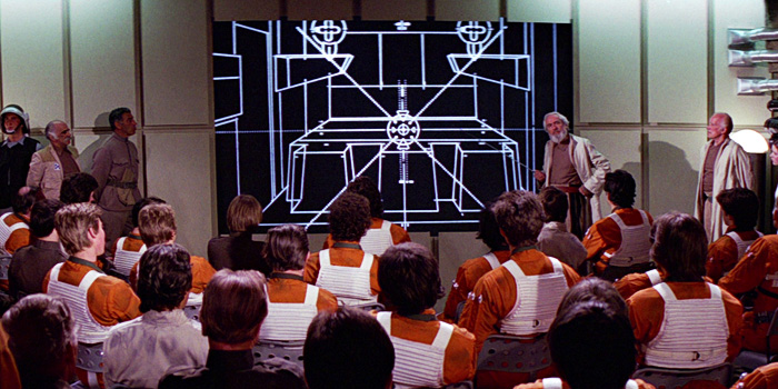
Considering that the first wire-frame computer graphics made and displayed by computers appeared in the scene of displaying the wire frame structure of Death Star in a war room, in Star Wars: A New Hope, the development of CGI was already astonishing at this time. But I think deep learning owe its development more to video game industry.

*I said that the Death Star scene is the first use of graphics made and DISPLAYED by computers, because I have to say one of the first graphics in movie MADE by computer dates back to the legendary title sequence of Vertigo(1958).

When it comes to 3D video games the processing unit has to constantly deal with real time commands from controllers. It is famous that GPU was originally specifically designed for plotting computer graphics. Video game market is the biggest in entertainment industry in general, and it is said that the quality of computer graphics have the strongest correlation with video games sales, therefore enhancing this quality is a priority for the video game console manufacturers.

One good example to see how much video games developed is comparing original Final Fantasy 7 and the remake one. The original one was released in 1997, the same year as when LSTM was invented. And recently the remake version of Final Fantasy 7 was finally released this year. The original one was also made with very big budget, and it was divided into three CD-ROMs. The original one was also very revolutionary given that the former ones of Final Fantasy franchise were all 2d video retro style video games. But still the computer graphics looks like polygons, and in almost all scenes the camera angle was fixed in the original one. On the other hand the remake one is very photorealistic and you can move the angle of the camera as you want while you play the video game.

There were also fierce battles by graphic processor manufacturers in computer video game market in the 1990s, but personally I think the release of Xbox console was a turning point in the development of GPU. To be concrete, Microsoft adopted a type of NV20 GPU for Xbox consoles, and that left some room of programmability for developers. The chief architect of NV20, which was released under the brand of GeForce3, said making major changes in the company’s graphic chips was very risky. But that decision opened up possibilities of uses of GPU beyond computer graphics.

Source: https://de.wikipedia.org/wiki/Nvidia-GeForce-3-Serie

I think that the idea of a programmable GPU provided other scientific fields with more visible benefits after CUDA was launched. And GPU gained its position not only in deep learning, but also many other fields including making super computers.

*When it comes to deep learning, even GPUs have strong rivals. TPU(Tensor Processing Unit) made by Google, is specialized for deep learning tasks, and have astonishing processing speed. And FPGA(Field Programmable Gate Array), which was originally invented customizable electronic circuit, proved to be efficient for reducing electricity consumption of deep learning tasks.

*I am not so sure about this GPU part. Processing unit, including GPU is another big topic, that is beyond my capacity to be honest. I would appreciate it if you could share your view and some references to confirm your opinion, on the comment section or via email.

*If you are interested you should see this video of game fans’ reactions to the announcement of Final Fantasy 7. This is the industry which grew behind the development of deep learning, and many fields where you need parallel computations owe themselves to the nerds who spent a lot of money for video games, including me.

*But ironically the engineers who invented the GPU said they did not play video games simply because they were busy. If you try to study the technologies behind video games, you would not have much time playing them. That is the reality.

We have seen that the in this second AI winter, Internet and GPU laid foundation of the next AI boom. But still the last piece of the puzzle is missing: let’s look at the breakthrough which solved the vanishing /exploding gradient problem of deep learning in the next section.

4, Pretraining of deep belief networks: “The Dawn of Deep Learning”

Some researchers say the invention of pretraining of deep belief network by Geoffrey Hinton was a breakthrough which put an end to the last AI winter. Deep belief networks are different type of networks from the neural networks we have discussed, but their architectures are similar to those of the neural networks. And it was also unknown how to train deep belief nets when they have several layers. Hinton discovered that training the networks layer by layer in advance can tackle vanishing gradient problems. And later it was discovered that you can do pretraining neural networks layer by layer with autoencoders.

*Deep belief network is beyond the scope of this article series. I have to talk about generative models, Boltzmann machine, and some other topics.

The pretraining techniques of neural networks is not mainstream anymore. But I think it is very meaningful to know that major deep learning techniques such as using ReLU activation functions, optimization with Adam, dropout, batch normalization, came up as more effective algorithms for deep learning after the advent of the pretraining techniques, and now we are in the third AI boom.

In the next next article we are finally going to work on LSTM. Specifically, I am going to offer a clearer guide to a well-made paper on LSTM, named “LSTM: A Search Space Odyssey.”

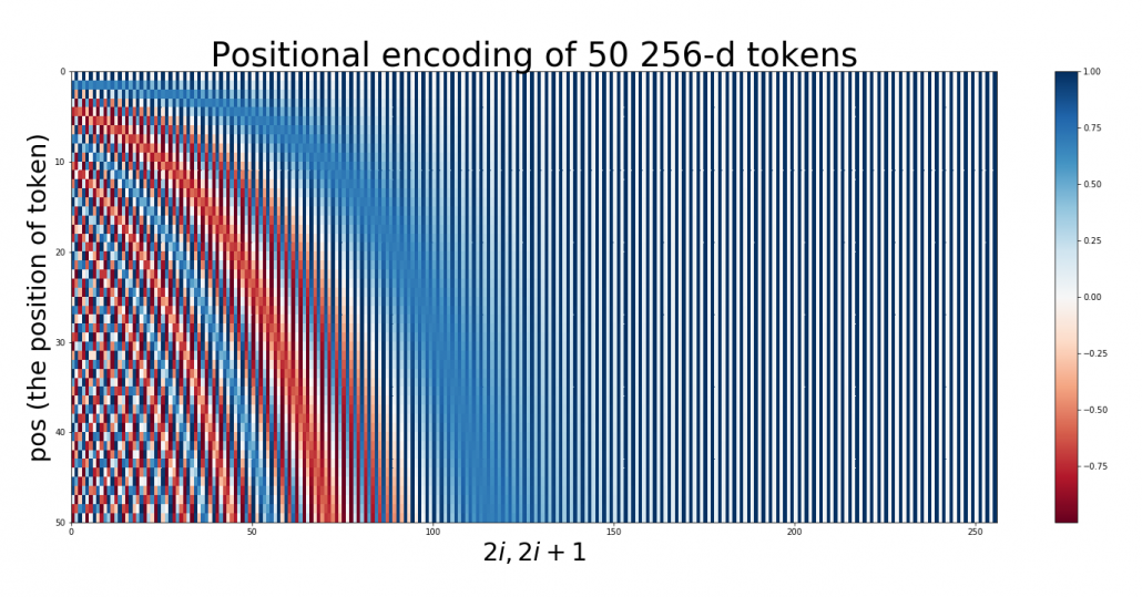
[References]

[1] Taniguchi Tadahiro, “An Illustrated Guide to Artificial Intelligence”, (2010), Kodansha pp. 3-11
谷口忠大著, 「イラストで学ぶ人工知能概論」, (2010), 講談社, pp. 3-11

[2] Francois Chollet, Deep Learning with Python,(2018), Manning , pp. 14-24

[3] Oketani Takayuki, “Machine Learning Professional Series: Deep Learning,” (2015), pp. 1-5, 151-156
岡谷貴之著, 「機械学習プロフェッショナルシリーズ深層学習」, (2015), pp. 1-5, 151-156

[4] Abigail See, Matthew Lamm, “Natural Language Processingwith Deep LearningCS224N/Ling284 Lecture 8:Machine Translation,Sequence-to-sequence and Attention,” (2020),
URL: http://web.stanford.edu/class/cs224n/slides/cs224n-2020-lecture08-nmt.pdf

[5]C. M. Bishop, “Pattern Recognition and Machine Learning,” (2006), Springer, pp. 192-196

[6] Daniel C. Dennett, “Cognitive Wheels: the Frame Problem of AI,” (1984), pp. 1-2

[7] Machiyama Tomohiro, “Understanding Cinemas of 1967-1979,” (2014), Yosensya, pp. 14-30
町山智浩著, 「＜映画の見方＞が分かる本」,(2014), 洋泉社, pp. 14-30

[8] Harada Tatsuya, “Machine Learning Professional Series: Image Recognition,” (2017), pp. 156-157
原田達也著, 「機械学習プロフェッショナルシリーズ画像認識」, (2017), pp. 156-157

[9] Suyama Atsushi, “Machine Learning Professional Series: Bayesian Deep Learning,” (2019)岡谷貴之須山敦志著, 「機械学習プロフェッショナルシリーズベイズ深層学習」, (2019)

[10] “Understandable LSTM ~ With the Current Trends,” Qiita, (2015)
「わかるLSTM ～最近の動向と共に」, Qiita, (2015)
URL: https://qiita.com/t_Signull/items/21b82be280b46f467d1b

[11] Hisa Ando, “WEB+DB PRESS plus series: Technologies Supporting Processors – The World Endlessly Pursuing Speed,” (2017), Gijutsu-hyoron-sya, pp 313-317
Hisa Ando, 「WEB+DB PRESS plusシリーズプロセッサを支える技術― 果てしなくスピードを追求する世界」, (2017), 技術評論社, pp. 313-317

[12] “Takahashi Yoshiki and Utamaru discuss George Lucas,” miyearnZZ Labo, (2016)
“高橋ヨシキと宇多丸　ジョージ・ルーカスを語る,” miyearnZZ Labo, (2016)
URL: https://miyearnzzlabo.com/archives/38865

[13] Katherine Bourzac, “Chip Hall of Fame: Nvidia NV20 The first configurable graphics processor opened the door to a machine-learning revolution,” IEEE SPECTRUM, (2018)
URL: https://spectrum.ieee.org/tech-history/silicon-revolution/chip-hall-of-fame-nvidia-nv20

Einführung in die Welt der Autoencoder

April 1, 2020/in Artificial Intelligence, Big Data, Data Mining, Data Science, Data Science Hack, Deep Learning, Main Category, Python, TensorFlow, Tutorial/by Hoang Tu Nguyen

An wen ist der Artikel gerichtet?

In diesem Artikel wollen wir uns näher mit dem neuronalen Netz namens Autoencoder beschäftigen und wollen einen Einblick in die Grundprinzipien bekommen, die wir dann mit einem vereinfachten Programmierbeispiel festigen. Kenntnisse in Python, Tensorflow und neuronalen Netzen sind dabei sehr hilfreich.

Funktionsweise des Autoencoders

Ein Autoencoder ist ein neuronales Netz, welches versucht die Eingangsinformationen zu komprimieren und mit den reduzierten Informationen im Ausgang wieder korrekt nachzubilden.

Die Komprimierung und die Rekonstruktion der Eingangsinformationen laufen im Autoencoder nacheinander ab, weshalb wir das neuronale Netz auch in zwei Abschnitten betrachten können.

Der Encoder

Der Encoder oder auch Kodierer hat die Aufgabe, die Dimensionen der Eingangsinformationen zu reduzieren, man spricht auch von Dimensionsreduktion. Durch diese Reduktion werden die Informationen komprimiert und es werden nur die wichtigsten bzw. der Durchschnitt der Informationen weitergeleitet. Diese Methode hat wie viele andere Arten der Komprimierung auch einen Verlust.

In einem neuronalen Netz wird dies durch versteckte Schichten realisiert. Durch die Reduzierung von Knotenpunkten in den kommenden versteckten Schichten werden die Kodierung bewerkstelligt.

Der Decoder

Nachdem das Eingangssignal kodiert ist, kommt der Decoder bzw. Dekodierer zum Einsatz. Er hat die Aufgabe mit den komprimierten Informationen die ursprünglichen Daten zu rekonstruieren. Durch Fehlerrückführung werden die Gewichte des Netzes angepasst.

Ein bisschen Mathematik

Das Hauptziel des Autoencoders ist, dass das Ausgangssignal dem Eingangssignal gleicht, was bedeutet, dass wir eine Loss Funktion haben, die L(x , y) entspricht.

$L(x, \hat{x})$

Unser Eingang soll mit x gekennzeichnet werden. Unsere versteckte Schicht soll h sein. Damit hat unser Encoder folgenden Zusammenhang h = f(x).

Die Rekonstruktion im Decoder kann mit r = g(h) beschrieben werden. Bei unserem einfachen Autoencoder handelt es sich um ein Feed-Forward Netz ohne rückkoppelten Anteil und wird durch Backpropagation oder zu deutsch Fehlerrückführung optimiert.

Formelzeichen	Bedeutung
$\mathbf{x}, \hat{\mathbf{x}}$	Eingangs-, Ausgangssignal
$\mathbf{W}, \hat{\mathbf{W}}$	Gewichte für En- und Decoder
$\mathbf{B}, \hat{\mathbf{B}}$	Bias für En- und Decoder
$\sigma, \hat{\sigma}$	Aktivierungsfunktion für En- und Decoder
$L$	Verlustfunktion

Unsere versteckte Schicht soll mit $\latex h$ gekennzeichnet werden. Damit besteht der Zusammenhang:

(1) $\begin{align*} \mathbf{h} &= f(\mathbf{x}) = \sigma(\mathbf{W}\mathbf{x} + \mathbf{B}) \\ \hat{\mathbf{x}} &= g(\mathbf{h}) = \hat{\sigma}(\hat{\mathbf{W}} \mathbf{h} + \hat{\mathbf{B}}) \\ \hat{\mathbf{x}} &= \hat{\sigma} \{ \hat{\mathbf{W}} \left[\sigma ( \mathbf{W}\mathbf{x} + \mathbf{B} )\right] + \hat{\mathbf{B}} \}\\ \end{align*}$

Für eine Optimierung mit der mittleren quadratischen Abweichung (MSE) könnte die Verlustfunktion wie folgt aussehen:

(2) $\begin{align*} L(\mathbf{x}, \hat{\mathbf{x}}) &= \mathbf{MSE}(\mathbf{x}, \hat{\mathbf{x}}) = \| \mathbf{x} - \hat{\mathbf{x}} \| ^2 &= \| \mathbf{x} - \hat{\sigma} \{ \hat{\mathbf{W}} \left[\sigma ( \mathbf{W}\mathbf{x} + \mathbf{B} )\right] + \hat{\mathbf{B}} \} \| ^2 \end{align*}$

Wir haben die Theorie und Mathematik eines Autoencoder in seiner Ursprungsform kennengelernt und wollen jetzt diese in einem (sehr) einfachen Beispiel anwenden, um zu schauen, ob der Autoencoder so funktioniert wie die Theorie es besagt.

Dazu nehmen wir einen One Hot (1 aus n) kodierten Datensatz, welcher die Zahlen von 0 bis 3 entspricht.

$\begin{align*} [1, 0, 0, 0] \ \widehat{=} \ 0 \\ [0, 1, 0, 0] \ \widehat{=} \ 1 \\ [0, 0, 1, 0] \ \widehat{=} \ 2 \\ [0, 0, 0, 1] \ \widehat{=} \ 3\\ \end{align*}$

Diesen Datensatz könnte wie folgt kodiert werden:

$\begin{align*} [1, 0, 0, 0] \ \widehat{=} \ 0 \ \widehat{=} \ [0, 0] \\ [0, 1, 0, 0] \ \widehat{=} \ 1 \ \widehat{=} \ [0, 1] \\ [0, 0, 1, 0] \ \widehat{=} \ 2 \ \widehat{=} \ [1, 0] \\ [0, 0, 0, 1] \ \widehat{=} \ 3 \ \widehat{=} \ [1, 1] \\ \end{align*}$

Damit hätten wir eine Dimensionsreduktion von vier auf zwei Merkmalen vorgenommen und genau diesen Vorgang wollen wir bei unserem Beispiel erreichen.

Programmierung eines einfachen Autoencoders

Typische Einsatzgebiete des Autoencoders sind neben der Dimensionsreduktion auch Bildaufarbeitung (z.B. Komprimierung, Entrauschen), Anomalie-Erkennung, Sequenz-to-Sequenz Analysen, etc.

Ausblick

Wir haben mit einem einfachen Beispiel die Funktionsweise des Autoencoders festigen können. Im nächsten Schritt wollen wir anhand realer Datensätze tiefer in gehen. Auch soll in kommenden Artikeln Variationen vom Autoencoder in verschiedenen Einsatzgebieten gezeigt werden.

Visual Question Answering with Keras – Part 1

July 29, 2019/in Artificial Intelligence, Data Science, Data Science Hack, Deep Learning, Insights, Machine Learning, Main Category, Predictive Analytics, TensorFlow/by Akshay Chavan

This is Part I of II of the Article Series Visual Question Answering with Keras

Making Computers Intelligent to answer from images

If we look closer in the history of Artificial Intelligence (AI), the Deep Learning has gained more popularity in the recent years and has achieved the human-level performance in the tasks such as Speech Recognition, Image Classification, Object Detection, Machine Translation and so on. However, as humans, not only we but also a five-year child can normally perform these tasks without much inconvenience. But the development of such systems with these capabilities has always considered an ambitious goal for the researchers as well as for developers.

In this series of blog posts, I will cover an introduction to something called VQA (Visual Question Answering), its available datasets, the Neural Network approach for VQA and its implementation in Keras and the applications of this challenging problem in real life.

Table of Contents:

1 Introduction

2 What is exactly Visual Question Answering?

3 Prerequisites

4 Datasets available for VQA

4.1 DAQUAR Dataset

4.2 CLEVR Dataset

4.3 FigureQA Dataset

4.4 VQA Dataset

5 Real-life applications of VQA

6 Conclusion

Introduction:

Let’s say you are given a below picture along with one question. Can you answer it?

I expect confidently you all say it is the Kitchen without much inconvenience which is also the right answer. Even a five-year child who just started to learn things might answer this question correctly.

Alright, but can you write a computer program for such type of task that takes image and question about the image as an input and gives us answer as output?

Before the development of the Deep Neural Network, this problem was considered as one of the difficult, inconceivable and challenging problem for the AI researcher’s community. However, due to the recent advancement of Deep Learning the systems are capable of answering these questions with the promising result if we have a required dataset.

Now I hope you have got at least some intuition of a problem that we are going to discuss in this series of blog posts. Let’s try to formalize the problem in the below section.

What is exactly Visual Question Answering?:

We can define, “Visual Question Answering(VQA) is a system that takes an image and natural language question about the image as an input and generates natural language answer as an output.”

VQA is a research area that requires an understanding of vision(Computer Vision) as well as text(NLP). The main beauty of VQA is that the reasoning part is performed in the context of the image. So if we have an image with the corresponding question then the system must able to understand the image well in order to generate an appropriate answer. For example, if the question is the number of persons then the system must able to detect faces of the persons. To answer the color of the horse the system need to detect the objects in the image. Many of these common problems such as face detection, object detection, binary object classification(yes or no), etc. have been solved in the field of Computer Vision with good results.

To summarize a good VQA system must be able to address the typical problems of CV as well as NLP.

To get a better feel of VQA you can try online VQA demo by CloudCV. You just go to this link and try uploading the picture you want and ask the related question to the picture, the system will generate the answer to it.

Prerequisites:

In the next post, I will walk you through the code for this problem using Keras. So I assume that you are familiar with:

Fundamental concepts of Machine Learning
Multi-Layered Perceptron
Convolutional Neural Network
Recurrent Neural Network (especially LSTM)
Gradient Descent and Backpropagation
Transfer Learning
Hyperparameter Optimization
Python and Keras syntax

Datasets available for VQA:

As you know problems related to the CV or NLP the availability of the dataset is the key to solve the problem. The complex problems like VQA, the dataset must cover all possibilities of questions answers in real-world scenarios. In this section, I will cover some of the datasets available for VQA.

4.1 DAQUAR Dataset:

The DAQUAR dataset is the first dataset for VQA that contains only indoor scenes. It shows the accuracy of 50.2% on the human baseline. It contains images from the NYU_Depth dataset.

Example of DAQUAR dataset

The main disadvantage of DAQUAR is the size of the dataset is very small to capture all possible indoor scenes.

4.2 CLEVR Dataset:

The CLEVR Dataset from Stanford contains the questions about the object of a different type, colors, shapes, sizes, and material.

It has

A training set of 70,000 images and 699,989 questions
A validation set of 15,000 images and 149,991 questions
A test set of 15,000 images and 14,988 questions

Image Source: https://cs.stanford.edu/people/jcjohns/clevr/?source=post_page

4.3 FigureQA Dataset:

FigureQA Dataset contains questions about the bar graphs, line plots, and pie charts. It has 1,327,368 questions for 100,000 images in the training set.

4.4 VQA Dataset:

As comapred to all datasets that we have seen so far VQA dataset is relatively larger. The VQA dataset contains open ended as well as multiple choice questions. VQA v2 dataset contains:

82,783 training images from COCO (common objects in context) dataset
40, 504 validation images and 81,434 validation images
443,757 question-answer pairs for training images
214,354 question-answer pairs for validation images.

As you might expect this dataset is very huge and contains 12.6 GB of training images only. I have used this dataset in the next post but a very small subset of it.

This dataset also contains abstract cartoon images. Each image has 3 questions and each question has 10 multiple choice answers.

Real-life applications of VQA:

There are many applications of VQA. One of the famous applications is to help visually impaired people and blind peoples. In 2016, Microsoft has released the “Seeing AI” app for visually impaired people to describe the surrounding environment around them. You can watch this video for the prototype of the Seeing AI app.

Another application could be on social media or e-commerce sites. VQA can be also used for educational purposes.

Conclusion:

I hope this explanation will give you a good idea of Visual Question Answering. In the next blog post, I will walk you through the code in Keras.

If you like my explanations, do provide some feedback, comments, etc. and stay tuned for the next post.

Understanding Dropout and implementing it on MNIST dataset

May 20, 2019/in Data Science Hack, Python, TensorFlow, Tutorial/by Sarthak Babbar

Over-fitting is a major problem in deep learning and a plethora of techniques have been introduced to prevent it. One of the most effective one is called “dropout”. Let’s use the analogy of a person going to gym for understanding this. Let’s say the person going to gym mostly uses his dominant arm, say his right arm to pick up weights. After some time, he notices that his dominant arm is developing a large muscle, but not the other arm. So, what can he do? Obviously, he needs to involve both his arms while training. Sometimes he should stop using his right arm, and use the left arm to lift weights and vice versa.

Something like this happens commonly in neural networks. Sometime one part of the network has very large weights and ends up dominating the training. While other part of the network remains weak and does not really play a role in the training. So, what dropout does to solve this problem, is it randomly shuts off some nodes and stop the gradients flowing through it. So, our forward and back propagation happen without those nodes. In that case the rest of the nodes need to pick up the slack and be more active in the training. We define a probability of the nodes getting dropped. For example, P=0.5 means there is a 50% chance a node will be dropped.

Figure 1 demonstrates the dropout technique, taken from the original research paper.

Our network can never rely on any given node because it can be squashed at any given time. Hence the network is forced to learn redundant representation for everything to make sure at least some of the information remains. Redundant representation leads our network to be more robust. It also acts as ensemble of many networks, since at every epoch random nodes are dropped, each time our network will be different. Ensemble of different networks perform better than a single network since they capture more randomness. Please note, only non-output nodes are dropped.

Let’s, look at the python code to implement dropout in a neural network:

100

101

102

103

104

105

106

107

108

109

110

from tensorflow.examples.tutorials.mnist import input_data

mnist = input_data.read_data_sets(".", one_hot=True, reshape=False)

import tensorflow as tf

# Parameters

learning_rate = 0.00001

epochs = 10

batch_size = 128

# Number of samples to calculate validation and accuracy

test_valid_size = 256

# Network Parameters

n_classes = 10 # MNIST total classes (0-9 digits)

dropout = 0.75 # Dropout, probability to keep units

# layers weight & bias

weights = {

'wc1': tf.Variable(tf.random_normal([5, 5, 1, 32])),

'wc2': tf.Variable(tf.random_normal([5, 5, 32, 64])),

'wd1': tf.Variable(tf.random_normal([7*7*64, 1024])),

'out': tf.Variable(tf.random_normal([1024, n_classes]))}

biases = {

'bc1': tf.Variable(tf.random_normal([32])),

'bc2': tf.Variable(tf.random_normal([64])),

'bd1': tf.Variable(tf.random_normal([1024])),

'out': tf.Variable(tf.random_normal([n_classes]))}

#function that implements Convolution layer

def conv2d(x, W, b, strides=1):

x = tf.nn.conv2d(x, W, strides=[1, strides, strides, 1], padding='SAME')

x = tf.nn.bias_add(x, b)

return tf.nn.relu(x)

#defining a function to implement maxpool layers

def maxpool2d(x, k=2):

return tf.nn.max_pool(x, ksize=[1, k, k, 1], strides=[1, k, k, 1], padding='SAME')

#Function that defines all the convolution layers.

def conv_net(x, weights, biases, dropout):

# Layer 1 - 28*28*1 to 14*14*32

conv1 = conv2d(x, weights['wc1'], biases['bc1'])

conv1 = maxpool2d(conv1, k=2)

# Layer 2 - 14*14*32 to 7*7*64

conv2 = conv2d(conv1, weights['wc2'], biases['bc2'])

conv2 = maxpool2d(conv2, k=2)

# Fully connected layer - 7*7*64 to 1024

fc1 = tf.reshape(conv2, [-1, weights['wd1'].get_shape().as_list()[0]])

fc1 = tf.add(tf.matmul(fc1, weights['wd1']), biases['bd1'])

fc1 = tf.nn.relu(fc1)

fc1 = tf.nn.dropout(fc1, dropout) # Implementing the dropout layer

# Output Layer - class prediction - 1024 to 10

out = tf.add(tf.matmul(fc1, weights['out']), biases['out'])

return out

# tf Graph input

x = tf.placeholder(tf.float32, [None, 28, 28, 1])

y = tf.placeholder(tf.float32, [None, n_classes])

keep_prob = tf.placeholder(tf.float32) # Keep probability for dropout layers

# Model

logits = conv_net(x, weights, biases, keep_prob)

# Define loss and optimizer

cost = tf.reduce_mean(tf.nn.softmax_cross_entropy_with_logits(logits=logits, labels=y))

optimizer = tf.train.GradientDescentOptimizer(learning_rate=learning_rate).minimize(cost)

# Accuracy

correct_pred = tf.equal(tf.argmax(logits, 1), tf.argmax(y, 1))

accuracy = tf.reduce_mean(tf.cast(correct_pred, tf.float32))

# Initializing the variables

init = tf.global_variables_initializer()

# Launch the graph

with tf.Session() as sess:

sess.run(init)

for epoch in range(epochs):

for batch in range(mnist.train.num_examples//batch_size):

batch_x, batch_y = mnist.train.next_batch(batch_size)

sess.run(optimizer, feed_dict={x: batch_x, y: batch_y, keep_prob: dropout})

# Calculate batch loss and accuracy

loss = sess.run(cost, feed_dict={x: batch_x, y: batch_y, keep_prob: 1.})

valid_acc = sess.run(accuracy, feed_dict={

x: mnist.validation.images[:test_valid_size],

y: mnist.validation.labels[:test_valid_size],

keep_prob: 1.}) #we want to keep all nodes while training so keep prob is 1.

print('Epoch {:>2}, Batch {:>3} - Loss: {:>10.4f} Validation Accuracy: {:.6f}'.format(

epoch + 1,

batch + 1,

loss,

valid_acc))

# Calculate Test Accuracy

test_acc = sess.run(accuracy, feed_dict={

x: mnist.test.images[:test_valid_size],

y: mnist.test.labels[:test_valid_size],

keep_prob: 1.})

print('Testing Accuracy: {}'.format(test_acc))

How to make a toy English-German translator with multi-head attention heat maps: the overall architecture of Transformer

1 The datasets

2 The whole architecture

3 The encoder

4, The decoder

5 Masking tokens in practice

6 Decoding process

Positional encoding, residual connections, padding masks: covering the rest of Transformer components

1 Wrapping points up so far

2 Why Transformer?

3 Positional encoding

5 Residual connections

6 Masked multi-head attention

Appendix

On the difficulty of language: prerequisites for NLP with deep learning

1 Preface

2 Tokens and word embedding

3 Language model

Appendix

[References]

A brief history of neural nets: everything you should know before learning LSTM

1, First AI boom

2, Second AI boom/winter

3, Video game industry and GPU

4, Pretraining of deep belief networks: “The Dawn of Deep Learning”

Einführung in die Welt der Autoencoder

An wen ist der Artikel gerichtet?

Funktionsweise des Autoencoders

Der Encoder

Der Decoder

Ein bisschen Mathematik

Programmierung eines einfachen Autoencoders

Ausblick

Visual Question Answering with Keras – Part 1

Understanding Dropout and implementing it on MNIST dataset

Interesting links

Pages

Categories

Archive