Predictive maintenance in Semiconductor Industry: Part 1
The process in the semiconductor industry is highly complicated and is normally under consistent observation via the monitoring of the signals coming from several sensors. Thus, it is important for the organization to detect the fault in the sensor as quickly as possible. There are existing traditional statistical based techniques however modern semiconductor industries have the ability to produce more data which is beyond the capability of the traditional process.
For this article, we will be using SECOM dataset which is available here. A lot of work has already done on this dataset by different authors and there are also some articles available online. In this article, we will focus on problem definition, data understanding, and data cleaning.
This article is only the first of three parts, in this article we will discuss the business problem in hand and clean the dataset. In second part we will do feature engineering and in the last article we will build some models and evaluate them.
Problem definition
This data which is collected by these sensors not only contains relevant information but also a lot of noise. The dataset contains readings from 590. Among the 1567 examples, there are only 104 fail cases which means that out target variable is imbalanced. We will look at the distribution of the dataset when we look at the python code.
NOTE: For a detailed description regarding this cases study I highly recommend to read the following research papers:
- Kerdprasop, K., & Kerdprasop, N. A Data Mining Approach to Automate Fault Detection Model Development in the Semiconductor Manufacturing Process.
- Munirathinam, S., & Ramadoss, B. Predictive Models for Equipment Fault Detection in the Semiconductor Manufacturing Process.
Data Understanding and Preparation
Let’s start exploring the dataset now. The first step as always is to import the required libraries.
|
1 2 |
import pandas as pd import numpy as np |
There are several ways to import the dataset, you can always download and then import from your working directory. However, I will directly import using the link. There are two datasets: one contains the readings from the sensors and the other one contains our target variable and a timestamp.
|
1 2 3 4 5 6 7 8 |
# Load dataset url = "https://archive.ics.uci.edu/ml/machine-learning-databases/secom/secom.data" names = ["feature" + str(x) for x in range(1, 591)] secom_var = pd.read_csv(url, sep=" ", names=names, na_values = "NaN") url_l = "https://archive.ics.uci.edu/ml/machine-learning-databases/secom/secom_labels.data" secom_labels = pd.read_csv(url_l,sep=" ",names = ["classification","date"],parse_dates = ["date"],na_values = "NaN") |
The first step before doing the analysis would be to merge the dataset and we will us pandas library to merge the datasets in just one line of code.
|
1 2 3 |
#Data cleaning #1. Combined the two datasets secom_merged = pd.merge(secom_var, secom_labels,left_index=True,right_index=True) |
Now let’s check out the distribution of the target variable
|
1 |
secom_merged.target.value_counts().plot(kind = 'bar') |
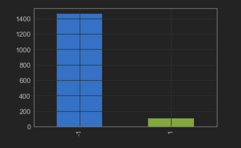
From Figure 1 it can be observed that the target variable is imbalanced and it is highly recommended to deal with this problem before the model building phase to avoid bias model. Xgboost is one of the models which can deal with imbalance classes but one needs to spend a lot of time to tune the hyper-parameters to achieve the best from the model.
The dataset in hand contains a lot of null values and the next step would be to analyse these null values and remove the columns having null values more than a certain percentage. This percentage is calculated based on 95th quantile of null values.
|
1 2 3 4 5 |
#2. Analyzing nulls secom_rmNa.isnull().sum().sum() secom_nulls = secom_rmNa.isnull().sum()/len(secom_rmNa) secom_nulls.describe() secom_nulls.hist() |
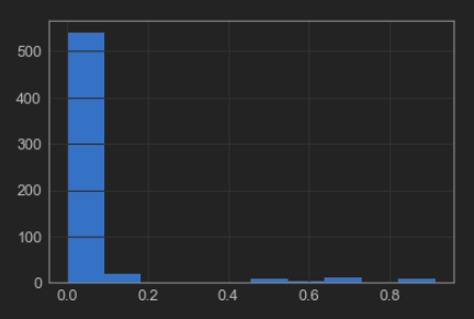
Now we calculate the 95th percentile of the null values.
|
1 2 |
x = secom_nulls.quantile(0.95) secom_rmNa = secom_merged[secom_merged.columns[secom_nulls < x]] |
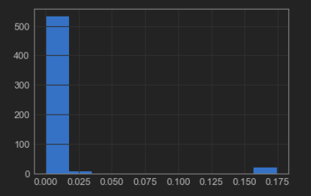
From figure 3 its visible that there are still missing values in the dataset and can be dealt by using many imputation methods. The most common method is to impute these values by mean, median or mode. There also exist few sophisticated techniques like K-nearest neighbour and interpolation. We will be applying interpolation technique to our dataset.
|
1 |
secom_complete = secom_rmNa.interpolate() |
To prepare our dataset for analysis we should remove some more unwanted columns like columns with near zero variance. For this we can calulate number of unique values in each column and if there is only one unique value we can delete the column as it holds no information.
|
1 2 3 4 5 |
df = secom_complete.loc[:,secom_complete.apply(pd.Series.nunique) != 1] ## Let's check the shape of the df df.shape (1567, 444) |
We have applied few data cleaning techniques and reduced the features from 590 to 444. However, In the next article we will apply some feature engineering techniques and adress problems like the curse of dimensionality and will also try to balance the target variable.
Bleiben Sie dran!!








Hi Aakash,
very interesting writing! I couldn’t find part 2 of your analysis. Did you published it?
Best
Nicolas