Variational Autoencoders

After Deep Autoregressive Models and Deep Generative Modelling, we will continue our discussion with Variational AutoEncoders (VAEs) after covering up DGM basics and AGMs. Variational autoencoders (VAEs) are a deep learning method to produce synthetic data (images, texts) by learning the latent representations of the training data. AGMs are sequential models and generate data based on previous data points by defining tractable conditionals. On the other hand, VAEs are using latent variable models to infer hidden structure in the underlying data by using the following intractable distribution function:

(1) $\begin{equation*} p_\theta(x) = \int p_\theta(x|z)p_\theta(z) dz. \end{equation*}$

The generative process using the above equation can be expressed in the form of a directed graph as shown in Figure ?? (the decoder part), where latent variable $z\sim p_\theta(z)$ produces meaningful information of $x \sim p_\theta(x|z)$ .

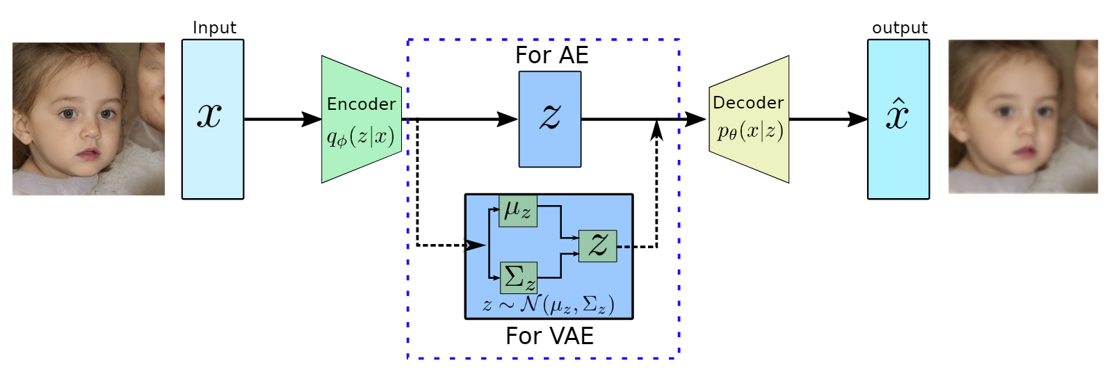
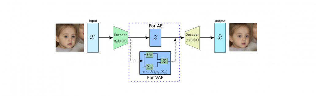
Figure 1: Architectures AE and VAE based on the bottleneck architecture. The decoder part work as
a generative model during inference.

Autoencoders

Autoencoders (AEs) are the key part of VAEs and are an unsupervised representation learning technique and consist of two main parts, the encoder and the decoder (see Figure ??). The encoders are deep neural networks (mostly convolutional neural networks with imaging data) to learn a lower-dimensional feature representation from training data. The learned latent feature representation $z$ usually has a much lower dimension than input $x$ and has the most dominant features of $x$ . The encoders are learning features by performing the convolution at different levels and compression is happening via max-pooling.

On the other hand, the decoders, which are also a deep convolutional neural network are reversing the encoder’s operation. They try to reconstruct the original data $x$ from the latent representation $z$ using the up-sampling convolutions. The decoders are pretty similar to VAEs generative models as shown in Figure 1, where synthetic images will be generated using the latent variable $z$ .

During the training of autoencoders, we would like to utilize the unlabeled data and try to minimize the following quadratic loss function:

(2) $\begin{equation*} \mathcal{L}(\theta, \phi) = ||x-\hat{x}||^2, \end{equation*}$

The above equation tries to minimize the distance between the original input and reconstructed image as shown in Figure 1.

Variational autoencoders

VAEs are motivated by the decoder part of AEs which can generate the data from latent representation and they are a probabilistic version of AEs which allows us to generate synthetic data with different attributes. VAE can be seen as the decoder part of AE, which learns the set parameters $\theta$ to approximate the conditional $p_\theta(x|z)$ to generate images based on a sample from a true prior, $z\sim p_\theta(z)$ . The true prior $p_\theta(z)$ are generally of Gaussian distribution.

Network Architecture

VAE has a quite similar architecture to AE except for the bottleneck part as shown in Figure 2. in AES, the encoder converts high dimensional input data to low dimensional latent representation in a vector form. On the other hand, VAE’s encoder learns the mean vector and standard deviation diagonal matrix such that $z\sim \matcal{N}(\mu_z, \Sigma_x)$ as it will be performing probabilistic generation of data. Therefore the encoder and decoder should be probabilistic.

Training

Similar to AGMs training, we would like to maximize the likelihood of the training data. The likelihood of the data for VAEs are mentioned in Equation 1 and the first term $p_\theta(x|z)$ will be approximated by neural network and the second term $p(x)$ prior distribution, which is a Gaussian function, therefore, both of them are tractable. However, the integration won’t be tractable because of the high dimensionality of data.

To solve this problem of intractability, the encoder part of AE was utilized to learn the set of parameters $\phi$ to approximate the conditional $q_\phi (z|x)$ . Furthermore, the conditional $q_\phi (z|x)$ will approximate the posterior $p_\theta (z|x)$ , which is intractable. This additional encoder part will help to derive a lower bound on the data likelihood that will make the likelihood function tractable. In the following we will derive the lower bound of the likelihood function:

(3) $\begin{equation*} \begin{flalign} \begin{aligned} log \: p_\theta (x) = & \mathbf{E}_{z\sim q_\phi(z|x)} \Bigg[log \: \frac{p_\theta (x|z) p_\theta (z)}{p_\theta (z|x)} \: \frac{q_\phi(z|x)}{q_\phi(z|x)}\Bigg] \\ = & \mathbf{E}_{z\sim q_\phi(z|x)} \Bigg[log \: p_\theta (x|z)\Bigg] - \mathbf{E}_{z\sim q_\phi(z|x)} \Bigg[log \: \frac{q_\phi (z|x)} {p_\theta (z)}\Bigg] + \mathbf{E}_{z\sim q_\phi(z|x)} \Bigg[log \: \frac{q_\phi (z|x)}{p_\theta (z|x)}\Bigg] \\ = & \mathbf{E}_{z\sim q_\phi(z|x)} \Big[log \: p_\theta (x|z)\Big] - \mathbf{D}_{KL}(q_\phi (z|x), p_\theta (z)) + \mathbf{D}_{KL}(q_\phi (z|x), p_\theta (z|x)). \end{aligned} \end{flalign} \end{equation*}$

In the above equation, the first line computes the likelihood using the logarithmic of $p_\theta (x)$ and then it is expanded using Bayes theorem with additional constant $q_\phi(z|x)$ multiplication. In the next line, it is expanded using the logarithmic rule and then rearranged. Furthermore, the last two terms in the second line are the definition of KL divergence and the third line is expressed in the same.

In the last line, the first term is representing the reconstruction loss and it will be approximated by the decoder network. This term can be estimated by the reparametrization trick \cite{}. The second term is KL divergence between prior distribution $p_\theta(z)$ and the encoder function $q_\phi (z|x)$ , both of these functions are following the Gaussian distribution and has the closed-form solution and are tractable. The last term is intractable due to $p_\theta (z|x)$ . However, KL divergence computes the distance between two probability densities and it is always positive. By using this property, the above equation can be approximated as:

(4) $\begin{equation*} log \: p_\theta (x)\geq \mathcal{L}(x, \phi, \theta) , \: \text{where} \: \mathcal{L}(x, \phi, \theta) = \mathbf{E}_{z\sim q_\phi(z|x)} \Big[log \: p_\theta (x|z)\Big] - \mathbf{D}_{KL}(q_\phi (z|x), p_\theta (z)). \end{equation*}$

In the above equation, the term $\mathcal{L}(x, \phi, \theta)$ is presenting the tractable lower bound for the optimization and is also termed as ELBO (Evidence Lower Bound Optimization). During the training process, we maximize ELBO using the following equation:

(5) $\begin{equation*} \operatorname*{argmax}_{\phi, \theta} \sum_{x\in X} \mathcal{L}(x, \phi, \theta). \end{equation*}$

Furthermore, the reconstruction loss term can be written using Equation 2 as the decoder output is assumed to be following Gaussian distribution. Therefore, this term can be easily transformed to mean squared error (MSE).

During the implementation, the architecture part is straightforward and can be found here. The user has to define the size of latent space, which will be vital in the reconstruction process. Furthermore, the loss function can be minimized using ADAM optimizer with a fixed batch size and a fixed number of epochs.

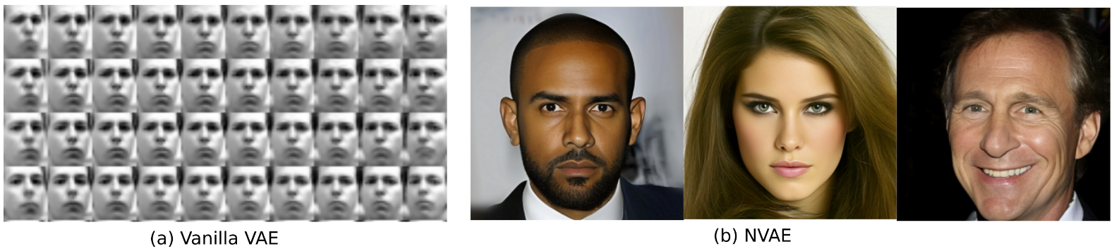
Figure 2: The results obtained from vanilla VAE (left) and a recent VAE-based generative
model NVAE (right)

In the above, we are showing the quality improvement since VAE was introduced by Kingma and
Welling [KW14]. NVAE is a relatively new method using a deep hierarchical VAE [VK21].

Summary

In this blog, we discussed variational autoencoders along with the basics of autoencoders. We covered
the main difference between AEs and VAEs along with the derivation of lower bound in VAEs. We
have shown using two different VAE based methods that VAE is still active research because in general,
it produces a blurry outcome.

References

[KW14] Diederik P Kingma and Max Welling. Auto-encoding variational bayes, 2014.
[VK21] Arash Vahdat and Jan Kautz. Nvae: A deep hierarchical variational autoencoder, 2021.

About Author

Sunil Yadav

Sunil Yadav is an experienced researcher with a keen focus on applying academic research to solve real-world problems. He believes a research paper has more value if it can be used for the welfare of society in general and the wellness of people in particular. He finished his PhD in mathematics and computer science and has a focus on computer vision, 3D data modelling, and medical imaging. His research interests revolve around understanding the visual data and producing meaningful output using the different areas of mathematics, including Deep learning, Machine learning, and computer vision.

See author's posts