Machine Learning Archives

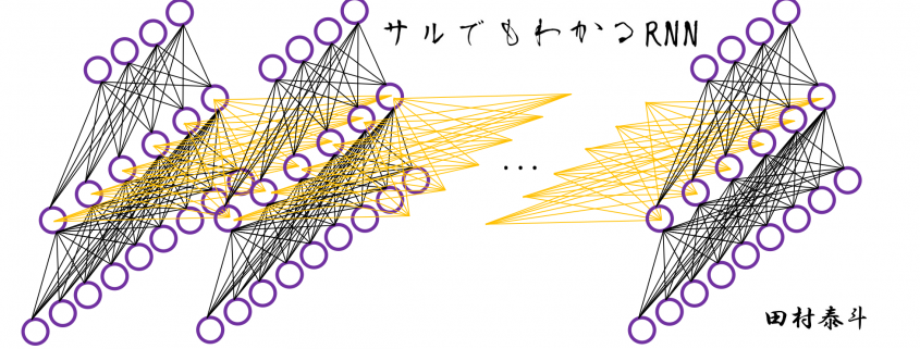
Simple RNN: the first foothold for understanding LSTM

June 17, 2020/in Artificial Intelligence, Data Science, Deep Learning, Machine Learning, Main Category, Mathematics/by Yasuto Tamura

*In this article “Densely Connected Layers” is written as “DCL,” and “Convolutional Neural Network” as “CNN.”

In the last article, I mentioned “When it comes to the structure of RNN, many study materials try to avoid showing that RNNs are also connections of neurons, as well as DCL or CNN.” Even if you manage to understand DCL and CNN, you can be suddenly left behind once you try to understand RNN because it looks like a different field. In the second section of this article, I am going to provide a some helps for more abstract understandings of DCL/CNN , which you need when you read most other study materials.

My explanation on this simple RNN is based on a chapter in a textbook published by Massachusetts Institute of Technology, which is also recommended in some deep learning courses of Stanford University.

First of all, you should keep it in mind that simple RNN are not useful in many cases, mainly because of vanishing/exploding gradient problem, which I am going to explain in the next article. LSTM is one major type of RNN used for tackling those problems. But without clear understanding forward/back propagation of RNN, I think many people would get stuck when they try to understand how LSTM works, especially during its back propagation stage. If you have tried climbing the mountain of understanding LSTM, but found yourself having to retreat back to the foot, I suggest that you read through this article on simple RNNs. It should help you to gain a solid foothold, and you would be ready for trying to climb the mountain again.

*This article is the second article of “A gentle introduction to the tiresome part of understanding RNN.”

1, A brief review on back propagation of DCL.

Simple RNNs are straightforward applications of DCL, but if you do not even have any ideas on DCL forward/back propagation, you will not be able to understand this article. If you more or less understand how back propagation of DCL works, you can skip this first section.

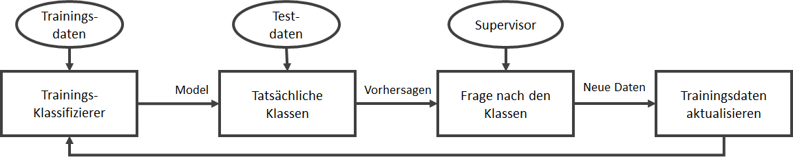
Deep learning is a part of machine learning. And most importantly, whether it is classical machine learning or deep learning, adjusting parameters is what machine learning is all about. Parameters mean elements of functions except for variants. For example when you get a very simple function $f(x)=a + bx + cx^2 + dx^3$ , then $x$ is a variant, and $a, b, c, d$ are parameters. In case of classical machine learning algorithms, the number of those parameters are very limited because they were originally designed manually. Such functions for classical machine learning is useful for features found by humans, after trial and errors(feature engineering is a field of finding such effective features, manually). You adjust those parameters based on how different the outputs(estimated outcome of classification/regression) are from supervising vectors(the data prepared to show ideal answers).

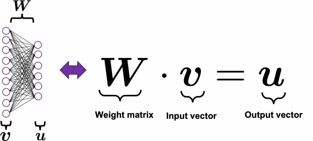
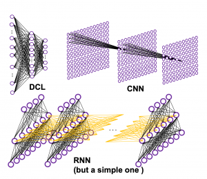
In the last article I said neural networks are just mappings, whose inputs are vectors, matrices, or sequence data. In case of DCLs, inputs are vectors. Then what’s the number of parameters ? The answer depends on the the number of neurons and layers. In the example of DCL at the right side, the number of the connections of the neurons is the number of parameters(Would you like to try to count them? At least I would say “No.”). Unlike classical machine learning you no longer need to do feature engineering, but instead you need to design networks effective for each task and adjust a lot of parameters.

*I think the hype of AI comes from the fact that neural networks find features automatically. But the reality is difficulty of feature engineering was just replaced by difficulty of designing proper neural networks.

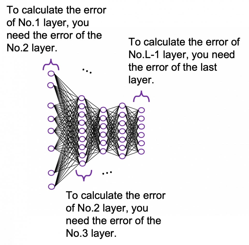
It is easy to imagine that you need an efficient way to adjust those parameters, and the method is called back propagation (or just backprop). As long as it is about DCL backprop, you can find a lot of well-made study materials on that, so I am not going to cover that topic precisely in this article series. Simply putting, during back propagation, in order to adjust parameters of a layer you need errors in the next layer. And in order calculate the errors of the next layer, you need errors in the next next layer.

*You should not think too much about what the “errors” exactly mean. Such “errors” are defined in this context, and you will see why you need them if you actually write down all the mathematical equations behind backprops of DCL.

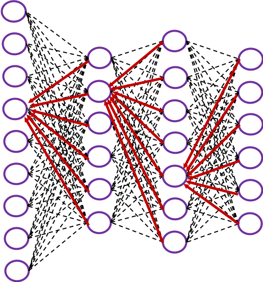
The red arrows in the figure shows how errors of all the neurons in a layer propagate backward to a neuron in last layer. The figure shows only some sets of such errors propagating backward, but in practice you have to think about all the combinations of such red arrows in the whole back propagation(this link would give you some ideas on how DCLs work).

These points are minimum prerequisites for continuing reading this RNN this article. But if you are planning to understand RNN forward/back propagation at an abstract/mathematical level that you can read academic papers, I highly recommend you to actually write down all the equations of DCL backprop. And if possible you should try to implement backprop of three-layer DCL.

2, Forward propagation of simple RNN

*For better understandings of the second and third section, I recommend you to download an animated PowerPoint slide which I prepared. It should help you understand simple RNNs.

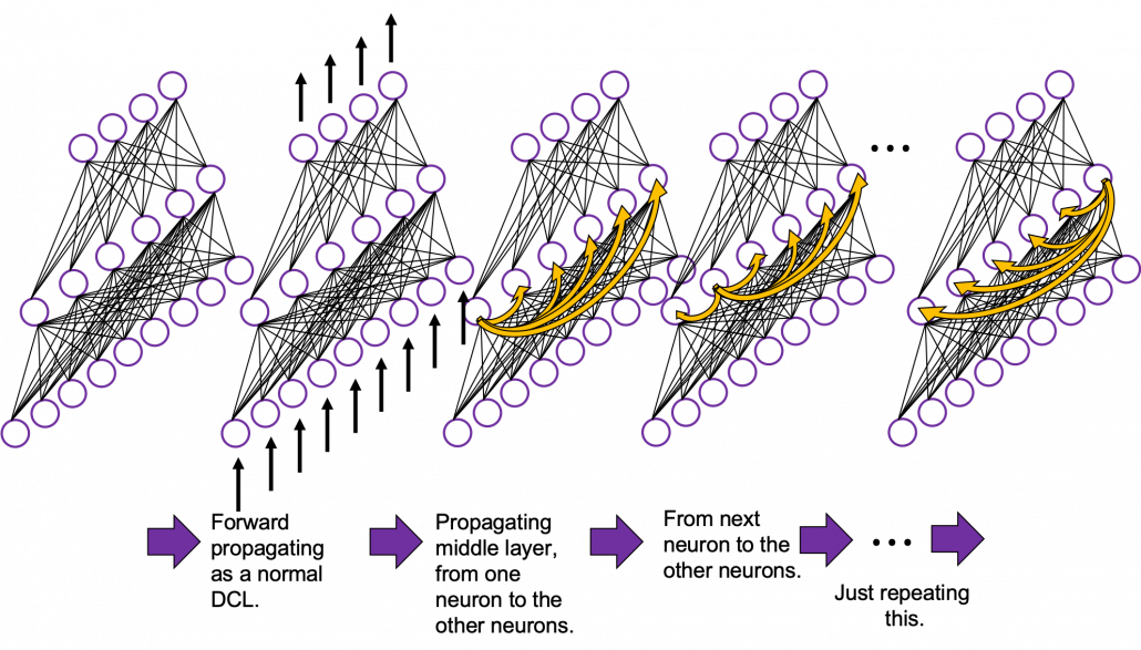
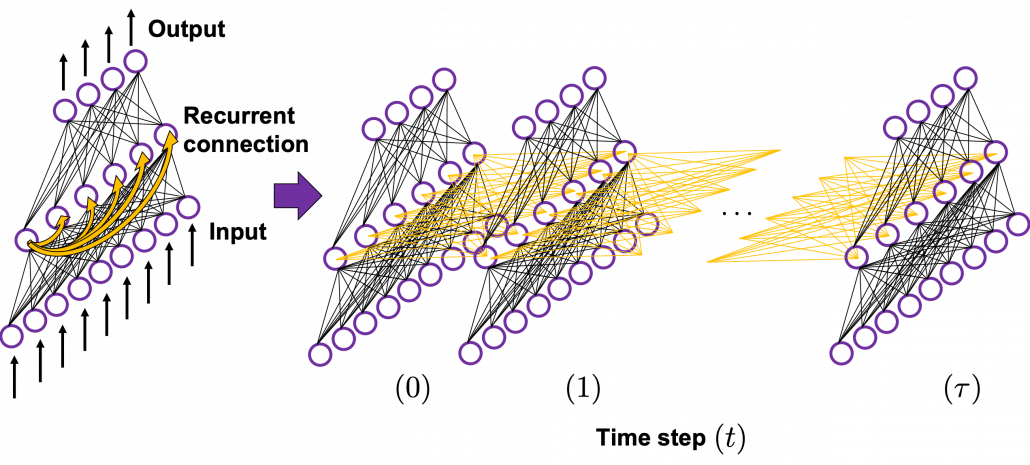
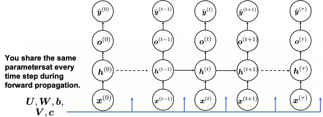
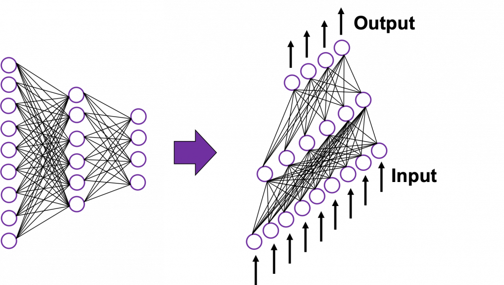In fact the simple RNN which we are going to look at in this article has only three layers. From now on imagine that inputs of RNN come from the bottom and outputs go up. But RNNs have to keep information of earlier times steps during upcoming several time steps because as I mentioned in the last article RNNs are used for sequence data, the order of whose elements is important. In order to do that, information of the neurons in the middle layer of RNN propagate forward to the middle layer itself. Therefore in one time step of forward propagation of RNN, the input at the time step propagates forward as normal DCL, and the RNN gives out an output at the time step. And information of one neuron in the middle layer propagate forward to the other neurons like yellow arrows in the figure. And the information in the next neuron propagate forward to the other neurons, and this process is repeated. This is called recurrent connections of RNN.

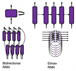
*To be exact we are just looking at a type of recurrent connections. For example Elman RNNs have simpler recurrent connections. And recurrent connections of LSTM are more complicated.

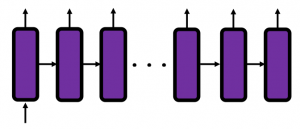
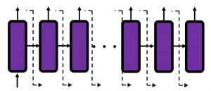
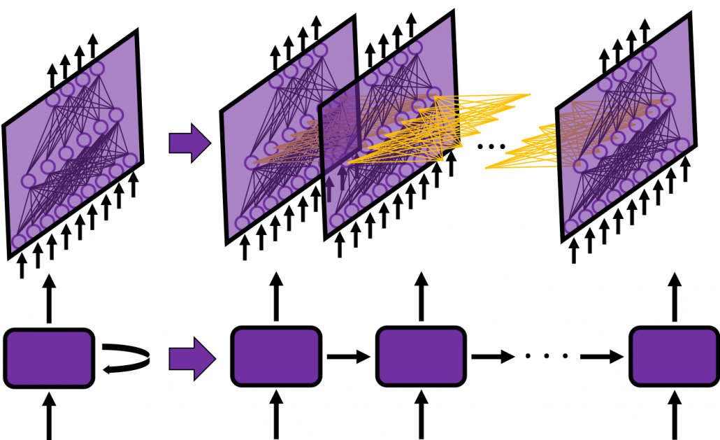
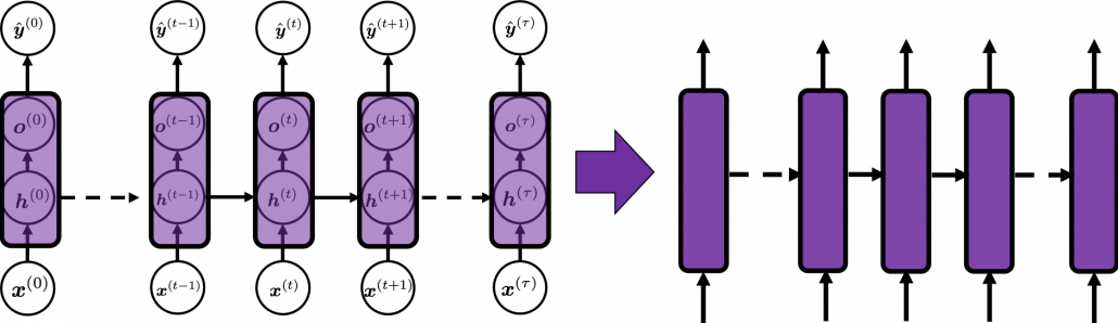
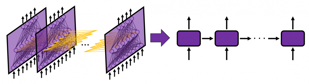
Whether it is a simple one or not, basically RNN repeats this process of getting an input at every time step, giving out an output, and making recurrent connections to the RNN itself. But you need to keep the values of activated neurons at every time step, so virtually you need to consider the same RNNs duplicated for several time steps like the figure below. This is the idea of unfolding RNN. Depending on contexts, the whole unfolded DCLs with recurrent connections is also called an RNN.

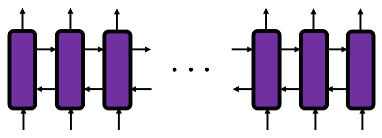
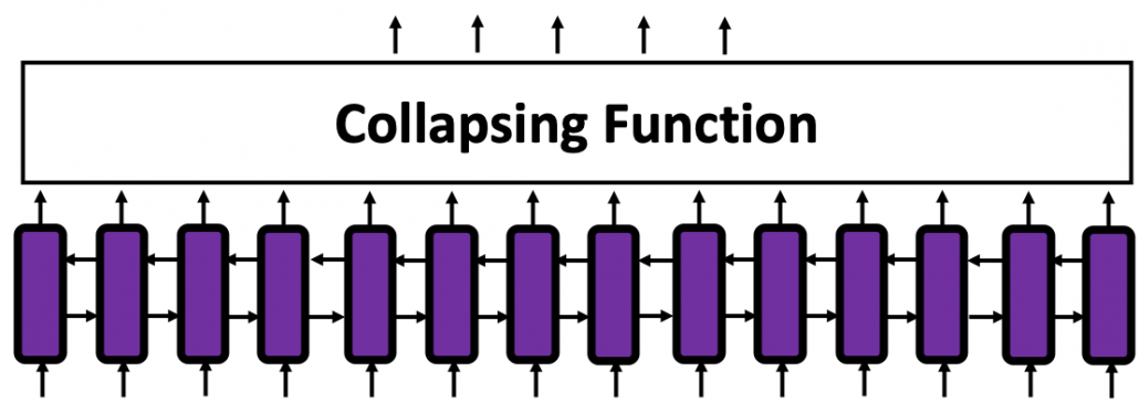
In many situations, RNNs are simplified as below. If you have read through this article until this point, I bet you gained some better understanding of RNNs, so you should little by little get used to this more abstract, blackboxed way of showing RNN.

You have seen that you can unfold an RNN, per time step. From now on I am going to show the simple RNN in a simpler way, based on the MIT textbook which I recomment. The figure below shows how RNN propagate forward during two time steps $(t-1), (t)$ .

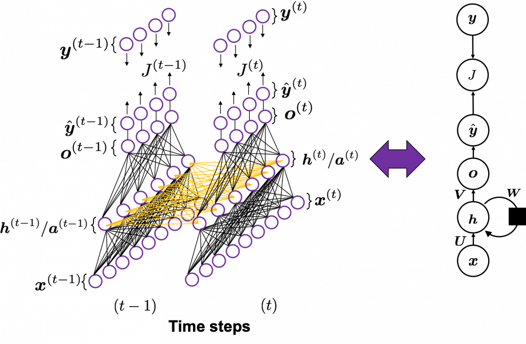
The input $\boldsymbol{x}^{(t-1)}$ at time step $(t-1)$ propagate forward as a normal DCL, and gives out the output $\hat{\boldsymbol{y}} ^{(t)}$ (The notation on the $\boldsymbol{y} ^{(t)}$ is called “hat,” and it means that the value is an estimated value. Whatever machine learning tasks you work on, the outputs of the functions are just estimations of ideal outcomes. You need to adjust parameters for better estimations. You should always be careful whether it is an actual value or an estimated value in the context of machine learning or statistics). But the most important parts are the middle layers.

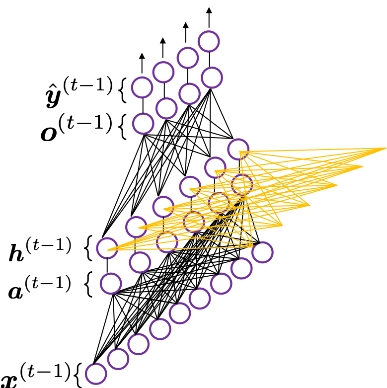
*To be exact I should have drawn the middle layers as connections of two layers of neurons like the figure at the right side. But I made my figure closer to the chart in the MIT textbook, and also most other study materials show the combinations of the two neurons before/after activation as one neuron.

$\boldsymbol{a}^{(t)}$ is just linear summations of $\boldsymbol{x}^{(t)}$ (If you do not know what “linear summations” mean, please scroll this page a bit), and $\boldsymbol{h}^{(t)}$ is a combination of activated values of $\boldsymbol{a}^{(t)}$ and linear summations of $\boldsymbol{h}^{(t-1)}$ from the last time step, with recurrent connections. The values of $\boldsymbol{h}^{(t)}$ propagate forward in two ways. One is normal DCL forward propagation to $\hat{\boldsymbol{y}} ^{(t)}$ and $\boldsymbol{o}^{(t)}$ , and the other is recurrent connections to $\boldsymbol{h}^{(t+1)}$ .

These are equations for each step of forward propagation.

$\boldsymbol{a}^{(t)} = \boldsymbol{b} + \boldsymbol{W} \cdot \boldsymbol{h}^{(t-1)} + \boldsymbol{U} \cdot \boldsymbol{x}^{(t)}$
$\boldsymbol{h}^{(t)}= g(\boldsymbol{a}^{(t)})$
$\boldsymbol{o}^{(t)} = \boldsymbol{c} + \boldsymbol{V} \cdot \boldsymbol{h}^{(t)}$
$\hat{\boldsymbol{y}} ^{(t)} = f(\boldsymbol{o}^{(t)})$

*Please forgive me for adding some mathematical equations on this article even though I pledged not to in the first article. You can skip the them, but for some people it is on the contrary more confusing if there are no equations. In case you are allergic to mathematics, I prescribed some treatments below.

*Linear summation is a type of weighted summation of some elements. Concretely, when you have a vector $\boldsymbol{x}=(x_0, x_1, x_2)$ , and weights $\boldsymbol{w}=(w_0,w_1, w_2)$ , then $\boldsymbol{w}^T \cdot \boldsymbol{x} = w_0 \cdot x_0 + w_1 \cdot x_1 +w_2 \cdot x_2$ is a linear summation of $\boldsymbol{x}$ , and its weights are $\boldsymbol{w}$ .

*When you see a product of a matrix and a vector, for example a product of $\boldsymbol{W}$ and $\boldsymbol{v}$ , you should clearly make an image of connections between two layers of a neural network. You can also say each element of $\boldsymbol{u}}$ is a linear summations all the elements of $\boldsymbol{v}}$ , and $\boldsymbol{W}$ gives the weights for the summations.

A very important point is that you share the same parameters, in this case $\boldsymbol{\theta \in \{\boldsymbol{U}, \boldsymbol{W}, \boldsymbol{b}, \boldsymbol{V}, \boldsymbol{c} \}}$ , at every time step.

And you are likely to see this RNN in this blackboxed form.

3, The steps of back propagation of simple RNN

In the last article, I said “I have to say backprop of RNN, especially LSTM (a useful and mainstream type or RNN), is a monster of chain rules.” I did my best to make my PowerPoint on LSTM backprop straightforward. But looking at it again, the LSTM backprop part still looks like an electronic circuit, and it requires some patience from you to understand it. If you want to understand LSTM at a more mathematical level, understanding the flow of simple RNN backprop is indispensable, so I would like you to be patient while understanding this step (and you have to be even more patient while understanding LSTM backprop).

This might be a matter of my literacy, but explanations on RNN backprop are very frustrating for me in the points below.

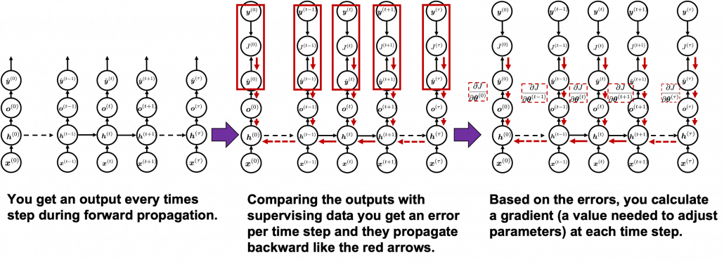
Most explanations just show how to calculate gradients at each time step.
Most study materials are visually very poor.
Most explanations just emphasize that “errors are back propagating through time,” using tons of arrows, but they lack concrete instructions on how actually you renew parameters with those errors.

If you can relate to the feelings I mentioned above, the instructions from now on could somewhat help you. And with the animated PowerPoint slide I prepared, you would have clear understandings on this topic at a more mathematical level.

Backprop of RNN , as long as you are thinking about simple RNNs, is not so different from that of DCLs. But you have to be careful about the meaning of errors in the context of RNN backprop. Back propagation through time (BPTT) is one of the major methods for RNN backprop, and I am sure most textbooks explain BPTT. But most study materials just emphasize that you need errors from all the time steps, and I think that is very misleading and confusing.

You need all the gradients to adjust parameters, but you do not necessarily need all the errors to calculate those gradients. Gradients in the context of machine learning mean partial derivatives of error functions (in this case $J$ ) with respect to certain parameters, and mathematically a gradient of $J$ with respect to $\boldsymbol{\theta \in \{\boldsymbol{U}, \boldsymbol{W}, \boldsymbol{b}^{(t)}, \boldsymbol{V}, \boldsymbol{c} \}}$ is denoted as $( \frac{\partial J}{\partial \boldsymbol{\theta}} )$ . And another confusing point in many textbooks, including the MIT one, is that they give an impression that parameters depend on time steps. For example some study materials use notations like $\frac{\partial J}{\partial \boldsymbol{\theta}^{(t)}}$ , and I think this gives an impression that this is a gradient with respect to the parameters at time step $(t)$ . In my opinion this gradient rather should be written as $( \frac{\partial J}{\partial \boldsymbol{\theta}} )^{(t)}$ . But many study materials denote gradients of those errors in the former way, so from now on let me use the notations which you can see in the figures in this article.

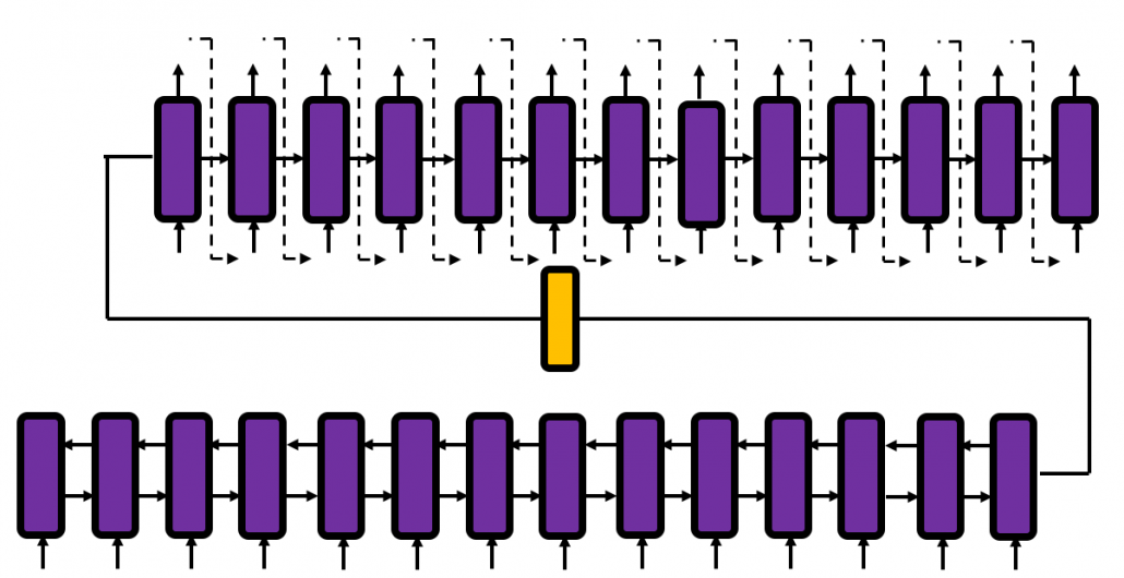
In order to calculate the gradient $\frac{\partial J}{\partial \boldsymbol{x}^{(t)}}$ you need errors from time steps $s (s \geq t) \quad$ (as you can see in the figure, in order to calculate a gradient in a colored frame, you need all the errors in the same color).

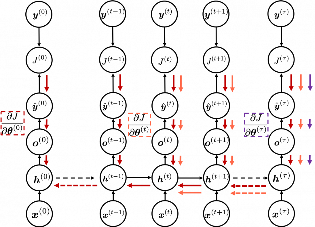
*To be exact, in the figure above I am supposed prepare much more arrows in $\tau + 1$ different colors to show the whole process of RNN backprop, but that is not realistic. In the figure I displayed only the flows of errors necessary for calculating each gradient at time step $0, t, \tau$ .

*Another confusing point is that the $\frac{\partial J}{\partial \boldsymbol{\ast ^{(t)}}}, \boldsymbol{\ast} \in \{\boldsymbol{a}^{(t)}, \boldsymbol{h}^{(t)}, \boldsymbol{o}^{(t)}, \dots \}$ are correct notations, because $\boldsymbol{\ast}$ are values of neurons after forward propagation. They depend on time steps, and these are very values which I have been calling “errors.” That is why parameters do not depend on time steps, whereas errors depend on time steps.

As I mentioned before, you share the same parameters at every time step. Again, please do not assume that parameters are different from time step to time step. It is gradients/errors (you need errors to calculate gradients) which depend on time step. And after calculating errors at every time step, you can finally adjust parameters one time, and that’s why this is called “back propagation through time.” (It is easy to imagine that this method can be very inefficient. If the input is the whole text on a Wikipedia link, you need to input all the sentences in the Wikipedia text to renew parameters one time. To solve this problem there is a backprop method named “truncated BPTT,” with which you renew parameters based on a part of a text. )

And after calculating those gradients $\frac{\partial J}{\partial \boldsymbol{\theta}^{(t)}}$ you can take a summation of them: $\frac{\partial J}{\partial \boldsymbol{\theta}}=\sum_{t=0}^{t=\tau}{\frac{\partial J}{\partial \boldsymbol{\theta}^{(t)}}}$ . With this gradient $\frac{\partial J}{\partial \boldsymbol{\theta}}$ , you can finally renew the value of $\boldsymbol{\theta}$ one time.

At the beginning of this article I mentioned that simple RNNs are no longer for practical uses, and that comes from exploding/vanishing problem of RNN. This problem was one of the reasons for the AI winter which lasted for some 20 years. In the next article I am going to write about LSTM, a fancier type of RNN, in the context of a history of neural network history.

* I make study materials on machine learning, sponsored by DATANOMIQ. I do my best to make my content as straightforward but as precise as possible. I include all of my reference sources. If you notice any mistakes in my materials, including grammatical errors, please let me know (email: yasuto.tamura@datanomiq.de). And if you have any advice for making my materials more understandable to learners, I would appreciate hearing it.

Interview – Machine Learning in Marketing und CRM

June 11, 2020/in Artificial Intelligence, Data Science, Data Science News, Gerneral, Insights, Interviews, Machine Learning, Main Category/by Redaktion

Interview mit Herrn Laurenz Wuttke von der datasolut GmbH über Machine Learning in Marketing und CRM.

Laurenz Wuttke ist Data Scientist und Gründer der datasolut GmbH. Er studierte Wirtschaftsinformatik an der Hochschule Hannover und befasst sich bereits seit 2011 mit Marketing- bzw. CRM-Systemen und der Datenanalyse. Heute ist er Dozent für Big Data im Marketing an der Hochschule Düsseldorf und unterstützt Unternehmen dabei, durch den Einsatz von künstlicher Intelligenz, individuell auf die Kundenbedürfnisse tausender Kunden einzugehen. Damit jeder Marketing Manager jedem Kunden das richtige Angebot zur richtigen Zeit machen kann.

Data Science Blog: Herr Wuttke, Marketing gilt als einer der Pionier-Bereiche der Unternehmen für den Einstieg in Big Data Analytics. Wie etabliert ist Big Data und Data Science heute im Marketing?

Viele Unternehmen in Deutschland erkennen gerade Chancen und den Wert ihrer Daten. Dadurch investieren die Unternehmen in Big Data Infrastruktur und Data Science Teams.

Gleichzeitig denke ich, wir stehen im Marketing gerade am Anfang einer neuen Daten-Ära. Big Data und Data Science sind im Moment noch ein Thema der großen Konzerne. Viele kleine und mittelständische Unternehmen haben noch viele offene Potentiale in Bezug auf intelligente Kundenanalysen.

Durch stetig steigende Preise für die Kundenakquise, wird die Erhaltung und Steigerung einer guten Kundenbindung immer wichtiger. Und genau hier sehe ich die Vorteile durch Data Science im Marketing. Unternehmen können viel genauer auf Kundenbedürfnisse eingehen, antizipieren welches Produkt als nächstes gekauft wird und so ihr Marketing zielgenau ausrichten. Dieses „personalisierte Marketing“ führt zu einer deutlich stärkeren Kundenbindung und steigert langfristig Umsätze.

Viele amerikanische Unternehmen machen es vor, aber auch deutsche Unternehmen wie Zalando oder AboutYou investieren viel Geld in die Personalisierung ihres Marketings. Ich denke, die Erfolge sprechen für sich.

Data Science Blog: Ein häufiges Anliegen für viele Marketing Manager ist die treffsichere Kundensegmentierung nach vielerlei Kriterien. Welche Verbesserungen sind hier möglich und wie können Unternehmen diese erreichen?

Kundensegmentierungen sind ein wichtiger Bestandteil vieler Marketingstrategien. Allerdings kann man hier deutlich weitergehen und Marketing im Sinne von „Segments of One“ betreiben. Das bedeutet wir haben für jeden einzelnen Kunden eine individuelle „Next Best Action und Next Best Offer“.

Somit wird jeder Kunde aus Sicht des Marketings individuell betrachtet und bekommt individuelle Produktempfehlungen sowie Marketingmaßnahmen, welche auf das jeweilige Kundenbedürfnis zugeschnitten sind.

Dies ist auch ein wichtiger Schritt für die Marketingautomatisierung, denn wir können im Marketing schlichtweg keine tausenden von Kunden persönlich betreuen.

Data Science Blog: Sind die Kundencluster dann erkannt, stellt sich die Frage, wie diese besser angesprochen werden können. Wie funktioniert die dafür notwendige Kundenanalyse?

Ganz unterschiedlich, je nach Geschäftsmodell und Branche fällt die Kundenanalyse anders aus. Wir schauen uns unterschiedliche Merkmale zum historischen Kaufverhalten, Demografie und Produktnutzung an. Daraus ergeben sich in der Regel sehr schnell Kundenprofile oder Personas, die gezielt angesprochen werden können.

Data Science Blog: Oft werden derartige Analyse-Vorhaben auf Grund der Befürchtung, die relevanten Daten seien nicht verfügbar oder die Datenqualität sei einer solchen Analyse nicht würdig, gar nicht erst gestartet. Sind das begründete Bedenken?

Nein, denn oft kommen die Daten, die für eine Kundenanalyse oder die Vorhersage von Ergebnissen braucht, aus Datenquellen wie z.B. den Transaktionsdaten. Diese Daten hat jedes Unternehmen in guter Qualität vorliegen.

Natürlich werden die Analysen besser, wenn weitere Datenquellen wie bspw. Produktmetadaten, Kundeneigenschaften oder das Klickverhalten zur Verfügung stehen, aber es ist kein Muss.

Aus meiner Praxiserfahrung kann ich sagen, dass hier oft ungenutzte Potentiale schlummern.

Data Science Blog: Wie ist da eigentlich Ihre Erfahrung bzgl. der Interaktion zwischen Marketing und Business Intelligence? Sollten Marketing Manager ihre eigenen Datenexperten haben oder ist es besser, diese Ressourcen zentral in einer BI-Abteilung zu konzentrieren?

Aus meiner Sicht funktioniert moderenes Marketing heute nicht mehr ohne valide Datenbasis. Aus diesem Grund ist die Zusammenarbeit von Marketing und Business Intelligence unersetzbar, besonders wenn es um Bestandskundenmarketing geht. Hier laufen idealerweise alle Datenquellen in einer 360 Grad Kundensicht zusammen.

Dies kann dann auch als die Datenquelle für Machine Learning und Data Science verwendet werden. Alle wichtigen Daten können aus einer strukturierten 360 Grad Sicht zu einer Machine Learning Datenbasis (ML-Feature Store) umgewandelt werden. Das spart enorm viel Zeit und viel Geld.

Zu Ihrer zweiten Frage: Ich denke es gibt Argumente für beide Konstrukte, daher habe ich da keine klare Präferenz. Mir ist immer wichtig, dass der fachliche Austausch zwischen Technik und Fachbereich gut funktioniert. Ziele müssen besprochen und gegeben falls angepasst werden, um immer in die richtige Richtung zu gehen. Wenn diese Voraussetzung mit einer guten Data Science Infrastruktur gegeben ist, wird Data Science für wirklich skalierbar.

Data Science Blog: Benötigen Unternehmen dafür eine Customer Data Platform (CDP) oder zumindest ein CRM? Womit sollten Unternehmen beginnen, sollten sie noch ganz am Anfang stehen?

Eine Customer Data Platform (CDP) ist von Vorteil, ist aber kein Muss für den Anfang. Ein guts CRM-System oder gute gepflegte Kundendatenbank reicht zunächst für den Anfang.

Natürlich bietet eine CDP einen entscheidenden Vorteil durch die Zusammenführung von der Online- und der CRM-Welt. Das Klickverhalten hat einen enormen Einfluss auf die analytischen Modelle und hilft dabei, Kunden immer besser zu verstehen. Das ist besonders wichtig in unserer Zeit, da wir immer weniger direkten Kundenkontakt haben und zukünftig wird dieser auch noch weiter abnehmen.

Zusammengefasst: Wer diese Kundendaten intelligent miteinander verknüpft hat einen großen Vorteil.

Data Science Blog: Wie integrieren Sie App- und Webtracking in Ihre Analysen?

Trackingdaten aus Apps und Webseiten sind ein wichtiger Bestandteil unserer Machine Learning Modelle. Sie geben wichtige Informationen über das Kundenverhalten preis. So können die Trackingdaten gute Merkmale für Anwendungsfälle wie Churn Prediction, Customer Lifetime Value und Next Best Offer sein.

Häufig sind die Trackingdaten von unterschiedlichen Anbietern (Google Analytics, Piwik etc.) leicht anders in ihrer Struktur, dafür haben wir uns einen intelligenten Ansatz überlegt, um diese zu vereinheitlichen und in unseren Modellen anzuwenden.

Data Science Blog: Zurück zum Kunden. Seine Bedürfnisse stehen bei erfolgreichen Unternehmen im Fokus stehen. Einige Geschäftsmodelle basieren auf Abonnements oder Mitgliedschaften. Wie können Sie solchen Unternehmen helfen?

Abonnements und Subscriptions sind ein großer Trend: Der Kunde wird zum Nutzer und es fallen viele Kundendaten an, die gesammelt werden können. Viele unserer Kunden haben subscription- oder vertragsbasierte Geschäftsmodelle, was ich persönlich sehr interessante Geschäftsmodelle finde.

Diese haben häufig die Herausforderung ihre Kunden langfristig zu binden und eine gesunde Kundenbindung aufzubauen. Die Akquisition ist meistens sehr teuer und die Kundenabwanderung oder Customer Churn zu reduzieren damit ein strategisches Ziel. Wirklich erfolgreich werden diese dann, wenn die Churn Rate geringgehalten wird.

Die Lösung für eine niedrige Kundenabwanderung, neben einem guten Produkt und gutem Kundenservice, ist eine Churn Prediction und darauf aufbauende Churn Prevention Maßnahmen. Wir nehmen uns dazu das historische Kundenverhalten, schauen uns die Kündiger an und modellieren daraus eine Vorhersage für die Kundenabwanderung. So können Unternehmen abwanderungsgefährdete Kunden schon frühzeitig erkennen und entsprechend handeln. Das hat den entscheidenden Vorteil, dass man nicht einen schon verlorenen Kunden erneut gewinnen muss.

Es gibt aber auch Möglichkeiten schon weit vor der eigentlichen Churn-Gefahr anzusetzen, bei drohender Inaktivität. So haben wir für einen großen Fitness-App-Anbieter ein Alarmsystem entwickelt, das Kunden automatisiert Engagement-Kampagnen versendet, um bei drohender Inaktivität, den Kunden auf die Angebote aufmerksam zu machen. Sie kennen das von der Netflix-App, welche Ihnen jeden Abend einen guten Tipp für das Fernsehprogramm bereitstellt.

Data Science Blog: Gehen wir mal eine Ebene höher. So mancher CMO hat mit dem CFO den Deal, jährlich nur einen bestimmten Betrag ins Marketing zu stecken. Wie hilft Data Science bei der Budget-Verteilung auf die Bestandskunden?

Da gibt es eine einfache Lösung für „Customer Lifetime Value Prognosen“. Durch Machine Learning wird für jeden einzelnen Kunden eine Umsatz-Vorhersage für einen bestimmten Zeitraum getroffen. So kann das Bestandkundenmarketing das Marketingbudget ganz gezielt einsetzen und nach dem Kundenwert steuern. Ich gebe Ihnen ein Beispiel: Kundenreaktivierung im Handel. Sie haben ein bestimmtes Budget und können nicht jedem Kunden eine Reaktivierungsmaßnahme zukommen lassen. Wenn Sie einen gut berechneten Customer Lifetime Value haben, können Sie sich so auf die wertigen Kunden konzentrieren und diese reaktivieren.

Data Science Blog: Mit welchen Technologien arbeiten Sie bevorzugt? Welche Tools sind gerade im Kontext von analytischen Aufgaben im Marketing besonders effizient?

Wir haben uns in den letzten Jahren besonders auf Python und PySpark fokussiert. Mit der Entwicklung von Python für Data Science konnten die anderen Umgebungen kaum mithalten und somit ist Python aus meiner Sicht derzeit die beste Umgebung für unsere Lösungen.

Auch die Cloud spielt eine große Rolle für uns. Als kleines Unternehmen haben wir uns bei datasolut auf die AWS Cloud fokussiert, da wir gar nicht in der Lage wären, riesige Datenbestände unserer Kunden zu hosten.

Vor allem von dem hohen Automatisierungsgrad in Bezug auf Datenverarbeitung und Machine Learning bietet AWS alles, was das Data Science Herz begehrt.

Data Science Blog: Was würden Sie einem Junior Marketing Manager und einem Junior Data Scientist für den Ausbau seiner Karriere raten? Wie werden diese jungen Menschen zukünftig beruflich erfolgreich?

Dem Junior Marketing Manager würde ich immer raten, dass er sich Datenanalyse-Skills erarbeiten soll. Aber vor allem sollte er verstehen, was mit Daten alles möglich ist und wie diese eingesetzt werden können. Auch in meiner Vorlesung zu „Big Data im Marketing“ an der Hochschule Düsseldorf unterrichte ich Studierende, die auf Marketing spezialisiert sind. Hier gebe ich stets diesen Ratschlag.

Bei den Junior Daten Scientist ist es andersherum. Ich sehe in der Praxis immer wieder Data Scientists, die den Transfer zwischen Marketing und Data Science nicht gut hinbekommen. Daher rate ich jedem Data Scientist, der sich auf Marketing und Vertrieb fokussieren will, dass hier fachliches Know-How essentiell ist. Kein Modell oder Score hat einen Wert für ein Unternehmen, wenn es nicht gut im Marketing eingesetzt wird und dabei hilft, Marketingprozesse zu automatisieren.

Ein weiterer wichtiger Aspekt ist, dass sich Data Science und Machine Learning gerade rasant ändern. Die Automatisierung (Stichwort: AutoML) von diesen Prozessen ist auf der Überholspur, dass zeigen die großen Cloudanbieter ganz deutlich. Auch wir nutzen diese Technologie schon in der Praxis. Was der Algorithmus aber nicht übernehmen kann, ist der Transfer und Enablement der Fachbereiche.

Data Science Blog: Zum Schluss noch eine Bitte: Was ist Ihre Prophezeiung für die kommenden Jahre 2021/2022. What is the next big thing in Marketing Analytics?

Es gibt natürlich viele kleinere Trends, welche das Marketing verändern werden. Ich denke jedoch, dass die größte Veränderung für die Unternehmen sein wird, dass es einen viel großflächigeren Einsatz von Machine Learning im Marketing geben wird. Dadurch wird der Wettbewerb härter und für viele Unternehmen wird Marketing Analytics ein essentieller Erfolgsfaktor sein.

How Text to Speech Voices Are Used In Data Science

June 9, 2020/in Data Science News, Insights, Machine Learning, Main Category/by Walter T. Cassady

To speak on voices, text to speech platforms are bringing versatility to a new scale by implementing voices that sound more personal and less like a robot. As these services gain traction, vocal quality, and implementation improve to give sounds that feel like they’re speaking to you from a human mouth.

The intention of most text to speech platforms have always been to provide experiences that users feel comfortable using. Voices are a huge part of that, so great strides have been taken to ensure that they sound right.

How Voices are Utilized

Voices in the text to speech are generated by a computer itself. As the computer-generated voices transcribe the text into oral responses, they make up what we hear as dialogue read to us. These voice clips initially had the problem of sounding robotic and unpersonable as they were pulled digitally together. Lately, though, the technology has improved to bring faster response time in transcribing words, as well as seamlessly stringing together. This has brought the advantage of making a computer-generated voice sound much more natural and human. As people seek to connect more with the works they read, having a human-sounding voice is a huge step in letting listeners relate to their works.

To give an example of where this works, you might have a GPS in your car. The GPS has a function where it will transcribe the car’s route and tell you each instruction. Some GPS companies have made full use of this feature and added fun voices to help entertain drivers. These include Darth Vader and Yoda from Star Wars or having Morgan Freeman and Homer Simpson narrate your route. Different voice types are utilized in services depending on the situation. Professional uses like customer service centers will keep automated voices sounding professional and courteous when assisting customers. Educational systems will keep softer and kinder sounding voices to help sound more friendly with students.

When compared to older solutions, the rise of vocal variety in Text to Speech services has taken huge leaps as more people see the value of having a voice that they can connect to. Expressive voices and emotional variance are being applied to voices to help further convey this, with happy or sad sounding voices being implemented wherever appropriate. As time goes on, these services will get better at the reading context within sentences to apply emotion and tone at the correct times, and improve overall vocal quality as well. These reinvent past methods by advancing the once static and robotic sounds that used to be commonplace among text to voice services.

More infrastructures adopt these services to expand their reach to consumers who might not have the capabilities to utilize their offerings. Having clear and relatable voices matter because customers and users will be drawn to them considerably more than if they chose not to offer them at all. In the near future text to speech voices will develop even further, enhancing the way people of all kinds connect to the words they read.

Prerequisites for understanding RNN at a more mathematical level

June 1, 2020/in Artificial Intelligence, Big Data, Data Science, Data Science Hack, Deep Learning, Gerneral, Insights, Machine Learning, Main Category, Natural Language Processing, Text Mining/by Yasuto Tamura

Writing the A gentle introduction to the tiresome part of understanding RNN Article Series on recurrent neural network (RNN) is nothing like a creative or ingenious idea. It is quite an ordinary topic. But still I am going to write my own new article on this ordinary topic because I have been frustrated by lack of sufficient explanations on RNN for slow learners like me.

I think many of readers of articles on this website at least know that RNN is a type of neural network used for AI tasks, such as time series prediction, machine translation, and voice recognition. But if you do not understand how RNNs work, especially during its back propagation, this blog series is for you.

After reading this articles series, I think you will be able to understand RNN in more mathematical and abstract ways. But in case some of the readers are allergic or intolerant to mathematics, I tried to use as little mathematics as possible.

Ideal prerequisite knowledge:

Some understanding on densely connected layers (or fully connected layers, multilayer perception) and how their forward/back propagation work.
Some understanding on structure of Convolutional Neural Network.

*In this article “Densely Connected Layers” is written as “DCL,” and “Convolutional Neural Network” as “CNN.”

1, Difficulty of Understanding RNN

I bet a part of difficulty of understanding RNN comes from the variety of its structures. If you search “recurrent neural network” on Google Image or something, you will see what I mean. But that cannot be helped because RNN enables a variety of tasks.

Another major difficulty of understanding RNN is understanding its back propagation algorithm. I think some of you found it hard to understand chain rules in calculating back propagation of densely connected layers, where you have to make the most of linear algebra. And I have to say backprop of RNN, especially LSTM, is a monster of chain rules. I am planing to upload not only a blog post on RNN backprop, but also a presentation slides with animations to make it more understandable, in some external links.

In order to avoid such confusions, I am going to introduce a very simplified type of RNN, which I call a “simple RNN.” The RNN displayed as the head image of this article is a simple RNN.

2, How Neurons are Connected

How to connect neurons and how to activate them is what neural networks are all about. Structures of those neurons are easy to grasp as long as that is about DCL or CNN. But when it comes to the structure of RNN, many study materials try to avoid showing that RNNs are also connections of neurons, as well as DCL or CNN(*If you are not sure how neurons are connected in CNN, this link should be helpful. Draw a random digit in the square at the corner.). In fact the structure of RNN is also the same, and as long as it is a simple RNN, and it is not hard to visualize its structure.

Even though RNN is also connections of neurons, usually most RNN charts are simplified, using blackboxes. In case of simple RNN, most study material would display it as the chart below.

But that also cannot be helped because fancier RNN have more complicated connections of neurons, and there are no longer advantages of displaying RNN as connections of neurons, and you would need to understand RNN in more abstract way, I mean, as you see in most of textbooks.

I am going to explain details of simple RNN in the next article of this series.

3, Neural Networks as Mappings

If you still think that neural networks are something like magical spider webs or models of brain tissues, forget that. They are just ordinary mappings.

If you have been allergic to mathematics in your life, you might have never heard of the word “mapping.” If so, at least please keep it in mind that the equation $y=f(x)$ , which most people would have seen in compulsory education, is a part of mapping. If you get a value x, you get a value y corresponding to the x.

But in case of deep learning, x is a vector or a tensor, and it is denoted in bold like $\boldsymbol{x}$ . If you have never studied linear algebra , imagine that a vector is a column of Excel data (only one column), a matrix is a sheet of Excel data (with some rows and columns), and a tensor is some sheets of Excel data (each sheet does not necessarily contain only one column.)

CNNs are mainly used for image processing, so their inputs are usually image data. Image data are in many cases (3, hight, width) tensors because usually an image has red, blue, green channels, and the image in each channel can be expressed as a height*width matrix (the “height” and the “width” are number of pixels, so they are discrete numbers).

The convolutional part of CNN (which I call “feature extraction part”) maps the tensors to a vector, and the last part is usually DCL, which works as classifier/regressor. At the end of the feature extraction part, you get a vector. I call it a “semantic vector” because the vector has information of “meaning” of the input image. In this link you can see maps of pictures plotted depending on the semantic vector. You can see that even if the pictures are not necessarily close pixelwise, they are close in terms of the “meanings” of the images.

In the example of a dog/cat classifier introduced by François Chollet, the developer of Keras, the CNN maps (3, 150, 150) tensors to 2-dimensional vectors, (1, 0) or (0, 1) for (dog, cat).

Wrapping up the points above, at least you should keep two points in mind: first, DCL is a classifier or a regressor, and CNN is a feature extractor used for image processing. And another important thing is, feature extraction parts of CNNs map images to vectors which are more related to the “meaning” of the image.

Importantly, I would like you to understand RNN this way. An RNN is also just a mapping.

*I recommend you to at least take a look at the beautiful pictures in this link. These pictures give you some insight into how CNN perceive images.

4, Problems of DCL and CNN, and needs for RNN

Taking an example of RNN task should be helpful for this topic. Probably machine translation is the most famous application of RNN, and it is also a good example of showing why DCL and CNN are not proper for some tasks. Its algorithms is out of the scope of this article series, but it would give you a good insight of some features of RNN. I prepared three sentences in German, English, and Japanese, which have the same meaning. Assume that each sentence is divided into some parts as shown below and that each vector corresponds to each part. In machine translation we want to convert a set of the vectors into another set of vectors.

Then let’s see why DCL and CNN are not proper for such task.

The input size is fixed: In case of the dog/cat classifier I have mentioned, even though the sizes of the input images varies, they were first molded into (3, 150, 150) tensors. But in machine translation, usually the length of the input is supposed to be flexible.
The order of inputs does not mater: In case of the dog/cat classifier the last section, even if the input is “cat,” “cat,” “dog” or “dog,” “cat,” “cat” there’s no difference. And in case of DCL, the network is symmetric, so even if you shuffle inputs, as long as you shuffle all of the input data in the same way, the DCL give out the same outcome . And if you have learned at least one foreign language, it is easy to imagine that the orders of vectors in sequence data matter in machine translation.

*It is said English language has phrase structure grammar, on the other hand Japanese language has dependency grammar. In English, the orders of words are important, but in Japanese as long as the particles and conjugations are correct, the orders of words are very flexible. In my impression, German grammar is between them. As long as you put the verb at the second position and the cases of the words are correct, the orders are also relatively flexible.

5, Sequence Data

We can say DCL and CNN are not useful when you want to process sequence data. Sequence data are a type of data which are lists of vectors. And importantly, the orders of the vectors matter. The number of vectors in sequence data is usually called time steps. A simple example of sequence data is meteorological data measured at a spot every ten minutes, for instance temperature, air pressure, wind velocity, humidity. In this case the data is recorded as 4-dimensional vector every ten minutes.

But this “time step” does not necessarily mean “time.” In case of natural language processing (including machine translation), which you I mentioned in the last section, the numberings of each vector denoting each part of sentences are “time steps.”

And RNNs are mappings from a sequence data to another sequence data.

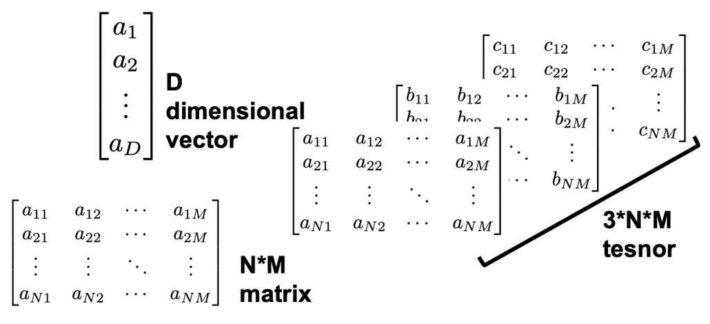
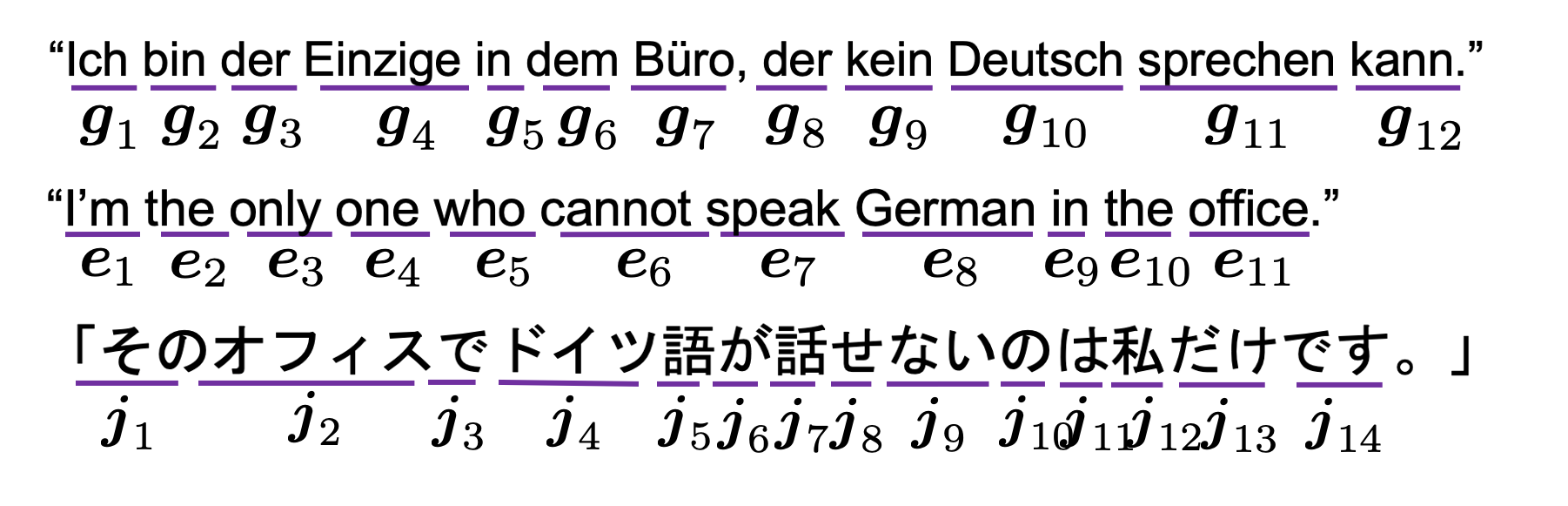
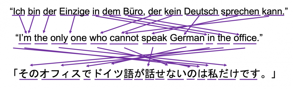
In case of the machine translation above, the each sentence in German, English, and German is expressed as sequence data $\boldsymbol{G}=(\boldsymbol{g}_1,\dots ,\boldsymbol{g}_{12}), \boldsymbol{E}=(\boldsymbol{e}_1,\dots ,\boldsymbol{e}_{11}), \boldsymbol{J}=(\boldsymbol{j}_1,\dots ,\boldsymbol{j}_{14})$ , and machine translation is nothing but mappings between these sequence data.

*At least I found a paper on the RNN’s capability of universal approximation on many-to-one RNN task. But I have not found any papers on universal approximation of many-to-many RNN tasks. Please let me know if you find any clue on whether such approximation is possible. I am desperate to know that.

6, Types of RNN Tasks

RNN tasks can be classified into some types depending on the lengths of input/output sequences (the “length” means the times steps of input/output sequence data).

If you want to predict the temperature in 24 hours, based on several time series data points in the last 96 hours, the task is many-to-one. If you sample data every ten minutes, the input size is 96*6=574 (the input data is a list of 574 vectors), and the output size is 1 (which is a value of temperature). Another example of many-to-one task is sentiment classification. If you want to judge whether a post on SNS is positive or negative, the input size is very flexible (the length of the post varies.) But the output size is one, which is (1, 0) or (0, 1), which denotes (positive, negative).

*The charts in this section are simplified model of RNN used for each task. Please keep it in mind that they are not 100% correct, but I tried to make them as exact as possible compared to those in other study materials.

Music/text generation can be one-to-many tasks. If you give the first sound/word you can generate a phrase.

Next, let’s look at many-to-many tasks. Machine translation and voice recognition are likely to be major examples of many-to-many tasks, but here name entity recognition seems to be a proper choice. Name entity recognition is task of finding proper noun in a sentence . For example if you got two sentences “He said, ‘Teddy bears on sale!’ ” and ‘He said, “Teddy Roosevelt was a great president!” ‘ judging whether the “Teddy” is a proper noun or a normal noun is name entity recognition.

Machine translation and voice recognition, which are more popular, are also many-to-many tasks, but they use more sophisticated models. In case of machine translation, the inputs are sentences in the original language, and the outputs are sentences in another language. When it comes to voice recognition, the input is data of air pressure at several time steps, and the output is the recognized word or sentence. Again, these are out of the scope of this article but I would like to introduce the models briefly.

Machine translation uses a type of RNN named sequence-to-sequence model (which is often called seq2seq model). This model is also very important for other natural language processes tasks in general, such as text summarization. A seq2seq model is divided into the encoder part and the decoder part. The encoder gives out a hidden state vector and it used as the input of the decoder part. And decoder part generates texts, using the output of the last time step as the input of next time step.

Voice recognition is also a famous application of RNN, but it also needs a special type of RNN.

*To be honest, I don’t know what is the state-of-the-art voice recognition algorithm. The example in this article is a combination of RNN and a collapsing function made using Connectionist Temporal Classification (CTC). In this model, the output of RNN is much longer than the recorded words or sentences, so a collapsing function reduces the output into next output with normal length.

You might have noticed that RNNs in the charts above are connected in both directions. Depending on the RNN tasks you need such bidirectional RNNs. I think it is also easy to imagine that such networks are necessary. Again, machine translation is a good example.

And interestingly, image captioning, which enables a computer to describe a picture, is one-to-many-task. As the output is a sentence, it is easy to imagine that the output is “many.” If it is a one-to-many task, the input is supposed to be a vector.

Where does the input come from? I mentioned that the last some layers in of CNN are closely connected to how CNNs extract meanings of pictures. Surprisingly such vectors, which I call a “semantic vectors” is the inputs of image captioning task (after some transformations, depending on the network models).

I think this articles includes major things you need to know as prerequisites when you want to understand RNN at more mathematical level. In the next article, I would like to explain the structure of a simple RNN, and how it forward propagate.

* I make study materials on machine learning, sponsored by DATANOMIQ. I do my best to make my content as straightforward but as precise as possible. I include all of my reference sources. If you notice any mistakes in my materials, please let me know (email: yasuto.tamura@datanomiq.de). And if you have any advice for making my materials more understandable to learners, I would appreciate hearing it.

A gentle introduction to the tiresome part of understanding RNN

May 1, 2020/in Artificial Intelligence, Data Science, Deep Learning, Machine Learning, Mathematics, Uncategorized/by Yasuto Tamura

Just as a normal conversation in a random pub or bar in Berlin, people often ask me “Which language do you use?” I always answer “LaTeX and PowerPoint.”

I have been doing an internship at DATANOMIQ and trying to make straightforward but precise study materials on deep learning. I myself started learning machine learning in April of 2019, and I have been self-studying during this one-year-vacation of mine in Berlin.

Many study materials give good explanations on densely connected layers or convolutional neural networks (CNNs). But when it comes to back propagation of CNN and recurrent neural networks (RNNs), I think there’s much room for improvement to make the topic understandable to learners.

Many study materials avoid the points I want to understand, and that was as frustrating to me as listening to answers to questions in the Japanese Diet, or listening to speeches from the current Japanese minister of the environment. With the slightest common sense, you would always get the feeling “How?” after reading an RNN chapter in any book.

This blog series focuses on the introductory level of recurrent neural networks. By “introductory”, I mean prerequisites for a better and more mathematical understanding of RNN algorithms.

I am going to keep these posts as visual as possible, avoiding equations, but I am also going to attach some links to check more precise mathematical explanations.

This blog series is composed of five contents.:

Interview – IT-Netzwerk Werke überwachen und optimieren mit Data Analytics

April 10, 2020/in Big Data, Data Mining, Data Science, Data Science News, Gerneral, Insights, Interview mit CIO, Interviews, Machine Learning, Use Cases/by Benjamin Aunkofer

Interview mit Gregory Blepp von NetDescribe über Data Analytics zur Überwachung und Optimierung von IT-Netzwerken

Gregory Blepp ist Managing Director der NetDescribe GmbH mit Sitz in Oberhaching im Süden von München. Er befasst sich mit seinem Team aus Consultants, Data Scientists und IT-Netzwerk-Experten mit der technischen Analyse von IT-Netzwerken und der Automatisierung der Analyse über Applikationen.

Data Science Blog: Herr Blepp, der Name Ihres Unternehmens NetDescribe beschreibt tatsächlich selbstsprechend wofür Sie stehen: die Analyse von technischen Netzwerken. Wo entsteht hier der Bedarf für diesen Service und welche Lösung haben Sie dafür parat?

Unsere Kunden müssen nahezu in Echtzeit eine Visibilität über die Leistungsfähigkeit ihrer Unternehmens-IT haben. Dazu gehört der aktuelle Status der Netzwerke genauso wie andere Bereiche, also Server, Applikationen, Storage und natürlich die Web-Infrastruktur sowie Security.

Im Bankenumfeld sind zum Beispiel die uneingeschränkten WAN Verbindungen für den Handel zwischen den internationalen Börsenplätzen absolut kritisch. Hierfür bieten wir mit StableNetⓇ von InfosimⓇ eine Netzwerk Management Plattform, die in Echtzeit den Zustand der Verbindungen überwacht. Für die unterlagerte Netzwerkplattform (Router, Switch, etc.) konsolidieren wir mit GigamonⓇ das Monitoring.

Für Handelsunternehmen ist die Performance der Plattformen für den Online Shop essentiell. Dazu kommen die hohen Anforderungen an die Sicherheit bei der Übertragung von persönlichen Informationen sowie Kreditkarten. Hierfür nutzen wir SplunkⓇ. Diese Lösung kombiniert in idealer Form die generelle Performance Überwachung mit einem hohen Automatisierungsgrad und bietet dabei wesentliche Unterstützung für die Sicherheitsabteilungen.

Data Science Blog: Geht es den Unternehmen dabei eher um die Sicherheitsaspekte eines Firmennetzwerkes oder um die Performance-Analyse zum Zwecke der Optimierung?

Das hängt von den aktuellen Ansprüchen des Unternehmens ab.
Für viele unserer Kunden standen und stehen zunächst Sicherheitsaspekte im Vordergrund. Im Laufe der Kooperation können wir durch die Etablierung einer konsequenten Performance Analyse aufzeigen, wie eng die Verzahnung der einzelnen Abteilungen ist. Die höhere Visibilität erleichtert Performance Analysen und sie liefert den Sicherheitsabteilung gleichzeitig wichtige Informationen über aktuelle Zustände der Infrastruktur.

Data Science Blog: Haben Sie es dabei mit Big Data – im wörtlichen Sinne – zu tun?

Wir unterscheiden bei Big Data zwischen

dem organischen Wachstum von Unternehmensdaten aufgrund etablierter Prozesse, inklusive dem Angebot von neuen Services und
wirklichem Big Data, z. B. die Anbindung von Produktionsprozessen an die Unternehmens IT, also durch die Digitalisierung initiierte zusätzliche Prozesse in den Unternehmen.

Beide Themen sind für die Kunden eine große Herausforderung. Auf der einen Seite muss die Leistungsfähigkeit der Systeme erweitert und ausgebaut werden, um die zusätzlichen Datenmengen zu verkraften. Auf der anderen Seite haben diese neuen Daten nur dann einen wirklichen Wert, wenn sie richtig interpretiert werden und die Ergebnisse konsequent in die Planung und Steuerung der Unternehmen einfließen.

Wir bei NetDescribe kümmern uns mehrheitlich darum, das Wachstum und die damit notwendigen Anpassungen zu managen und – wenn Sie so wollen – Ordnung in das Datenchaos zu bringen. Konkret verfolgen wir das Ziel den Verantwortlichen der IT, aber auch der gesamten Organisation eine verlässliche Indikation zu geben, wie es der Infrastruktur als Ganzes geht. Dazu gehört es, über die einzelnen Bereiche hinweg, gerne auch Silos genannt, die Daten zu korrelieren und im Zusammenhang darzustellen.

Data Science Blog: Log-Datenanalyse gibt es seit es Log-Dateien gibt. Was hält ein BI-Team davon ab, einen Data Lake zu eröffnen und einfach loszulegen?

Das stimmt absolut, Log-Datenanalyse gibt es seit jeher. Es geht hier schlichtweg um die Relevanz. In der Vergangenheit wurde mit Wireshark bei Bedarf ein Datensatz analysiert um ein Problem zu erkennen und nachzuvollziehen. Heute werden riesige Datenmengen (Logs) im IoT Umfeld permanent aufgenommen um Analysen zu erstellen.

Nach meiner Überzeugung sind drei wesentliche Veränderungen der Treiber für den flächendeckenden Einsatz von modernen Analysewerkzeugen.

Die Inhalte und Korrelationen von Log Dateien aus fast allen Systemen der IT Infrastruktur sind durch die neuen Technologien nahezu in Echtzeit und für größte Datenmengen überhaupt erst möglich. Das hilft in Zeiten der Digitalisierung, wo aktuelle Informationen einen ganz neuen Stellenwert bekommen und damit zu einer hohen Gewichtung der IT führen.
Ein wichtiger Aspekt bei der Aufnahme und Speicherung von Logfiles ist heute, dass ich die Suchkriterien nicht mehr im Vorfeld formulieren muss, um dann die Antworten aus den Datensätzen zu bekommen. Die neuen Technologien erlauben eine völlig freie Abfrage von Informationen über alle Daten hinweg.
Logfiles waren in der Vergangenheit ein Hilfswerkzeug für Spezialisten. Die Information in technischer Form dargestellt, half bei einer Problemlösung – wenn man genau wusste was man sucht. Die aktuellen Lösungen sind darüber hinaus mit einer GUI ausgestattet, die nicht nur modern, sondern auch individuell anpassbar und für Nicht-Techniker verständlich ist. Somit erweitert sich der Anwenderkreis des “Logfile Managers” heute vom Spezialisten im Security und Infrastrukturbereich über Abteilungsverantwortliche und Mitarbeiter bis zur Geschäftsleitung.

Der Data Lake war und ist ein wesentlicher Bestandteil. Wenn wir heute Technologien wie Apache/KafkaⓇ und, als gemanagte Lösung, Confluent für Apache/KafkaⓇ betrachten, wird eine zentrale Datendrehscheibe etabliert, von der alle IT Abteilungen profitieren. Alle Analysten greifen mit Ihren Werkzeugen auf die gleiche Datenbasis zu. Somit werden die Rohdaten nur einmal erhoben und allen Tools gleichermaßen zur Verfügung gestellt.

Data Science Blog: Damit sind Sie ein Unternehmen das Datenanalyse, Visualisierung und Monitoring verbindet, dies jedoch auch mit der IT-Security. Was ist Unternehmen hierbei eigentlich besonders wichtig?

Sicherheit ist natürlich ganz oben auf die Liste zu setzen. Organisation sind naturgemäß sehr sensibel und aktuelle Medienberichte zu Themen wie Cyber Attacks, Hacking etc. zeigen große Wirkung und lösen Aktionen aus. Dazu kommen Compliance Vorgaben, die je nach Branche schneller und kompromissloser umgesetzt werden.

Die NetDescribe ist spezialisiert darauf den Bogen etwas weiter zu spannen.

Natürlich ist die sogenannte Nord-Süd-Bedrohung, also der Angriff von außen auf die Struktur erheblich und die IT-Security muss bestmöglich schützen. Dazu dienen die Firewalls, der klassische Virenschutz etc. und Technologien wie Extrahop, die durch konsequente Überwachung und Aktualisierung der Signaturen zum Schutz der Unternehmen beitragen.

Genauso wichtig ist aber die Einbindung der unterlagerten Strukturen wie das Netzwerk. Ein Angriff auf eine Organisation, egal von wo aus initiiert, wird immer über einen Router transportiert, der den Datensatz weiterleitet. Egal ob aus einer Cloud- oder traditionellen Umgebung und egal ob virtuell oder nicht. Hier setzen wir an, indem wir etablierte Technologien wie zum Beispiel ´flow` mit speziell von uns entwickelten Software Modulen – sogenannten NetDescibe Apps – nutzen, um diese Datensätze an SplunkⓇ, StableNetⓇ weiterzuleiten. Dadurch entsteht eine wesentlich erweiterte Analysemöglichkeit von Bedrohungsszenarien, verbunden mit der Möglichkeit eine unternehmensweite Optimierung zu etablieren.

Data Science Blog: Sie analysieren nicht nur ad-hoc, sondern befassen sich mit der Formulierung von Lösungen als Applikation (App).

Das stimmt. Alle von uns eingesetzten Technologien haben ihre Schwerpunkte und sind nach unserer Auffassung führend in ihren Bereichen. InfosimⓇ im Netzwerk, speziell bei den Verbindungen, VIAVI in der Paketanalyse und bei flows, SplunkⓇ im Securitybereich und Confluent für Apache/KafkaⓇ als zentrale Datendrehscheibe. Also jede Lösung hat für sich alleine schon ihre Daseinsberechtigung in den Organisationen. Die NetDescribe hat es sich seit über einem Jahr zur Aufgabe gemacht, diese Technologien zu verbinden um einen “Stack” zu bilden.

Konkret: Gigaflow von VIAVI ist die wohl höchst skalierbare Softwarelösung um Netzwerkdaten in größten Mengen schnell und und verlustfrei zu speichern und zu analysieren. SplunkⓇ hat sich mittlerweile zu einem Standardwerkzeug entwickelt, um Datenanalyse zu betreiben und die Darstellung für ein großes Auditorium zu liefern.

NetDescribe hat jetzt eine App vorgestellt, welche die NetFlow-Daten in korrelierter Form aus Gigaflow, an SplunkⓇ liefert. Ebenso können aus SplunkⓇ Abfragen zu bestimmten Datensätzen direkt an die Gigaflow Lösung gestellt werden. Das Ergebnis ist eine wesentlich erweiterte SplunkⓇ-Plattform, nämlich um das komplette Netzwerk mit nur einem Knopfdruck (!!!).
Dazu schont diese Anbindung in erheblichem Umfang SplunkⓇ Ressourcen.

Dazu kommt jetzt eine NetDescribe StableNetⓇ App. Weitere Anbindungen sind in der Planung.

Das Ziel ist hier ganz pragmatisch – wenn sich SplunkⓇ als die Plattform für Sicherheitsanalysen und für das Data Framework allgemein in den Unternehmen etabliert, dann unterstützen wir das als NetDescribe dahingehend, dass wir die anderen unternehmenskritischen Lösungen der Abteilungen an diese Plattform anbinden, bzw. Datenintegration gewährleisten. Das erwarten auch unsere Kunden.

Data Science Blog: Auf welche Technologien setzen Sie dabei softwareseitig?

Wie gerade erwähnt, ist SplunkⓇ eine Plattform, die sich in den meisten Unternehmen etabliert hat. Wir machen SplunkⓇ jetzt seit über 10 Jahren und etablieren die Lösung bei unseren Kunden.

SplunkⓇ hat den großen Vorteil dass unsere Kunden mit einem dedizierten und überschaubaren Anwendung beginnen können, die Technologie selbst aber nahezu unbegrenzt skaliert. Das gilt für Security genauso wie Infrastruktur, Applikationsmonitoring und Entwicklungsumgebungen. Aus den ständig wachsenden Anforderungen unserer Kunden ergeben sich dann sehr schnell weiterführende Gespräche, um zusätzliche Einsatzszenarien zu entwickeln.

Neben SplunkⓇ setzen wir für das Netzwerkmanagement auf StableNetⓇ von InfosimⓇ, ebenfalls seit über 10 Jahren schon. Auch hier, die Erfahrungen des Herstellers im Provider Umfeld erlauben uns bei unseren Kunden eine hochskalierbare Lösung zu etablieren.

Confluent für Apache/KafkaⓇ ist eine vergleichbar jüngere Lösung, die aber in den Unternehmen gerade eine extrem große Aufmerksamkeit bekommt. Die Etablierung einer zentralen Datendrehscheibe für Analyse, Auswertungen, usw., auf der alle Daten zur Performance zentral zur Verfügung gestellt werden, wird es den Administratoren, aber auch Planern und Analysten künftig erleichtern, aussagekräftige Daten zu liefern. Die Verbindung aus OpenSource und gemanagter Lösung trifft hier genau die Zielvorstellung der Kunden und scheinbar auch den Zahn der Zeit. Vergleichbar mit den Linux Derivaten von Red Hat Linux und SUSE.

VIAVI Gigaflow hatte ich für Netzwerkanalyse schon erwähnt. Hier wird in den kommenden Wochen mit der neuen Version der VIAVI Apex Software ein Scoring für Netzwerke etabliert. Stellen sie sich den MOS score von VoIP für Unternehmensnetze vor. Das trifft es sehr gut. Damit erhalten auch wenig spezialisierte Administratoren die Möglichkeit mit nur 3 (!!!) Mausklicks konkrete Aussagen über den Zustand der Netzwerkinfrastruktur, bzw. auftretende Probleme zu machen. Ist es das Netz? Ist es die Applikation? Ist es der Server? – der das Problem verursacht. Das ist eine wesentliche Eindämmung des derzeitigen Ping-Pong zwischen den Abteilungen, von denen oft nur die Aussage kommt, “bei uns ist alles ok”.

Abgerundet wird unser Software Portfolio durch die Lösung SentinelOne für Endpoint Protection.

Data Science Blog: Inwieweit spielt Künstliche Intelligenz (KI) bzw. Machine Learning eine Rolle?

Machine Learning spielt heute schon ein ganz wesentliche Rolle. Durch konsequentes Einspeisen der Rohdaten und durch gezielte Algorithmen können mit der Zeit bessere Analysen der Historie und komplexe Zusammenhänge aufbereitet werden. Hinzu kommt, dass so auch die Genauigkeit der Prognosen für die Zukunft immens verbessert werden können.

Als konkretes Beispiel bietet sich die eben erwähnte Endpoint Protection von SentinelOne an. Durch die Verwendung von KI zur Überwachung und Steuerung des Zugriffs auf jedes IoT-Gerät, befähigt SentinelOne Maschinen, Probleme zu lösen, die bisher nicht in größerem Maßstab gelöst werden konnten.

Hier kommt auch unser ganzheitlicher Ansatz zum Tragen, nicht nur einzelne Bereiche der IT, sondern die unternehmensweite IT ins Visier zu nehmen.

Data Science Blog: Mit was für Menschen arbeiten Sie in Ihrem Team? Sind das eher die introvertierten Nerds und Hacker oder extrovertierte Consultants? Was zeichnet Sie als Team fachlich aus?

Nerds und Hacker würde ich unsere Mitarbeiter im technischen Consulting definitiv nicht nennen.

Unser Consulting Team besteht derzeit aus neun Leuten. Jeder ist ausgewiesener Experte für bestimmte Produkte. Natürlich ist es auch bei uns so, dass wir introvertierte Kollegen haben, die zunächst lieber in Abgeschiedenheit oder Ruhe ein Problem analysieren, um dann eine Lösung zu generieren. Mehrheitlich sind unsere technischen Kollegen aber stets in enger Abstimmung mit dem Kunden.

Für den Einsatz beim Kunden ist es sehr wichtig, dass man nicht nur fachlich die Nase vorn hat, sondern dass man auch kommunikationsstark und extrem teamfähig ist. Eine schnelle Anpassung an die verschiedenen Arbeitsumgebungen und “Kollegen” bei den Kunden zeichnet unsere Leute aus.

Als ständig verfügbares Kommunikationstool nutzen wir einen internen Chat der allen jederzeit zur Verfügung steht, so dass unser Consulting Team auch beim Kunden immer Kontakt zu den Kollegen hat. Das hat den großen Vorteil, dass das gesamte Know-how sozusagen “im Pool” verfügbar ist.

Neben den Consultants gibt es unser Sales Team mit derzeit vier Mitarbeitern*innen. Diese Kollegen*innen sind natürlich immer unter Strom, so wie sich das für den Vertrieb gehört.
Dedizierte PreSales Consultants sind bei uns die technische Speerspitze für die Aufnahme und das Verständnis der Anforderungen. Eine enge Zusammenarbeit mit dem eigentlichen Consulting Team ist dann die Voraussetzung für die vorausschauende Planung aller Projekte.

Wir suchen übrigens laufend qualifizierte Kollegen*innen. Details zu unseren Stellenangeboten finden Ihre Leser*innen auf unserer Website unter dem Menüpunkt “Karriere”. Wir freuen uns über jede/n Interessenten*in.

Über NetDescribe:

NetDescribe steht mit dem Claim Trusted Performance für ausfallsichere Geschäftsprozesse und Cloud-Anwendungen. Die Stärke von NetDescribe sind maßgeschneiderte Technologie Stacks bestehend aus Lösungen mehrerer Hersteller. Diese werden durch selbst entwickelte Apps ergänzt und verschmolzen.

Das ganzheitliche Portfolio bietet Datenanalyse und -visualisierung, Lösungskonzepte, Entwicklung, Implementierung und Support. Als Trusted Advisor für Großunternehmen und öffentliche Institutionen realisiert NetDescribe hochskalierbare Lösungen mit State-of-the-Art-Technologien für dynamisches und transparentes Monitoring in Echtzeit. Damit erhalten Kunden jederzeit Einblicke in die Bereiche Security, Cloud, IoT und Industrie 4.0. Sie können agile Entscheidungen treffen, interne und externe Compliance sichern und effizientes Risikomanagement betreiben. Das ist Trusted Performance by NetDescribe.

CAPTCHAs lösen via Maschine Learning

March 9, 2020/in Artificial Intelligence, Data Science, Deep Learning, Insights, Machine Learning, Main Category/by Pavel Shipilov

Wie weit ist das maschinelle Lernen auf dem Gebiet der CAPTCHA-Lösung fortgeschritten?

Maschinelles Lernen ist mehr als ein Buzzword, denn unter der Haube stecken viele Algorithemen, die eine ganze Reihe von Problemen lösen können. Die Lösung von CAPTCHA ist dabei nur eine von vielen Aufgaben, die Machine Learning bewältigen kann. Durch die Arbeit an ein paar Problemen im Zusammenhang mit dem konvolutionellen neuronalen Netz haben wir festgestellt, dass es in diesem Bereich noch viel Verbesserungspotenzial gibt. Die Genauigkeit der Erkennung ist oftmals noch nicht gut genug. Schauen wir uns im Einzelnen an, welche Dienste wir haben, um dieses Problem anzugehen, und welche sich dabei als die besten erweisen.

Was ist CAPTCHA?

CAPTCHA ist kein fremder Begriff mehr für Web-Benutzer. Es handelt sich um die ärgerliche menschliche Validierungsprüfung, die auf vielen Websites hinzugefügt wird. Es ist ein Akronym für Completely Automated Public Turing test for tell Computer and Humans Apart. CAPTCHA kann als ein Computerprogramm bezeichnet werden, das dazu entwickelt wurde, Mensch und Maschine zu unterscheiden, um jede Art von illegaler Aktivität auf Websites zu verhindern. Der Sinn von CAPTCHA ist, dass nur ein Mensch diesen Test bestehen können sollte und Bots bzw. irgend eine Form automatisierter Skripte daran versagen. So entsteht ein Wettlauf zwischen CAPTCHA-Anbietern und Hacker-Lösungen, die auf den Einsatz von selbstlernenden Systemen setzen.

Warum müssen wir CAPTCHA lösen?

Heutzutage verwenden die Benutzer automatisierte CAPTCHA-Lösungen für verschiedene Anwendungsfälle. Und hier ein entscheidender Hinweis: Ähnlich wie Penetrationstesting ist der Einsatz gegen Dritte ohne vorherige Genehmigung illegal. Gegen eigene Anwendungen oder gegen Genehmigung (z. B. im Rahmen eines IT-Security-Tests) ist die Anwendung erlaubt. Hacker und Spammer verwenden die CAPTCHA-Bewältigung, um die E-Mail-Adressen der Benutzer zu erhalten, damit sie so viele Spams wie möglich erzeugen können oder um Bruteforce-Attacken durchführen zu können. Die legitimen Beispiele sind Fälle, in denen ein neuer Kunde oder Geschäftspartner zu Ihnen gekommen ist und Zugang zu Ihrer Programmierschnittstelle (API) benötigt, die noch nicht fertig ist oder nicht mit Ihnen geteilt werden kann, wegen eines Sicherheitsproblems oder Missbrauchs, den es verursachen könnte.

Für diese Anwendungsfälle sollen automatisierte Skripte CAPTCHA lösen. Es gibt verschiedene Arten von CAPTCHA: Textbasierte und bildbasierte CAPTCHA, reCAPTCHA und mathematisches CAPTCHA.

Es gibt einen Wettlauf zwischen CAPTCHA-Anbieter und automatisierten Lösungsversuchen. Die in CAPTCHA und reCAPTCHA verwendete Technologie werden deswegen immer intelligenter wird und Aktualisierungen der Zugangsmethoden häufiger. Das Aufrüsten hat begonnen.

Populäre Methoden für die CAPTCHA-Lösung

Die folgenden CAPTCHA-Lösungsmethoden stehen den Benutzern zur Lösung von CAPTCHA und reCAPTCHA zur Verfügung:

OCR (optische Zeichenerkennung) via aktivierte Bots – Dieser spezielle Ansatz löst CAPTCHAs automatisch mit Hilfe der OCR-Technik (Optical Character Recognition). Werkzeuge wie Ocrad, tesseract lösen CAPTCHAs, aber mit sehr geringer Genauigkeit.
Maschinenlernen — Unter Verwendung von Computer Vision, konvolutionalem neuronalem Netzwerk und Python-Frameworks und Bibliotheken wie Keras mit Tensorflow. Wir können tiefe neuronale Konvolutionsnetzmodelle trainieren, um die Buchstaben und Ziffern im CAPTCHA-Bild zu finden.
Online-CAPTCHA-Lösungsdienstleistungen — Diese Dienste verfügen teilweise über menschliche Mitarbeiter, die ständig online verfügbar sind, um CAPTCHAs zu lösen. Wenn Sie Ihre CAPTCHA-Lösungsanfrage senden, übermittelt der Dienst sie an die Lösungsanbieter, die sie lösen und die Lösungen zurückschicken.

Leistungsanalyse der OCR-basierten Lösung

OCR Die OCR ist zwar eine kostengünstige Lösung, wenn es darum geht, eine große Anzahl von trivialen CAPTCHAs zu lösen, aber dennoch liefert sie nicht die erforderliche Genauigkeit. OCR-basierte Lösungen sind nach der Veröffentlichung von ReCaptcha V3 durch Google selten geworden. OCR-fähige Bots sind daher nicht dazu geeignet, CAPTCHA zu umgehen, die von Titanen wie Google, Facebook oder Twitter eingesetzt werden. Hierfür müsste ein besser ausgestattetes CAPTCHA-Lösungssystem eingesetzt werden.

OCR-basierte Lösungen lösen 1 aus 3 trivialen CAPTCHAs korrekt.

Leistungsanalyse der ML-basierten Methode

Schauen wir uns an, wie Lösungen auf dem Prinzip des Maschinenlernens funktionieren:

Die ML-basierte Verfahren verwenden OpenCV, um Konturen in einem Bild zu finden, das die durchgehenden Gebiete feststellt. Die Bilder werden mit der Technik der Schwellenwertbildung vorverarbeitet. Alle Bilder werden in Schwarzweiß konvertiert. Wir teilen das CAPTCHA-Bild mit der OpenCV-Funktion findContour() in verschiedene Buchstaben auf. Die verarbeiteten Bilder sind jetzt nur noch einzelne Buchstaben und Ziffern. Diese werden dann dem CNN-Modell zugeführt, um es zu trainieren. Und das trainierte CNN-Modell ist bereit, die richtige Captchas zu lösen.

Die Präzision einer solchen Lösung ist für alle textbasierten CAPTCHAs weitaus besser als die OCR-Lösung. Es gibt auch viele Nachteile dieser Lösung, denn sie löst nur eine bestimmte Art von CAPTCHAs und Google aktualisiert ständig seinen reCAPTCHA-Generierungsalgorithmus. Die letzte Aktualisierung schien die beste ReCaptcha-Aktualisierung zu sein, die disen Dienst bisher beeinflusst hat: Die regelmäßigen Nutzer hatten dabei kaum eine Veränderung der Schwierigkeit gespürt, während automatisierte Lösungen entweder gar nicht oder nur sehr langsam bzw. inakkurat funktionierten.

Das Modell wurde mit 1⁰⁴ Iterationen mit korrekten und zufälligen Stichproben und 1⁰⁵ Testbildern trainiert, und so wurde eine mittlere Genauigkeit von ~60% erreicht.

Bild-Quelle: “CAPTCHA Recognition with Active Deep Learning” @ TU München https://www.researchgate.net/publication/301620459_CAPTCHA_Recognition_with_Active_Deep_Learning

Wenn Ihr Anwendungsfall also darin besteht, eine Art von CAPTCHA mit ziemlich einfacher Komplexität zu lösen, können Sie ein solches trainiertes ML-Modell hervorragend nutzen. Eine bessere Captcha-Lösungslösung als OCR, muss aber noch eine ganze Menge Bereiche umfassen, um die Genauigkeit der Lösung zu gewährleisten.

Online-Captcha-Lösungsdienst

Online-CAPTCHA-Lösungsdienste sind bisher die bestmögliche Lösung für dieses Problem. Sie verfolgen alle Aktualisierungen von reCAPTCHA durch Google und bieten eine tadellose Genauigkeit von 99%.

Warum sind Online-Anti-Captcha-Dienste leistungsfähiger als andere Methoden?

Die OCR-basierten und ML-Lösungen weisen nach den bisherigen Forschungsarbeiten und Weiterentwicklungen viele Nachteile auf. Sie können nur triviale CAPTCHAs ohne wesentliche Genauigkeit lösen. Hier sind einige Punkte, die in diesem Zusammenhang zu berücksichtigen sind:

– Ein höherer Prozentsatz an korrekten Lösungen (OCR gibt bei wirklich komplizierten CAPTCHAs ein extrem hohes Maß an falschen Antworten; ganz zu schweigen davon, dass einige Arten von CAPTCHA überhaupt nicht mit OCR gelöst werden können, zumindest vorerst).

– Kontinuierlich fehlerfreie Arbeit ohne Unterbrechungen mit schneller Anpassung an die neu hinzugekommene Komplexität.

– Kostengünstig mit begrenzten Ressourcen und geringen Wartungskosten, da es keine Software- oder Hardwareprobleme gibt; alles, was Sie benötigen, ist eine Internetverbindung, um einfache Aufträge über die API des Anti-Captcha-Dienstes zu senden.

Die großen Anbieter von Online-Lösungsdiensten

Jetzt, nachdem wir die bessere Technik zur Lösung Ihrer CAPTCHAs geklärt haben, wollen wir unter allen Anti-Captcha-Diensten den besten auswählen. Einige Dienste bieten eine hohe Genauigkeit der Lösungen, API-Unterstützung für die Automatisierung und schnelle Antworten auf unsere Anfragen. Dazu gehören Dienste wie 2captcha, Imagetyperz, CaptchaSniper, etc.

2CAPTCHA ist einer der Dienste, die auf die Kombination von Machine Learning und echten Menschen setzen, um CAPTCHA zuverlässig zu lösen. Dabei versprechen Dienste wie 2captcha:

Schnelle Lösung mit 17 Sekunden für grafische und textuelle Captchas und ~23 Sekunden für ReCaptcha
Unterstützt alle populären Programmiersprachen mit einer umfassenden Dokumentation der fertigen Bibliotheken.
Hohe Genauigkeit (bis zu 99% je nach dem CAPTCHA-Typ).
Das Geld wird bei falschen Antworten zurückerstattet.
Fähigkeit, eine große Anzahl von Captchas zu lösen (mehr als 10.000 pro Minute)

Schlussfolgerung

Convolutional Neural Networks (CNN) wissen, wie die einfachsten Arten von Captcha zu bewältigen sind und werden auch mit der weiteren Enwicklung schritthalten können. Wir haben es mit einem Wettlauf um verkomplizierte CAPTCHAs und immer fähigeren Lösungen der automatisierten Erkennung zutun. Zur Zeit werden Online-Anti-Captcha-Dienste, die auf einen Mix aus maschinellem Lernen und menschlicher Intelligenz setzen, diesen Lösungen vorerst voraus sein.

Introduction to Recommendation Engines

February 29, 2020/in Big Data, Data Science, Database, Graph Database, Machine Learning, Neo4J, Python, Tutorial, Use Case/by Aakash Chugh

This is the second article of article series Getting started with the top eCommerce use cases. If you are interested in reading the first article you can find it here.

What are Recommendation Engines?

Recommendation engines are the automated systems which helps select out similar things whenever a user selects something online. Be it Netflix, Amazon, Spotify, Facebook or YouTube etc. All of these companies are now using some sort of recommendation engine to improve their user experience. A recommendation engine not only helps to predict if a user prefers an item or not but also helps to increase sales, ,helps to understand customer behavior, increase number of registered users and helps a user to do better time management. For instance Netflix will suggest what movie you would want to watch or Amazon will suggest what kind of other products you might want to buy. All the mentioned platforms operates using the same basic algorithm in the background and in this article we are going to discuss the idea behind it.

What are the techniques?

There are two fundamental algorithms that comes into play when there’s a need to generate recommendations. In next section these techniques are discussed in detail.

Content-Based Filtering

The idea behind content based filtering is to analyse a set of features which will provide a similarity between items themselves i.e. between two movies, two products or two songs etc. These set of features once compared gives a similarity score at the end which can be used as a reference for the recommendations.

There are several steps involved to get to this similarity score and the first step is to construct a profile for each item by representing some of the important features of that item. In other terms, this steps requires to define a set of characteristics that are discovered easily. For instance, consider that there’s an article which a user has already read and once you know that this user likes this article you may want to show him recommendations of similar articles. Now, using content based filtering technique you could find the similar articles. The easiest way to do that is to set some features for this article like publisher, genre, author etc. Based on these features similar articles can be recommended to the user (as illustrated in Figure 1). There are three main similarity measures one could use to find the similar articles mentioned below.

Figure 1: Content-Based Filtering

Minkowski distance

Minkowski distance between two variables can be calculated as:

$(x,y)= (\sum_{i=1}^{n}{|X_{i} - Y_{i}|^{p}})^{1/p}$

Cosine Similarity

Cosine similarity between two variables can be calculated as :

$\mbox{Cosine Similarity} = \frac{\sum_{i=1}^{n}{x_{i} y_{i}}} {\sqrt{\sum_{i=1}^{n}{x_{i}^{2}}} \sqrt{\sum_{i=1}^{n}{y_{i}^{2}}}} \$

Jaccard Similarity

$J(X,Y) = |X ∩ Y| / |X ∪ Y|$

These measures can be used to create a matrix which will give you the similarity between each movie and then a function can be defined to return the top 10 similar articles.

Collaborative filtering

This filtering method focuses on finding how similar two users or two products are by analyzing user behavior or preferences rather than focusing on the content of the items. For instance consider that there are three users A,B and C. We want to recommend some movies to user A, our first approach would be to find similar users and compare which movies user A has not yet watched and recommend those movies to user A. This approach where we try to find similar users is called as User-User Collaborative Filtering.

The other approach that could be used here is when you try to find similar movies based on the ratings given by others, this type is called as Item-Item Collaborative Filtering. The research shows that item-item collaborative filtering works better than user-user collaborative filtering as user behavior is really dynamic and changes over time. Also, there are a lot more users and increasing everyday but on the other side item characteristics remains the same. To calculate the similarities we can use Cosine distance.

Figure 2: Collaborative Filtering

Recently some companies have started to take advantage of both content based and collaborative filtering techniques to make a hybrid recommendation engine. The results from both models are combined into one hybrid model which provides more accurate recommendations. Five steps are involved to make a recommendation engine work which are collection of data, storing of data, analyzing the data, filtering the data and providing recommendations. There are a lot of attributes that are involved in order to collect user data including browsing history, page views, search logs, order history, marketing channel touch points etc. which requires a strong data architecture. The collection of data is pretty straightforward but it can be overwhelming to analyze this amount of data. Storing this data could get tricky on the other hand as you need a scalable database for this kind of data. With the rise of graph databases this area is also improving for many use cases including recommendation engines. Graph databases like Neo4j can also help to analyze and find similar users and relationship among them. Analyzing the data can be carried in different ways, depending on how strong and scalable your architecture you can run real time, batch or near real time analysis. The fourth step involves the filtering of the data and here you can use any of the above mentioned approach to find similarities to finally provide the recommendations.

Having a good recommendation engine can be time consuming initially but it is definitely beneficial in the longer run. It not only helps to generate revenue but also helps to to improve your product catalog and customer service.

Getting started with the top eCommerce use cases

January 13, 2020/in Business Analytics, Data Science, Machine Learning, Python, R Statistics, Use Case/by Aakash Chugh

Nowadays, almost all the projects in eCommerce companies are data-dependent and everyone wants to leverage data science techniques to mine as much information as they can from that data. From tracking their customer’s shopping behavior to recommending them what to buy, from finding new leads for their market to calculating their lifetime value, from improving customer experience to increase their profitability. When we navigate through any website, we leave our traces and companies track these touchpoints to get insights about how we behave online. Companies sometimes have different landing pages based on the gender of the user.

This post will be focused on some of the use cases in marketing which are gaining attention over the past few years. I have been associated with different eCommerce companies as a data science consultant.

Upcoming months has a lot to offer as I will be writing blogs about the following use cases:

Multi-touch attribution: A data-driven approach
Introduction to Recommendation engines
How Important is Customer Lifetime Value?
Customer Segmentation
Dynamic Pricing

If you are interested in reading the success story for the Multi-touch attribution project you can find it here.

Best machine learning algorithms you should know

November 27, 2019/in Data Science, Machine Learning/by Filip Ciesielski

Machine learning is a key technology tool businesses use to build tools that enhance their operations. To do that, they take advantage of machine learning algorithms that come in different shapes and sizes, servicing different purposes and working on different data sets. Choosing the right algorithm for the job is what makes machine learning and deep learning projects successful. That’s why being aware of all the different types of machine learning algorithms is so important – that’s how you get better results and build more advanced solutions.

Here’s an overview of the best machine learning algorithms you should know before starting your project.

What is meant by machine learning algorithms?

First things first, what is machine learning and how do algorithms fit into the picture? A machine learning (ML) algorithm is a process or set of procedures that allow a model to adapt to the data with a specific objective set as the goal.

An ML algorithm specifies how the data is transformed from the input to output, helping the model to learn the appropriate mapping from input to output. That model specifies the mapping functions and holds the parameters in place, while the machine learning algorithm updates the parameters to help the model match its goal.

What are the algorithms used in machine learning?

Algorithms can model problems in many different ways. The easiest way to differentiate between different ML algorithms is by comparing them by learning styles that they can adapt. Generally, machine learning algorithms can adapt to several learning styles that help to solve different problems.

Here are four learning styles in machine learning you need to know:

1 Supervised learning

In supervised learning, the input data serves as training data and comes with a known label or result – for example, the price at a time or spam/not-spam.

In this variant, the training process is critical for preparing a model that makes predictions and then is corrected when the predictions are wrong. The training process continues until the model achieves the appropriate level of accuracy. Classification and regression are examples of problems for this learning type.

2 Unsupervised learning

In unsupervised learning, input data isn’t labeled and doesn’t come with a known result. Data scientists prepare models by deducing the structures in the input data to extract general rules or reduce redundancy through mathematical processes. Unsupervised learning addresses problems such as association rule learning, dimensionality reduction, and clustering.

3 Semi-supervised learning

In this learning style, the input data is a mixture of labeled and unlabeled examples. The prediction problem is known, but the model needs to learn the structures for organizing data and making predictions on its own. This learning style is used to address problems such as regression and classification.

4 Reinforcement learning

One of three basic machine learning paradigms together with supervised learning and unsupervised learning, reinforcement learning (RL) is an area of machine learning that focuses on the ways in which software agents should take actions to maximize a specified notion of cumulative reward in a given environment.

The best machine learning algorithms you should know

1 Linear Regression

Linear regression is an algorithm that correlates between two variables in the data set, examining the input and output sets to show a relationship between them. For example, the algorithm can show how changing one of the input variables affects the other variable. The relationship is represented by plotting a line on the graph.

Linear regression is one of the most popular algorithms in machine learning because it’s transparent and requires no tuning to work. Practical applications of this algorithm are risk assessment or sales forecasting solutions.

2 Logistic regression

Logistic regression is a type of constrained Linear Regression with a non-linearity application after you apply weights. Note that this algorithm is used for classification, not regression. The algorithm restricts the outputs close to +/- classes (and 1 and 0 in the case of sigmoid) and can be trained with Gradient Descent or L-BFGS.

Logistic regression is used in Natural Language Processing (NLP) applications, where it often appears under the name of Maximum Entropy Classifier.

3 Principal component analysis (PCA or LDA)

Principal component analysis is an unsupervised method that helps data scientists to understand better the global properties of a data set that consists of vectors. It analyzes the covariance matrix of data points to learn which dimensions/data points have high variance among themselves and low covariance with others. The algorithm helps data scientists to get data points with reduced dimensions.

4 K-means clustering

K- means clustering is a type of unsupervised clustering algorithm that sorts data sets through defined clusters. It offers results in the form of groups based on internal patterns.

For example, you can use a K-means algorithm for sorting web results for the word “cat,” and it will show all the results in the form of groups. The main advantage of this algorithm is its accuracy as it provides data groupings faster than other algorithms.

5 Decision trees

A decision tree is made of various branches that represent the outcome of many decisions. This algorithm collects and graphs data in multiple branches to predict response variables on the basis of past decisions. It comes in handy for mapping our decisions and presents results visually to communicate findings easily.

Decision trees work best for smaller data sets and relatively low-stake decisions – otherwise, the long-tail visuals can be hard to decipher. The key advantage of this algorithm is that it allows showing multiple outcomes and tests without having to involve data scientists – it’s easy to use.

6 Random forests

A random forest consists of a great number of individual decision trees where they all operate as an ensemble. An individual tree in the random forest generates a class prediction – the class which receives the highest number of votes becomes the model’s prediction. Having many relatively uncorrelated models (trees) operating as a committee easily outperforms individual constituent models.

The low correlation between these models is the strength of this approach because it allows producing ensemble predictions that are far more accurate than individual predictions. Note that decisions trees protect each other from individual errors. While some trees may generate false predictions, others will generate the right ones – as a group; they will be able to move in the right direction.

7 Support Vector Machine

Support Vector Machines (SVMs) are linear models similar to linear or logistic regression we’ve discussed earlier. However, there’s one difference – they have a different margin-based loss function, which can be optimized by using methods such as L-BFGS or SGD. SVMs internally analyze data sets into classes, which is helpful for future classifications.

The main idea behind SVM is separating data into classes and maximizing the margins of entering future data into classes. This type of algorithm works best for training data. However, it can also serve as a tool for processing nonlinear data. The financial sector makes use of Support Vector Machines thanks to its accuracy in classifying both current and future data sets.

8 Apriori

The Apriori algorithm is used a lot in market analysis. It’s based on the principle of Apriori and checks for positive and negative correlations between products after analyzing values in data sets.

For example, if two values often correlate in a data set, the algorithm will conclude that A will often lead to B, referring to the information in data sets. For example, if customers often buy product A and product B together, this relation will hold a high percentage and help companies like Google or Amazon to predict product searches and purchases.

9 Naive Bayes Classifier

This handy classification technique is based on Bayes’ Theorem, which assumes independence among predictors. The algorithm will assume that the presence of a specific feature in a class is not related to the presence of any other feature in the same class.

For example, a fruit may be considered a banana if it’s yellow, curved, and about 15 cm long. These features depend on each other, and on the existence of hooter features, they all independently contribute to the probability that this fruit is a banana. That’s why the algorithm bears the name “Naive.”

The algorithm offers a model that is easy to build and helpful in handling very large data sets. It can outperform the most sophisticated classification methods.

10 K-Nearest Neighbors (KNN)

This is one of the simplest algorithm types used in machine learning for classification and regression. KNN algorithms classify new data points on the basis of similarity measures, such as the distance function. They perform classification by using a majority vote of the data points’ neighbors. They then assign data to the class, which has the nearest neighbors. Together with increasing the number of nearest neighbors (the value of k), the accuracy may increase as well.

11 Ordinary Least Squares Regression (OLSR)

Ordinary Least Squares Regression (OLSR) is a generalized linear modeling technique data scientists use for estimating unknown parameters that are part of a linear regression model. OLSR describes the relationship between a dependent variable and one or more of its independent variables.

The algorithm is applied in diverse fields such as economics, finance, medicine, and social sciences. Companies use it in machine learning and predictive analytics to dynamically predict specific outcomes on the basis of variables that change dynamically.

We hope that this machine learning algorithms list helps you pick the right tools of the trade for your next machine learning project. If you’d like to learn more about Machine Learning, Data Science and Web Development, visit the Sunscrapers company blog.