Object-centric Data Modelling for Process Mining and BI

Object-centric Process Mining on Data Mesh Architectures

In addition to Business Intelligence (BI), Process Mining is no longer a new phenomenon, but almost all larger companies are conducting this data-driven process analysis in their organization.

The database for Process Mining is also establishing itself as an important hub for Data Science and AI applications, as process traces are very granular and informative about what is really going on in the business processes.

The trend towards powerful in-house cloud platforms for data and analysis ensures that large volumes of data can increasingly be stored and used flexibly. This aspect can be applied well to Process Mining, hand in hand with BI and AI.

New big data architectures and, above all, data sharing concepts such as Data Mesh are ideal for creating a common database for many data products and applications.

The Event Log Data Model for Process Mining

Process Mining as an analytical system can very well be imagined as an iceberg. The tip of the iceberg, which is visible above the surface of the water, is the actual visual process analysis. In essence, a graph analysis that displays the process flow as a flow chart. This is where the processes are filtered and analyzed.

The lower part of the iceberg is barely visible to the normal analyst on the tool interface, but is essential for implementation and success: this is the Event Log as the data basis for graph and data analysis in Process Mining. The creation of this data model requires the data connection to the source system (e.g. SAP ERP), the extraction of the data and, above all, the data modeling for the event log.

Simple Data Model for a Process Mining Event Log

Simple Data Model for a Process Mining Event Log.

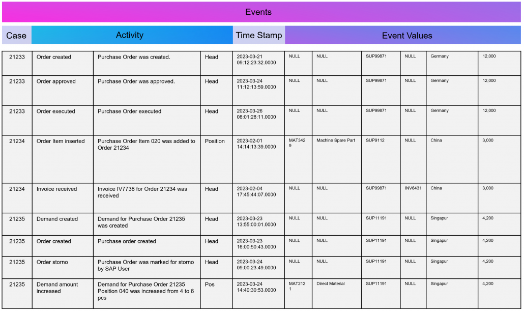
As part of data engineering, the data traces that indicate process activities are brought into a log-like schema. A simple event log is therefore a simple table with the minimum requirement of a process number (case ID), a time stamp and an activity description.

Event Log in Process Mining

Example Event Log for Process Mining

An Event Log can be seen as one big data table containing all the process information. Splitting this big table into several data tables is due to the goal of increasing the efficiency of storing the data in a normalized database.

The following example SQL-query is inserting Event-Activities from a SAP ERP System into an existing event log database table (one big table). It shows that events are based on timestamps (CPUDT, CPUTM) and refer each to one of a list of possible activities (dependent on VGABE).

Attention: Please see this SQL as a pure example of event mining for a classic (single table) event log! It is based on a German SAP ERP configuration with customized processes.

An Event Log can also include many other columns (attributes) that describe the respective process activity in more detail or the higher-level process context.

Incidentally, Process Mining can also work with more than just one timestamp per activity. Even the small Process Mining tool Fluxicon Disco made it possible to handle two activities from the outset. For example, when creating an order in the ERP system, the opening and closing of an input screen could be recorded as a timestamp and the execution time of the micro-task analyzed. This concept is continued as so-called task mining.

Task Mining

Task Mining is a subtype of Process Mining and can utilize user interaction data, which includes keystrokes, mouse clicks or data input on a computer. It can also include user recordings and screenshots with different timestamp intervals.

As Task Mining provides a clearer insight into specific sub-processes, program managers and HR managers can also understand which parts of the process can be automated through tools such as RPA. So whenever you hear that Process Mining can prepare RPA definitions you can expect that Task Mining is the real deal.

Machine Learning for Process and Task Mining on Text and Video Data

Process Mining and Task Mining is already benefiting a lot from Text Recognition (Named-Entity Recognition, NER) by Natural Lamguage Processing (NLP) by identifying events of processes e.g. in text of tickets or e-mails. And even more Task Mining will benefit form Computer Vision since videos of manufacturing processes or traffic situations can be read out. Even MTM analysis can be done with Computer Vision which detects movement and actions in video material.

Object-Centric Process Mining

Object-centric Process Data Modeling is an advanced approach of dynamic data modelling for analyzing complex business processes, especially those involving multiple interconnected entities. Unlike classical process mining, which focuses on linear sequences of activities of a specific process chain, object-centric process mining delves into the intricacies of how different entities, such as orders, items, and invoices, interact with each other. This method is particularly effective in capturing the complexities and many-to-many relationships inherent in modern business processes.

Note from the author: The concept and name of object-centric process mining was introduced by Wil M.P. van der Aalst 2019 and as a product feature term by Celonis in 2022 and is used extensively in marketing. This concept is based on dynamic data modelling. I probably developed my first event log made of dynamic data models back in 2016 and used it for an industrial customer. At that time, I couldn’t use the Celonis tool for this because you could only model very dedicated event logs for Celonis and the tool couldn’t remap the attributes of the event log while on the other hand a tool like Fluxicon disco could easily handle all kinds of attributes in an event log and allowed switching the event perspective e.g. from sales order number to material number or production order number easily.

An object-centric data model is a big deal because it offers the opportunity for a holistic approach and as a database a single source of truth for Process Mining but also for other types of analytical applications.

Enhancement of the Data Model for Obect-Centricity

The Event Log is a data model that stores events and their related attributes. A classic Event Log has next to the Case ID, the timestamp and a activity description also process related attributes containing information e.g. about material, department, user, amounts, units, prices, currencies, volume, volume classes and much much more. This is something we can literally objectify!

The problem of this classic event log approach is that this information is transformed and joined to the Event Log specific to the process it is designed for.

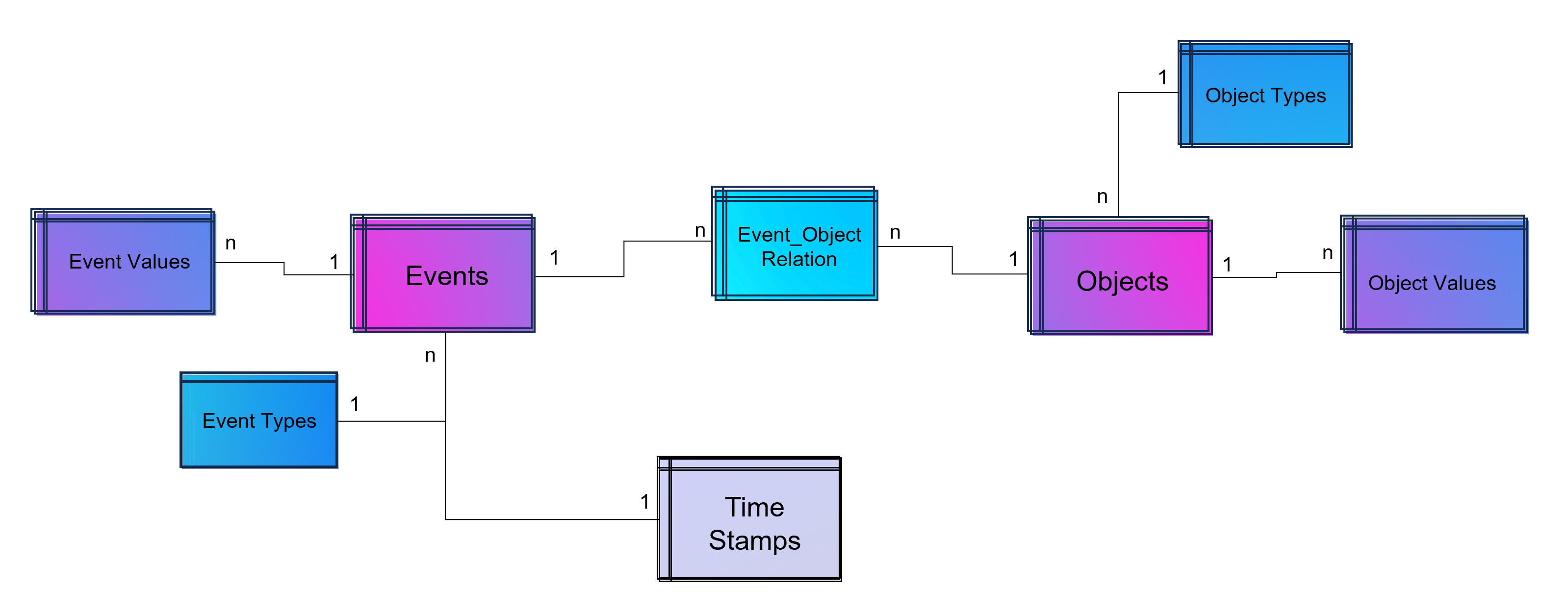
An object-centric event log is a central data store for all kind of events mapped to all relevant objects to these events. For that reason our event log – that brings object into the center of gravity – we need a relational bridge table (Event_Object_Relation) into the focus. This tables creates the n to m relation between events (with their timestamps and other event-specific values) and all objects.

For fulfillment of relational database normalization the object table contains the object attributes only but relates their object attribut values from another table to these objects.

Advanced Event Log with dynamic Relations between Objects and Events

Advanced Event Log with dynamic Relations between Objects and Events

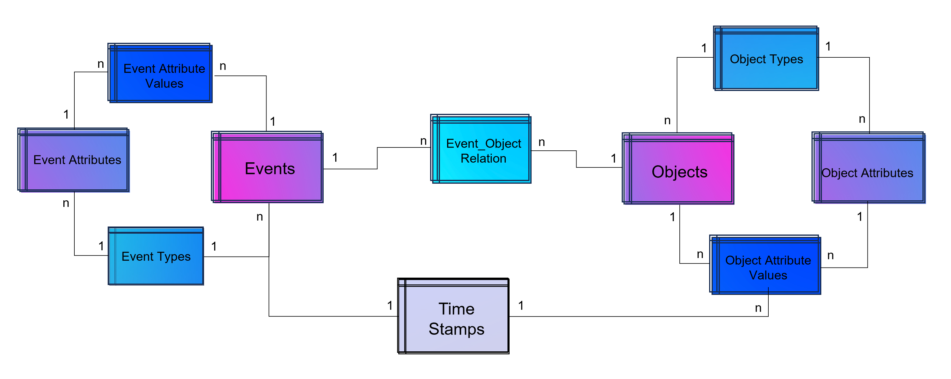
The above showed data model is already object-centric but still can become more dynamic in order to object attributes by object type (e.g. the type material will have different attributes then the type invoice or department). Furthermore the problem that not just events and their activities have timestamps but also objects can have specific timestamps (e.g. deadline or resignation dates).

Advanced Event Log with dynamic Relations between Objects and Events and dynamic bounded attributes and their values to Events - And the same for Objects.

Advanced Event Log with dynamic Relations between Objects and Events and dynamic bounded attributes and their values to Events – And the same for Objects.

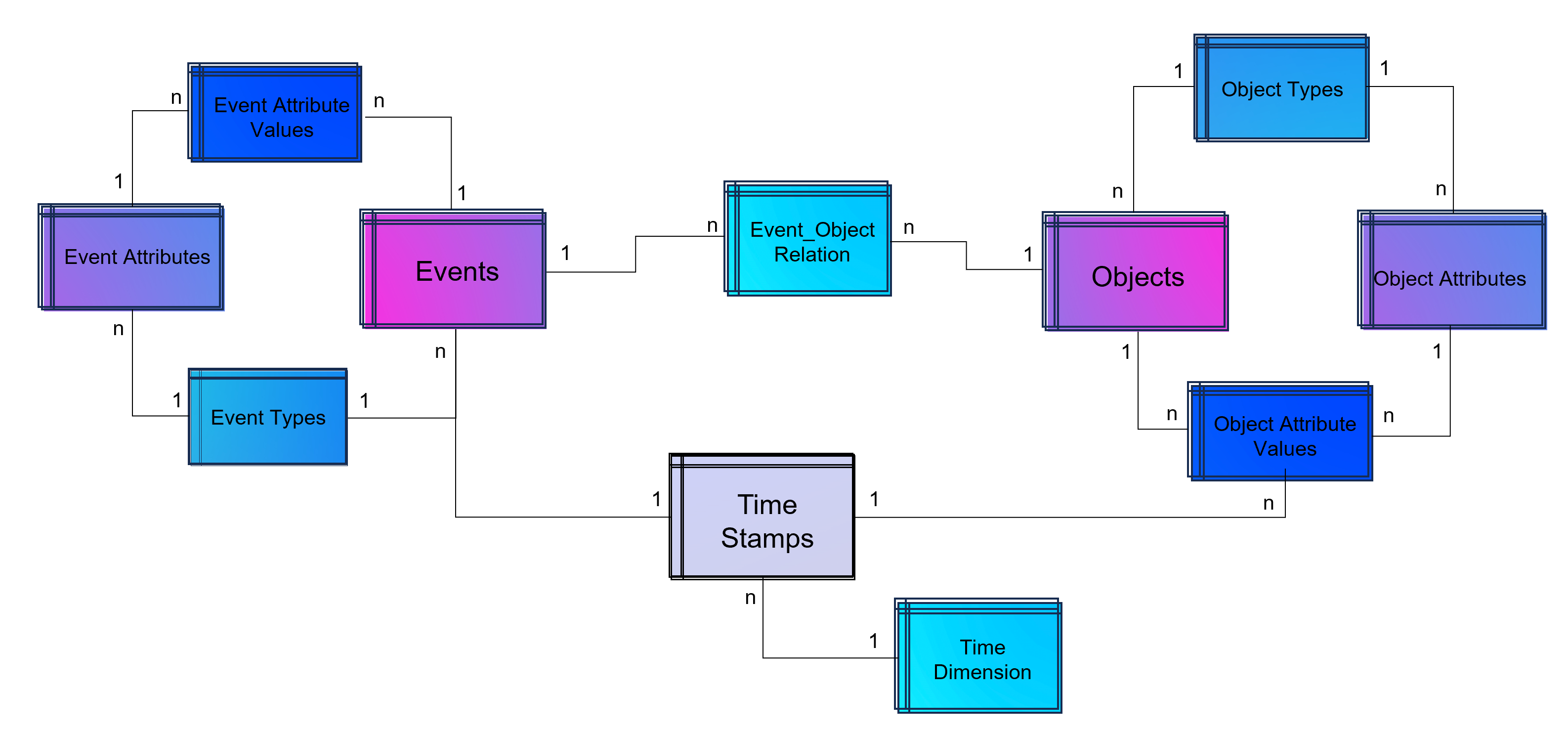
A last step makes the event log data model more easy to analyze with BI tools: Adding a classical time dimension adding information about each timestamp (by date, not by time of day), e.g. weekdays or public holidays.

Advanced Event Log with dynamic Relations between Objects and Events and dynamic bounded attributes and their values to Events and Objects. The measured timestamps (and duration times in case of Task Mining) are enhanced with a time-dimension for BI applications.

Advanced Event Log with dynamic Relations between Objects and Events and dynamic bounded attributes and their values to Events and Objects. The measured timestamps (and duration times in case of Task Mining) are enhanced with a time-dimension for BI applications.

For analysis the way of Business Intelligence this normalized data model can already be used. On the other hand it is also possible to transform it into a fact-dimensional data model like the star schema (Kimball approach). Also Data Science related use cases will find granular data e.g. for training a regression model for predicting duration times by process.

Note from the author: Process Mining is often regarded as a separate discipline of analysis and this is a justified classification, as process mining is essentially a graph analysis based on the event log. Nevertheless, process mining can be considered a sub-discipline of business intelligence. It is therefore hardly surprising that some process mining tools are actually just a plugin for Power BI, Tableau or Qlik.

Storing the Object-Centrc Analytical Data Model on Data Mesh Architecture

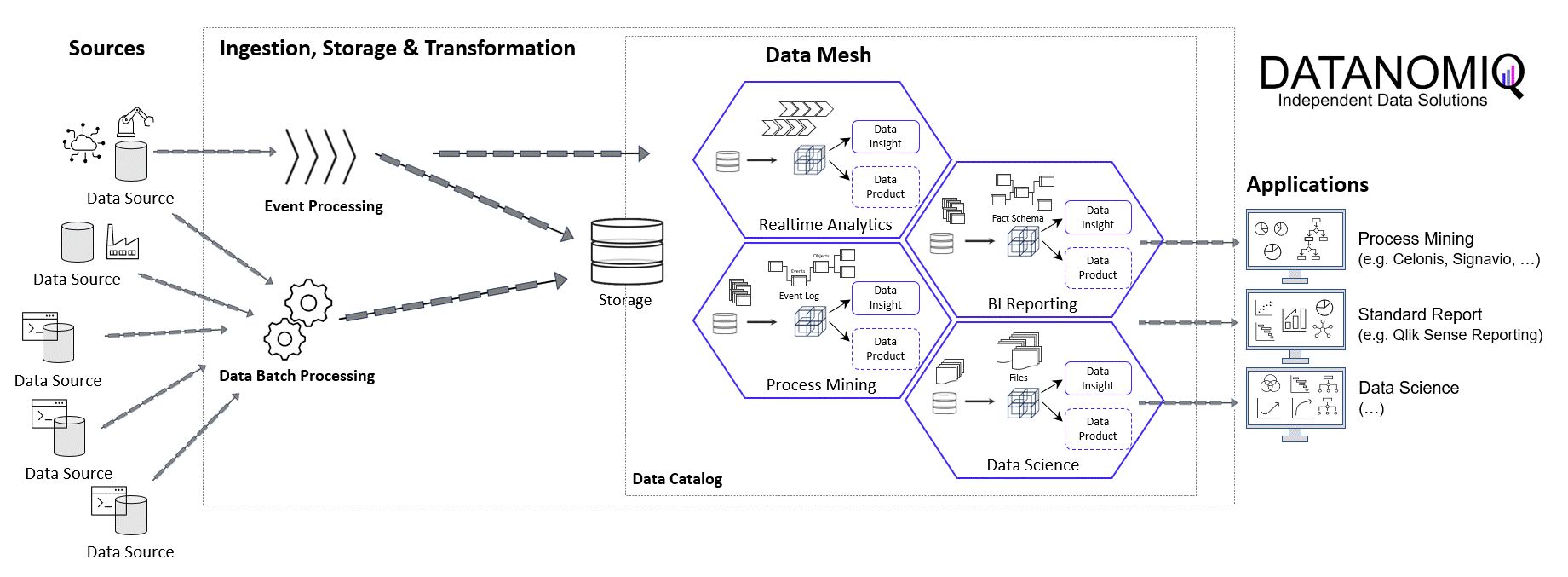
Central data models, particularly when used in a Data Mesh in the Enterprise Cloud, are highly beneficial for Process Mining, Business Intelligence, Data Science, and AI Training. They offer consistency and standardization across data structures, improving data accuracy and integrity. This centralized approach streamlines data governance and management, enhancing efficiency. The scalability and flexibility provided by data mesh architectures on the cloud are very beneficial for handling large datasets useful for all analytical applications.

Note from the author: Process Mining data models are very similar to normalized data models for BI reporting according to Bill Inmon (as a counterpart to Ralph Kimball), but are much more granular. While classic BI is satisfied with the header and item data of orders, process mining also requires all changes to these orders. Process mining therefore exceeds this data requirement. Furthermore, process mining is complementary to data science, for example the prediction of process runtimes or failures. It is therefore all the more important that these efforts in this treasure trove of data are centrally available to the company.

Central single source of truth models also foster collaboration, providing a common data language for cross-functional teams and reducing redundancy, leading to cost savings. They enable quicker data processing and decision-making, support advanced analytics and AI with standardized data formats, and are adaptable to changing business needs.

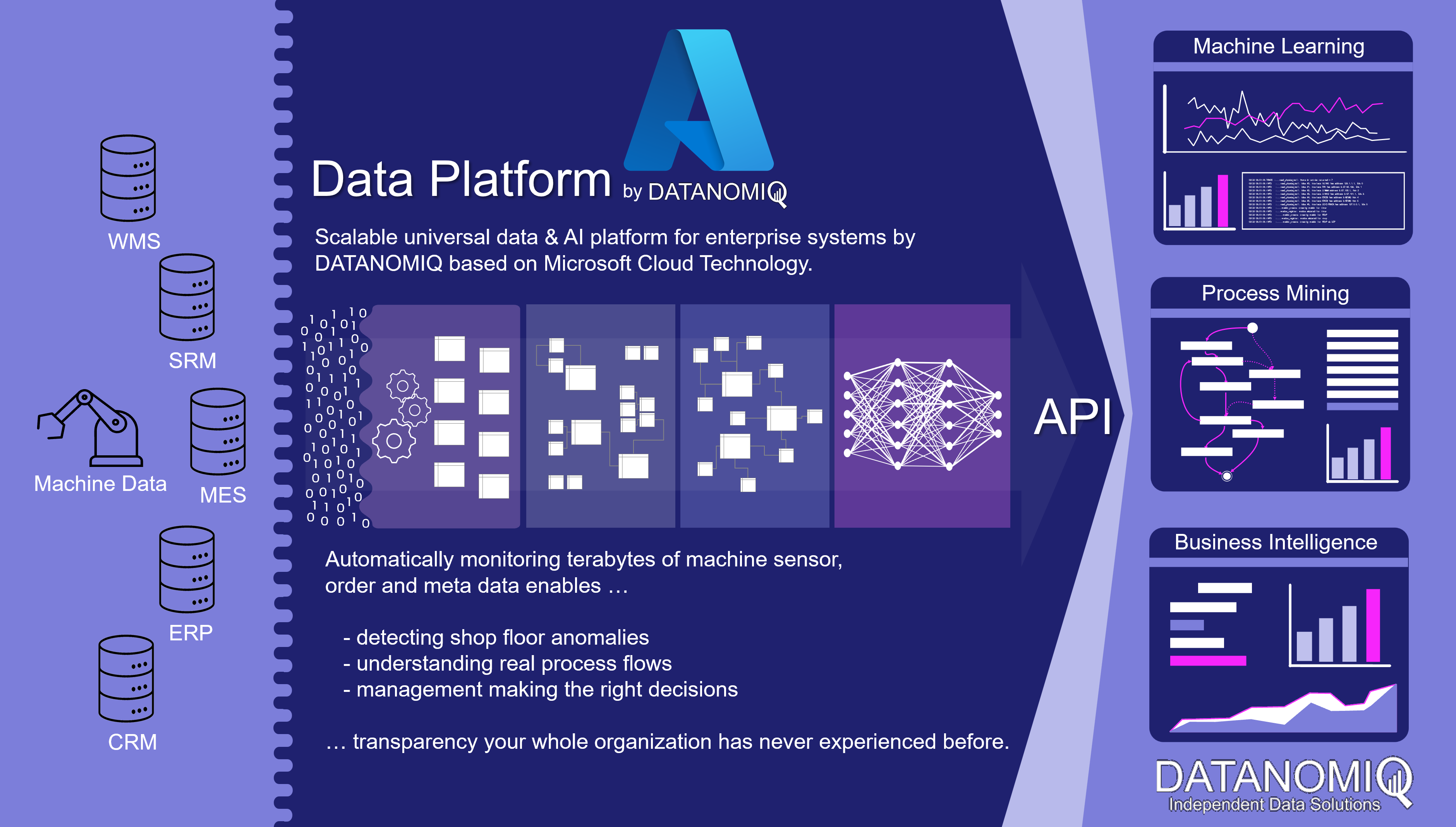
DATANOMIQ Data Mesh Cloud Architecture - This image is animated! Click to enlarge!

DATANOMIQ Data Mesh Cloud Architecture – This image is animated! Click to enlarge!


Central data models in a cloud-based Data Mesh Architecture (e.g. on Microsoft Azure, AWS, Google Cloud Platform or SAP Dataverse) significantly improve data utilization and drive effective business outcomes. And that´s why you should host any object-centric data model not in a dedicated tool for analysis but centralized on a Data Lakehouse System.

About the Process Mining Tool for Object-Centric Process Mining

Celonis is the first tool that can handle object-centric dynamic process mining event logs natively in the event collection. However, it is not neccessary to have Celonis for using object-centric process mining if you have the dynamic data model on your own cloud distributed with the concept of a data mesh. Other tools for process mining such as Signavio, UiPath, and process.science or even the simple desktop tool Fluxicon Disco can be used as well. The important point is that the data mesh approach allows you to easily generate classic event logs for each analysis perspective using the dynamic object-centric data model which can be used for all tools of process visualization…

… and you can also use this central data model to generate data extracts for all other data applications (BI, Data Science, and AI training) as well!

Wie man Web Scraping für den Vertrieb nutzt

Vertrieb in Unternehmen ist wie der Motor, der eine Maschine antreibt. Nur wenn Produkte verkauft werden und neue Kunden sich für ein Unternehmen begeistern, kann der nötige Cashflow generiert werden, der Gebäude, Löhne und alle anderen Kosten rund um das Unternehmen tragen kann.

Wie man diesen Bereich eines Unternehmens mit Data Mining und Web Scraping aktiv unterstützen kann, zeige ich euch in diesem Artikel.

Kernthema im Vertrieb: Leadgenerierung

Jeder Verkauf beginnt mit einer Person, die an unserem Produkt interessiert ist und es kaufen möchte. Ein zentraler Punkt im Vertrieb sind deshalb die “Leads” – Kontaktadresse von Kunden, mit denen wir ins Gespräch kommen können, um ein Angebot zu machen und schließlich unsere Produkte zu verkaufen. Die Leads sind die Basis in jedem Vertriebsprozess, weil wir über diese Daten mit Menschen ins Gespräch kommen können und Beziehungen zu potentiellen Kunden aufbauen können. Je besser diese vorselektiert sind und auf unsere Zielgruppe angepasst sind, desto einfacher wird die Arbeit für unseren Vertrieb.

Leadgenerierung meint dabei das Sammeln von Daten zu Unternehmen oder Personen, die zu unserer Zielgruppe passen und mit möglichst hoher Wahrscheinlichkeit einen Bedarf an unserem Produkt haben. Um in einem Unternehmen einen konstanten Umsatz zu erwirtschaften und die Produktion das ganze Jahr über auszulasten, müssen regelmäßig Aufträge in das Unternehmen kommen. Damit der Vertrieb diese Aufträge an Land ziehen kann, müssen die Vertriebsmitarbeiter immer wieder neue Kundengespräche führen. Und damit diese Gespräche stattfinden können, muss ein Unternehmen auf zuverlässige und wiederholbare Weise immer wieder Leads generieren. Immer wieder neue, potenzielle Interessenten zu finden, ist dabei eine der herausforderndsten Aufgaben jeder Vertriebsleitung.

Leads generieren mit Web Scraping

Mit Web Scraping Leads zu generieren bedeutet Kontaktdaten aus dem Internet zu sammeln mit Hilfe einer Software. Vorwiegend werden dabei Webseiten und frei zugängliche Daten aus allen Ecken des Internets durchsucht mit einem Programm, welches anschließend die Daten in eine übersichtliche Datei, wie beispielsweise Excel, verpackt. Dadurch können diese Daten wiederum sehr einfach in die meisten gängigen CRM (Customer Relationship Management) Systeme hochgeladen werden, wo die Vertriebsteams diese direkt bearbeiten können. Mit dieser Methode lassen sich in kurzer Zeit auf die Zielgruppe spezialisierte Listen erstellen, die dem Unternehmen helfen, neue Kundenkontakte zu finden und zu erstellen.

Die Daten dabei können Namen von Personen oder Unternehmen sein, Adressen, Telefonnummern, E-Mail-Adressen, URLs und mehr. Unternehmen und Start-ups ersparen sich damit die mühsame Arbeit dutzende Webseiten und Datenbanken nach möglichen Kontaktadressen zu suchen. Web Scraper sind dabei auch um einiges effizienter als ein manueller Suchvorgang, weil die Programme oft mit komplexen Algorithmen arbeiten, die immer wieder optimiert werden, um bestmögliche Ergebnisse zu erreichen.

Die Vorteile von Web Scraping zur Leadgenerierung

Durch die Automatisierung eines sonst sehr zeitaufwendigen Prozesses werden die Ressourcen im Unternehmen besser eingesetzt. Vor allem Vertriebsmitarbeiter können sich dadurch besser ihrer eigentlichen Aufgabe widmen: Zeit mit Kunden verbringen.

Viele Mitarbeiter im Vertrieb sind auch spezialisiert auf den Umgang mit Menschen und sind möglicherweise etwas unbeholfen, wenn es darum geht, Daten zu sammeln und dabei Tage nur vor dem Bildschirm zu verbringen. Mit Web Scraping wird diese eintönige Tätigkeit aus dem Alltag dieser Mitarbeiter herausgenommen. Die Mitarbeiter können den Tätigkeiten auf die sie spezialisiert sind mehr Zeit widmen, und es müssen auch keine teuren Mitarbeiter mehr abgestellt werden für eine Tätigkeit, die ohnehin maschinell besser gelöst werden kann.

Durch die Analyse von unzähligen Daten beim Web Scraping lassen sich manchmal auch bereits Hypothesen über unsere Zielgruppe überprüfen. Dadurch lernen wir bereits vorab, wie unsere Kunden arbeiten, was für sie relevante Themen sind und wie wir sie am besten ansprechen können. Mit Hilfe dieser Daten können wir wiederum bessere Entscheidungen im Marketing und Vertrieb treffen, basierend auf dem echten Verhalten unserer Kunden anstatt nur auf Vermutungen.

Mit Hilfe der Kombination aus effizientem Ressourceneinsatz sowohl von personeller, zeitlicher als auch monetärer Perspektive und die gleichzeitige Auswertung von Daten über Kunden und deren Verhalten lassen sich langfristige Vorteile für ein Unternehmen erzeugen mit denen man der Konkurrenz einen Schritt voraus ist. Richtig umgesetzt lassen sich damit Geschäftsmöglichkeiten und Umsatzpotenziale lukrieren, noch bevor diese am Markt öffentlich bekannt werden.

Die Herausforderungen beim Web Scraping

Wenn diese Taktik so umwerfend funktioniert, warum macht es dann nicht jeder?

Natürlich gibt es auch beim Web Scraping einige Herausforderungen, die zu beachten sind.

Das offensichtlichste davon ist die Qualität der Daten. Auch das komplexeste Programm kann nur die Daten aus dem Internet filtern, die dort öffentlich zugänglich sind. Dies bedeutet aber auch, dass manches davon nicht mehr aktuell ist, anderes wird irrelevant sein und ein Teil davon als Leads für den Vertrieb gar nicht zu gebrauchen.

Dazu kommen Restriktionen beim Crawlen von Webseiten. Viele Seiten blockieren bewusst Crawler und sind sehr sensibel beim Umgang mit deren Daten, was erneut zu Problemen führen kann. In vielen Fällen müssen diese Seiten ausgeschlossen werden oder sind gar nicht für die Leadgenerierung zu gebrauchen. CAPTCHAs sind dabei nur eine der möglichen Hürden, die den Prozess entweder stark verlangsamen oder völlig stoppen können.

Doch auch selbst wenn Daten frei zugänglich zu finden sind, kommen diese oft mehr als ein Mal vor auf diversen Quellen im Netz. Dies sorgt in den Ergebnissen der Scraper oft für Duplikate. Dabei kann auch der Aufbau einer Webseite Schwierigkeiten bereiten, zumal diese unterschiedlich strukturiert und angeordnet sein können, wodurch eine einheitliche Programmierung für das Scraping schwer zu gestalten ist. Hinzu kommen noch technologische Barrieren, die im Netz verbaut sein können, wie die Nutzung von Javascript, dynamischer Content, oder andere Hindernisse auf den verschiedenen Webseiten.

Geeignete Webseiten oder Plattformen finden

Bevor man mit dem Scraping starten kann, muss man zuerst festlegen, welche Seiten oder Plattformen man überhaupt durchsuchen will. Hier sind einige der Faktoren, die man dabei beachten sollte:

Wo finde ich meine Zielgruppe?

Am besten beginnen wir unsere Suche dort, wo unsere Kunden ohnehin bereits sind, wo sie ihre Freizeit verbringen oder nach Informationen suchen. In B2B Märkten können wir alternativ immer die eigenen Webseiten unserer Kunden durchsuchen.

Wie relevant ist die Seite für mein Produkt?

Es ergibt keinen Sinn Seiten zu crawlen, die nichts mit unseren Produkten zu tun haben und bei denen die Nutzer auch nichts mit unserem Produkt anfangen können. Wer beispielsweise Haarpflegeprodukte verkauft, sollte kein Bauforum durchsuchen.

Wie aktuell ist die Webseite?

Wer Daten auf veralteten Webseiten sucht, wird auch nur veraltete Daten finden. Diese sind meistens kaum bis gar nicht brauchbar für den Vertrieb. Die angegebenen Seiten sollten daher möglichst aktuell sein und die Daten darauf regelmäßig aktualisiert werden.

Rechtliche Abklärung

Manche Seiten verbieten explizit das Benutzen jeglicher Daten zu kommerziellen Zwecken. Dies sollte genau analysiert werden, bevor man Daten von einer Seite extrahiert.

Verfügbarkeit und Qualität der Daten:

Manche Seiten machen es Crawlern bewusst schwer an Daten zu kommen, bei manchen bekommt man keinerlei Informationen mehr ohne Captcha Überprüfung, Opt-In Formular, etc. Auch ein Aufbau der Seite in komplexem HTML Code oder Ähnliches kann Scraping zu einer Herausforderung werden lassen, die einem viel Zeit kostet, anstatt sie zu gewinnen.

Beispiele für Web Scraping

Genug mit der Theorie, sehen wir uns nun ein paar konkrete Beispiele an. Im Idealfall hat man einen Programmierer im Unternehmen zur Verfügung, der gerade keine anderen Projekte verfolgen muss und genug Zeit hat, um einen eigenen Web Scraper zu bauen, zielgerichtet auf die Bedürfnisse des Unternehmens. Dieser kann genau auf die Produkte, rechtlichen Anforderungen und die optimalen Kunden für den Vertrieb programmiert werden. Realistisch gesehen, kommt dieses Szenario nur äußerst selten vor. Deshalb stellen wir euch hier einige vorgefertigte Lösungen vor. Die richtige Lösung wird sich bei jedem Unternehmen nach Produkten, Marktlage, Kundenverhalten etc. unterscheiden und muss individuell an jedes Unternehmen angepasst sein.

io

Am Beginn des Vertriebsprozesses brauchen wir eine große Anzahl an Leads. Import.io ist genau einer der Anbieter, die dabei helfen können, große Mengen an Daten aus dem Internet zu erzeugen. Wichtig dabei ist, dass unser restlicher Vertriebsprozess soweit fortgeschritten sein muss, dass wir genau unsere Zielgruppe kennen und wissen, wo und wie man diese Personen finden kann.

Das praktische an dieser Plattform ist, dass man absolut nichts coden oder programmieren muss. Übrigens ist Import.io ursprünglich nicht für Vertriebs- und Marketingzwecke entworfen worden, wird aber immer wieder von gewieften Sales Managern und Marketern als Geheimtipp genutzt. Die Technologie eignet sich hervorragend, um große Listen an Leads mit Web Scraping zu erzeugen.

Die Daten können als .csv Datei gesammelt und von dort optimal in das CRM System der Wahl integriert werden.

Scrape-it Marktplatz

Wer Kundendaten vorwiegend über öffentliche Seiten wie Yellow Pages, Booking.com oder Google Maps finden kann, hat hier ein breites Angebot an verschiedenen Scraper zur Auswahl. Alle davon erfordern keinerlei Programmierung und sind bereit zum Einsatz nach dem Download. Wer beispielsweise Architekten in Barcelona oder Restaurants in Paris als Leads nutzen kann, für den bieten diese Lösungen einen schnellen Zugang zu einer Menge an Daten.

Octoparse

Eine weitere Lösung, die ohne jede Programmierung und Vorkenntnis angewendet werden kann, um schnell große Mengen an Leads zu generieren. Dieses Programm hat eine besonders einfach zu bedienende Oberfläche und wurde direkt für die Leadgenerierung entwickelt.

80legs

Ebenfalls ein sehr nützliches Tool zum Web Scraping, mit dem man viele spezifische Einstellungen vornehmen kann. Zusätzlich bietet dieses Tool auch noch die Möglichkeit, die Daten sofort herunterzuladen. Es ist bestens geeignet um eine breite Basis an Leads zu generieren

Webharvy

Eine einfache Point-and-Click Software als Web Scraper, die einen URLs, E-Mail Adressen, Bilder und Texte von Webseiten sammeln kann. Auch dieses Tool lässt sich einfach ohne jede Programmierung intuitiv bedienen

Scraper

Eine Erweiterung für Google Chrome, die zwar nur begrenzte Daten sammeln kann, aber dennoch ein sehr hilfreiches Tool für die Onlinerecherche. Es ist geeignet für Beginner und Profis gleichermaßen, die Daten lassen sich bequem extrahieren und wie bei den anderen Programmen in eine .csv oder Ähnliche Datei verpacken.

com

Als open-source-basierter Cloud-Service für Webscraping handelt es sich hier um einen unabhängigen und hoch effektiven Web Scraper. Dadurch wird das Programm auch stetig upgedatet und verbessert. Die Software verwendet einen intelligenten Proxy Rotator, der darauf spezialisiert ist, die gängigen Maßnahmen gegen Bots auf Webseiten zu umgehen und trotz vorhandener Gegenmaßnahmen verlässlich die Daten zu sammeln. Sollte man Probleme mit dem Tool haben, steht ein zuverlässiges Support Team zur Verfügung, um bei Fragen zu helfen.

Fazit

Wer im Vertrieb arbeitet oder beispielsweise als Unternehmer auf einen starken, zuverlässigen Vertriebsprozess angewiesen ist, für den lässt sich das Thema Data Mining und Web Scraping heute nicht mehr länger ignorieren. Gerade in den noch “konservativen” Branchen, in denen nicht viel mit diesen digitalen Tools gearbeitet wird, lässt sich durch gekonnten Einsatz von Technologie ein Wettbewerbsvorteil erzeugen. Die Unternehmen, die gewillt sind sich auf diese neue Technologie einzulassen, können damit schneller und gezielter neue Kunden ansprechen und deren Produkte um ein Vielfaches effektiver vermarkten als jene Konkurrenten, die diese Tools nicht einsetzen.

Monitoring of Jobskills with Data Engineering & AI

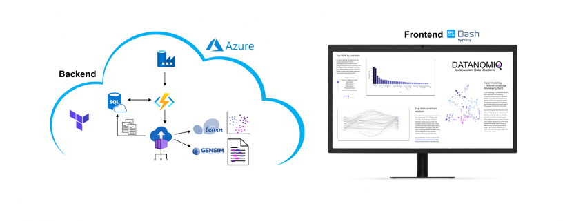
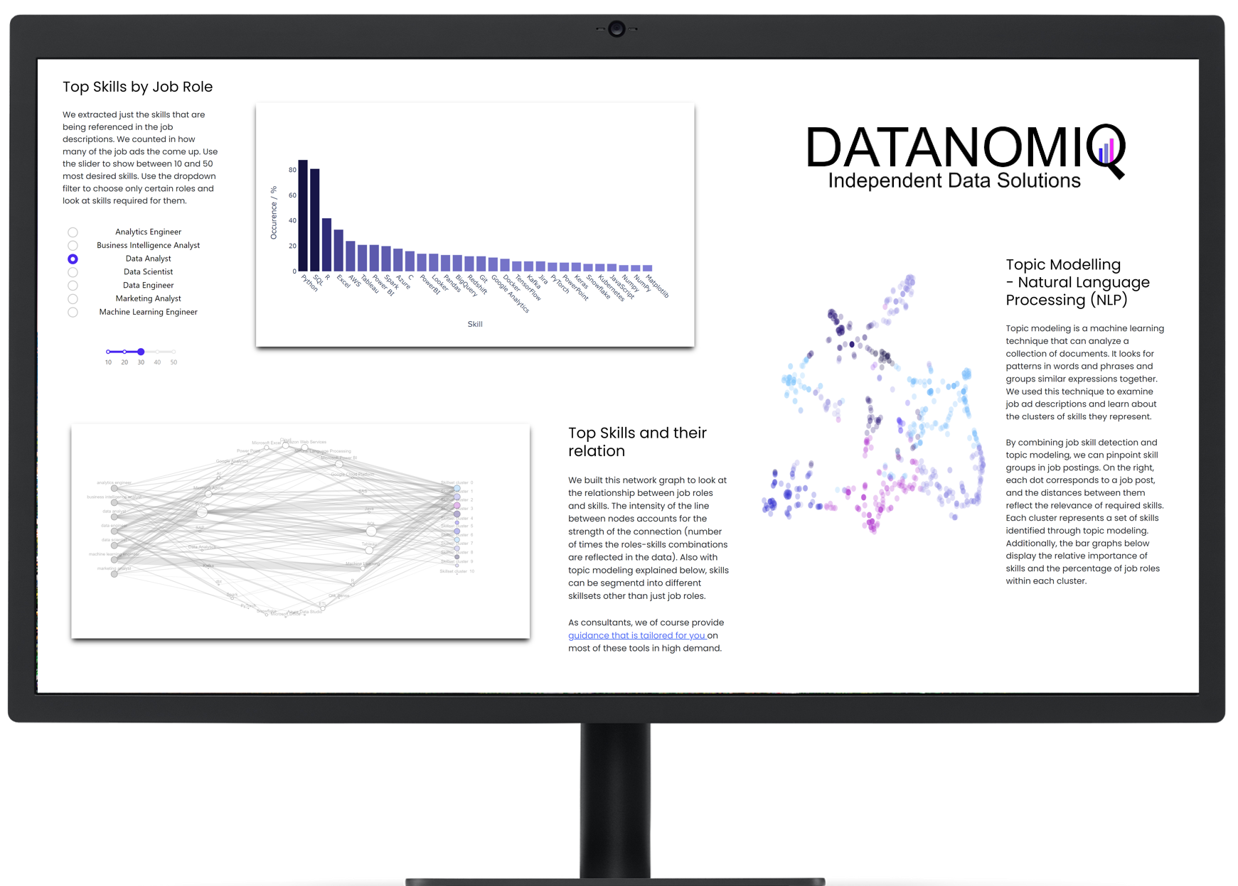
On own account, we from DATANOMIQ have created a web application that monitors data about job postings related to Data & AI from multiple sources (Indeed.com, Google Jobs, Stepstone.de and more).

The data is obtained from the Internet via APIs and web scraping, and the job titles and the skills listed in them are identified and extracted from them using Natural Language Processing (NLP) or more specific from Named-Entity Recognition (NER).

The skill clusters are formed via the discipline of Topic Modelling, a method from unsupervised machine learning, which show the differences in the distribution of requirements between them.

The whole web app is hosted and deployed on the Microsoft Azure Cloud via CI/CD and Infrastructure as Code (IaC).

The presentation is currently limited to the current situation on the labor market. However, we collect these over time and will make trends secure, for example how the demand for Python, SQL or specific tools such as dbt or Power BI changes.

Why we did it? It is a nice show-case many people are interested in. Over the time, it will provides you the answer on your questions related to which tool to learn! For DATANOMIQ this is a show-case of the coming Data as a Service (DaaS) Business.

How to reduce costs for Process Mining

Process mining has emerged as a powerful Business Process Intelligence discipline (BPI) for analyzing and improving business processes. It involves extracting data from source systems to gain insights into process behavior and uncover opportunities for optimization. While there are many approaches to create value with process mining, organizations often face challenges when it comes to the cost of implementing the necessary solution. In this article, we will highlight the key elements when it comes to process mining architectures as well as the most common mistakes, to help organizations leverage the power of process mining while maintain cost control.

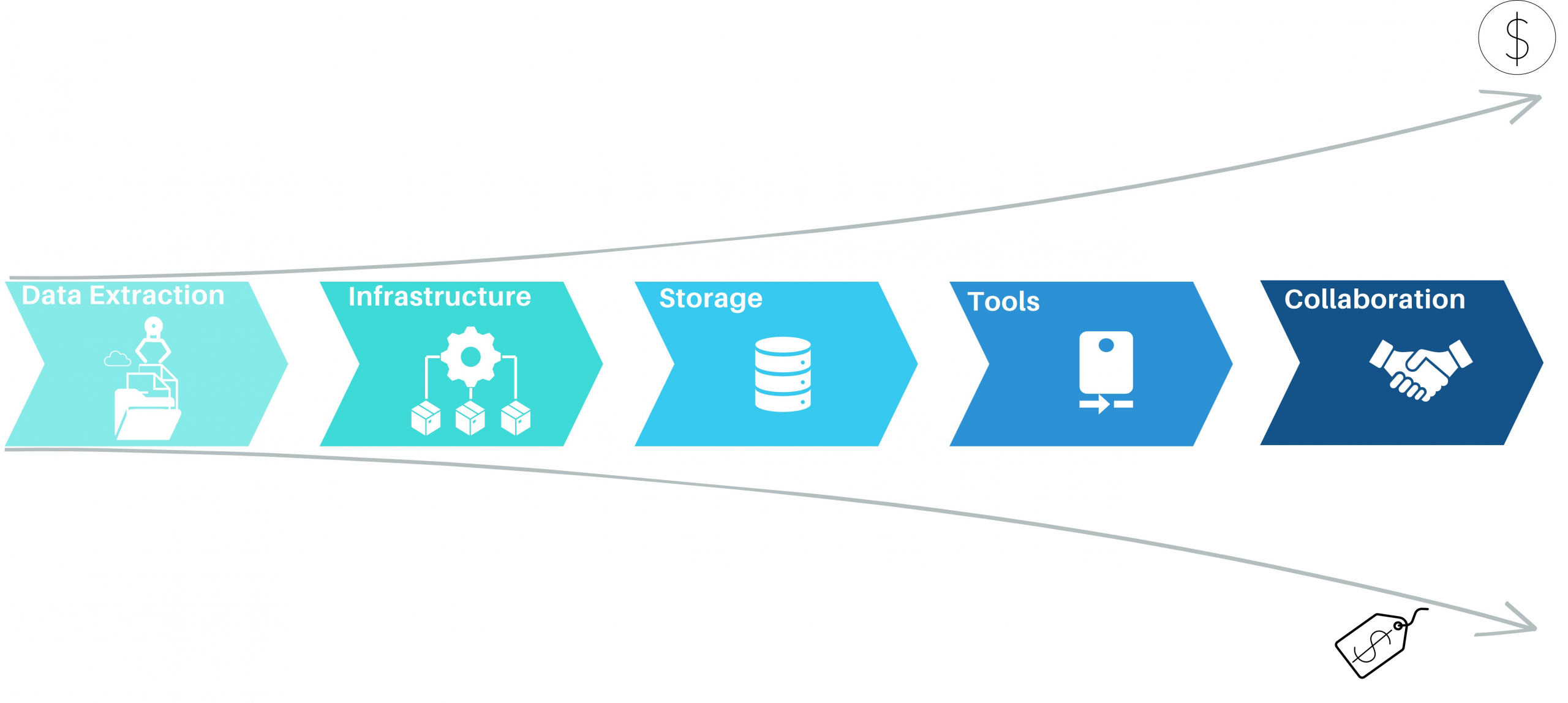
Process Mining - Elements of Process Mining and their cost aspects

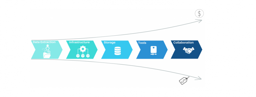
Process Mining – Elements of Process Mining and their cost aspects

Data Extraction for process mining

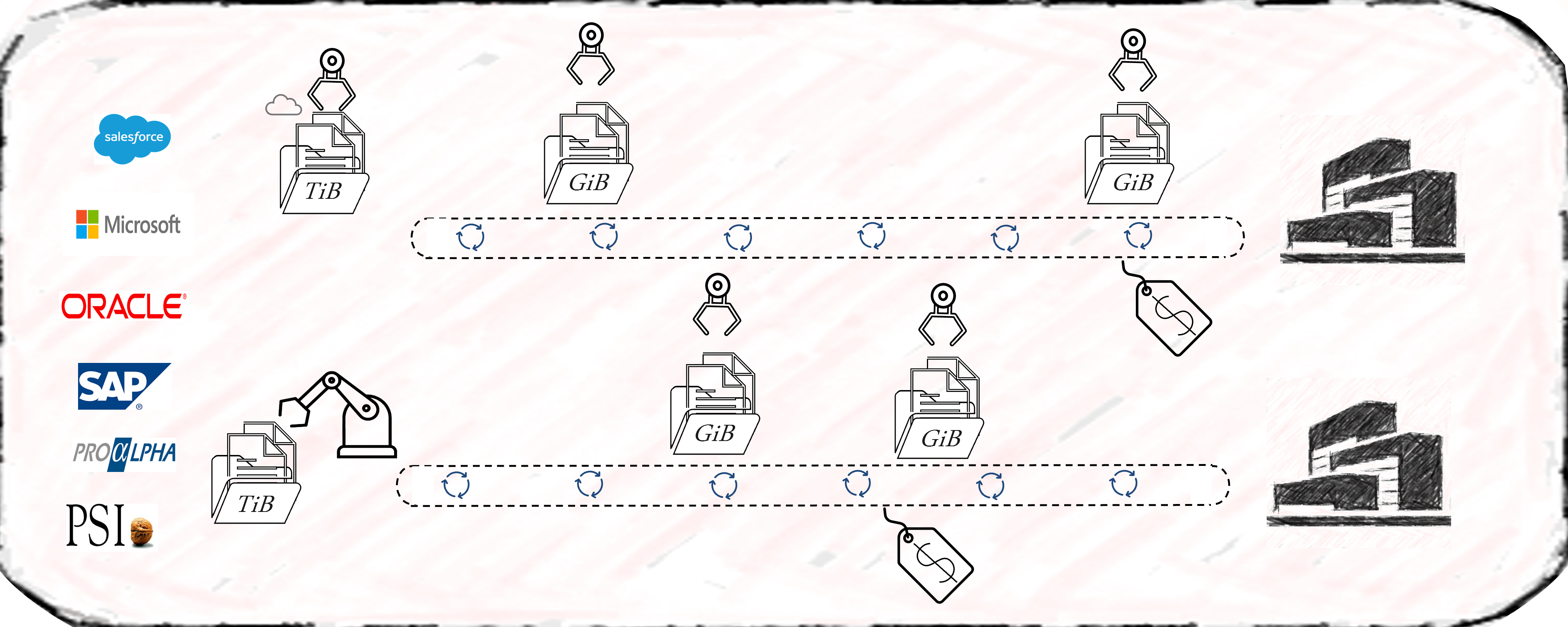
Most process mining projects underestimate the complexity of data extraction. Even for well-known sources like SAP-ERP’s, the extraction often consumes 50% of the first pilot’s resources. As a result, the extraction pipelines are often built with the credo of “asap” and this is where the cost-drama begins. Process Mining demands Big Data in 99% of the cases, releasing bad developed extraction jobs will end in big cost chunks down the value stream. Frequently organizations perform full loads of big SAP tables, causing source system performance impact, increasing maintenance, and moving hundred GB’s of data on daily basis without any new value. Other organizations fall for the connectors, provided by some process mining platform tools, promising time-to-value being the best. Against all odds the data is getting extracted then into costly third-party platforms where they can be only consumed by the platforms process mining tool itself. On top of that, these organizations often perform more than one Business Process Intelligence discipline, resulting in extracting the exact same data multiple times.

Process Mining - Data Extraction

Process Mining – Data Extraction

The data extraction for process mining should be well planed and match the data strategy of the organization. By considering lightweighted data preprocessing techniques organizations can save both time and money. When accepting the investment character of big data extractions, the investment should be done properly in the beginning and therefore cost beneficial in the long term.

Cloud-Based infrastructure with process mining?

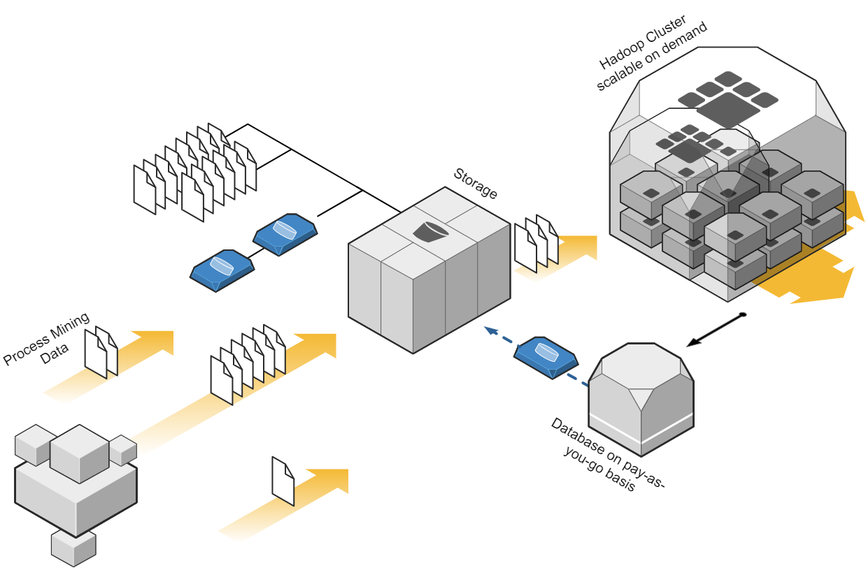
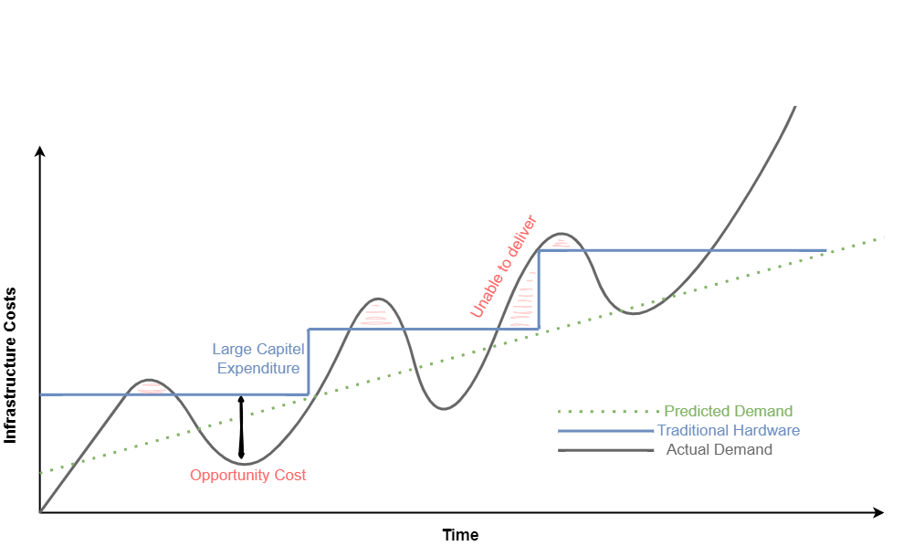
Depending on the data strategy of one organization, one cost-effective approach to process mining could be to leverage cloud computing resources. Cloud platforms, such as Amazon Web Services (AWS), Microsoft Azure, or Google Cloud Platform (GCP), provide scalable and flexible infrastructure options. By using cloud services, organizations can avoid the upfront investment in hardware and maintenance costs associated with on-premises infrastructure. They can pay for resources on a pay-as-you-go basis, scaling up or down as needed, which can significantly reduce costs. When dealing with big data in the cloud, meeting the performance requirements while keeping cost control can be a balancing act, that requires a high skillset in cloud technologies. Depending the organization situation and data strategy, on premises or hybrid approaches should be also considered. But costs won’t decrease only migrating from on-premises to cloud and vice versa. What makes the difference is a smart ETL design capturing the nature of process mining data.

Process Mining Cloud Architecture on "pay as you go" base.

Process Mining Cloud Architecture on “pay as you go” base.

Storage for process mining data

Storing data is a crucial aspect of process mining, as in most cases big data is involved. Instead of investing in expensive data storage solutions, which some process mining solutions offer, organizations can opt for cost-effective alternatives. Cloud storage services like Amazon S3, Azure Blob Storage, or Google Cloud Storage provide highly scalable and durable storage options at a fraction of the cost of process mining storage systems. By utilizing these services, organizations can store large volumes of event data without incurring substantial expenses. Moreover, when big data engineering technics, consider profound process mining logics the storage cost cut down can be tremendous.

Process Mining - Infrastructure Cost Curve - On-Premise vs Cloud

Process Mining – Infrastructure Cost Curve: On-Premise vs Cloud

Process Mining Tools

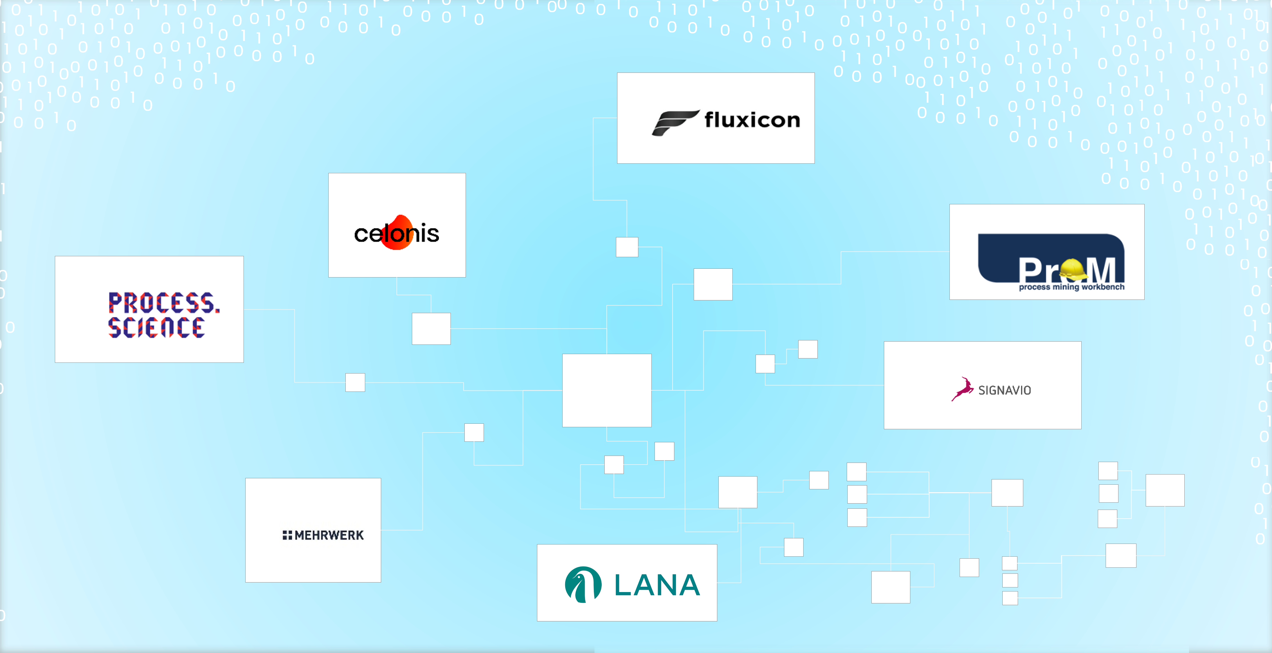
While some commercial process mining tools can be expensive, there are several powerful more economical alternatives available. Tools like Process Science, ProM, and Disco provide comprehensive process mining capabilities without the hefty price tag. These tools offer functionalities such as event log import, process discovery, conformance checking, and performance analysis. Organizations often mismanage the fact, that there can and should be more then one process mining tool available. As expensive solutions like Celonis have their benefits, not all use cases make up for the price of these tools. As a result, these low ROI-use cases will eat up the margin, or (and that’s even more critical) little promising use cases won’t be investigated on and therefore high hanging fruits never discovered. Leveraging process mining tools can significantly reduce costs while still enabling organizations to achieve valuable process insights.

Process Mining Tool Landscape

Process Mining Tool Landscape (examples shown)

Collaboration

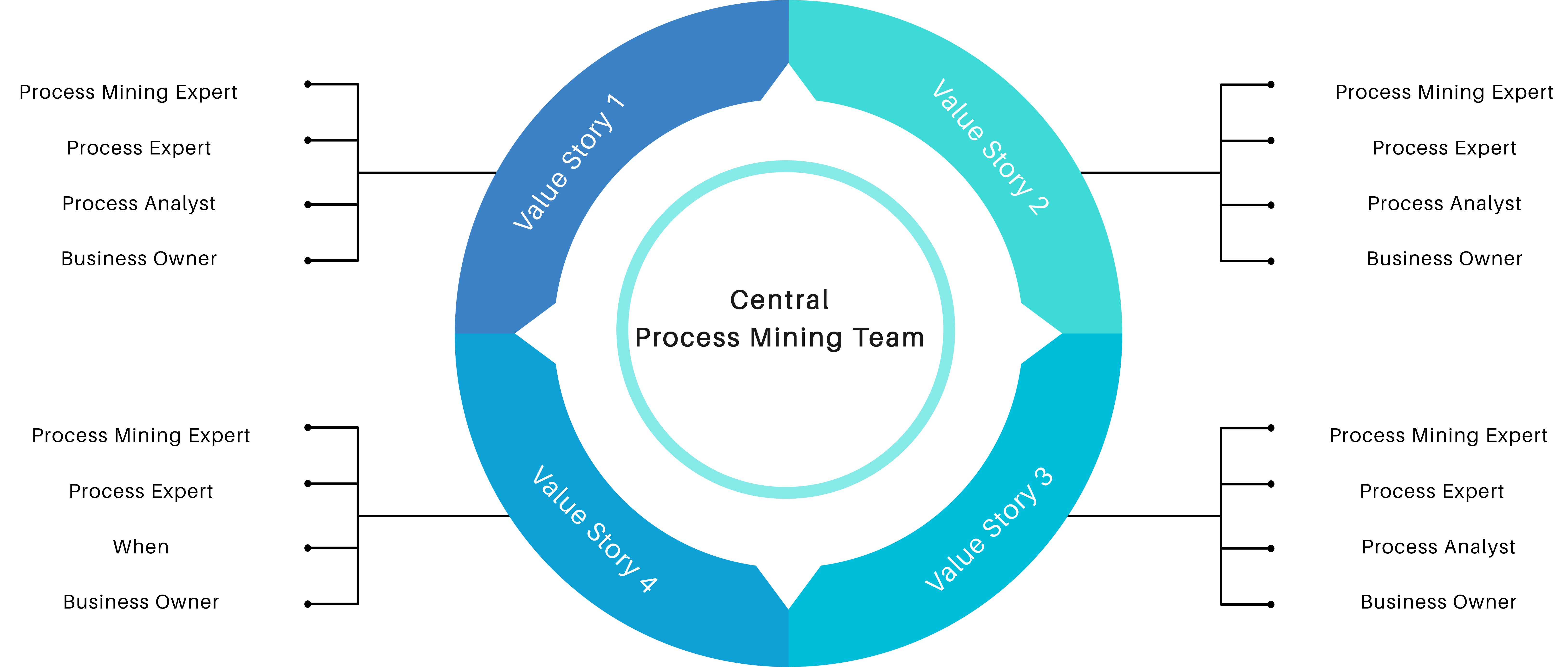
Another cost-saving aspect is to encourage collaboration within the organization itself. Most process mining initiatives require the input from process experts and often involve multiple stakeholders across different departments. By establishing cross-functional teams and supporting collaboration, organizations can share resources and distribute the cost burden. This approach allows for the pooling of expertise, reduces duplication of efforts, and facilitates knowledge exchange, all while keeping costs low.

Process Mining Team Structure

Process Mining Team Structure

Conclusion

Process mining offers tremendous potential for organizations seeking to optimize their business processes. While many organizations start process mining projects euphorically, the costs set an abrupt end to the party. Implementing a low-cost and collaborative architecture can help to create a sustainable value for the organization. By leveraging cloud-based infrastructure, cost-effective storage solutions, big data engineering techniques, process mining tools, well developed data extractions, lightweight data preprocessing techniques, and fostering collaboration, organizations can embark on process mining initiatives without straining their budgets. With the right approach, organizations can unlock the power of process mining and drive operational excellence without losing cost control.

One might argue that implementing process mining is not only about the costs. In the end each organization must consider the long-term benefits and return on investment (ROI). But with a cost controlled and sustainable process mining approach, return on investment is likely higher and less risky.

This article provides general information for process mining cost reduction. Specific strategic decisions should always consider the unique requirements and restrictions of individual organizations.

Was ist eine Vektor-Datenbank? Und warum spielt sie für AI eine so große Rolle?

Wie können Unternehmen und andere Organisationen sicherstellen, dass kein Wissen verloren geht? Intranet, ERP, CRM, DMS oder letztendlich einfach Datenbanken mögen die erste Antwort darauf sein. Doch Datenbanken sind nicht gleich Datenbanken, ganz besonders, da operative IT-Systeme meistens auf relationalen Datenbanken aufsetzen. In diesen geht nur leider dann doch irgendwann das Wissen verloren… Und das auch dann, wenn es nie aus ihnen herausgelöscht wird!

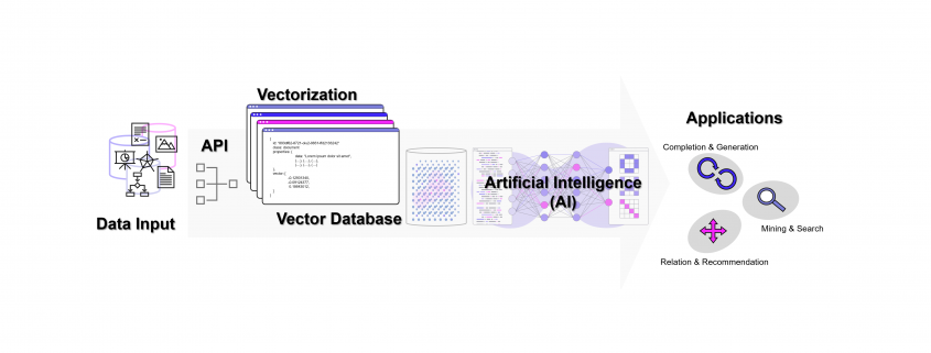
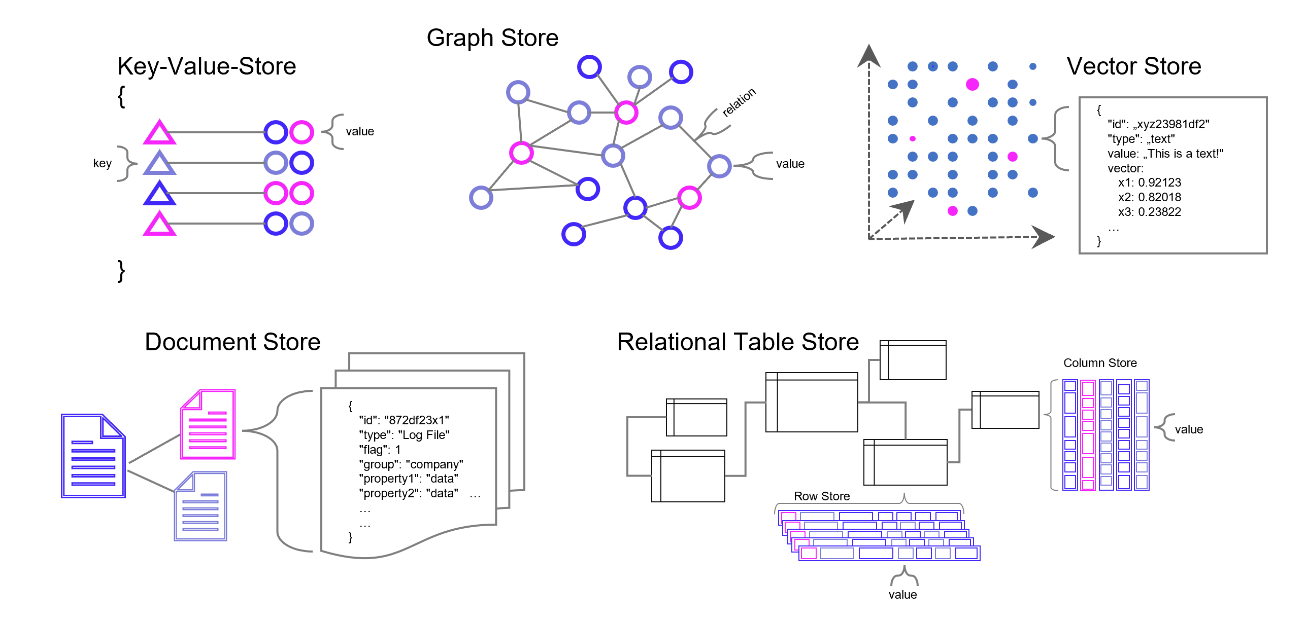
Die meisten Datenbanken sind darauf ausgelegt, Daten zu speichern und wieder abrufbar zu machen. Neben den relationalen Datenbanken (SQL) gibt es auch die NoSQL-Datenbanken wie den Key-Value-Store, Dokumenten- und Graph-Datenbanken mit recht speziellen Anwendungsgebieten. Vektor-Datenbanken sind ein weiterer Typ von Datenbank, die unter Einsatz von AI (Deep Learning, n-grams, …) Wissen in Vektoren übersetzen und damit vergleichbarer und wieder auffindbarer machen. Diese Funktion der Datenbank spielt seinen Vorteil insbesondere bei vielen Dimensionen aus, wie sie Text- und Bild-Daten haben.

Databases Types: Vector Database, Graph Database, Key-Value-Database, Document Database, Relational Database with Row or Column oriented table structures

Datenbank-Typen in grobkörniger Darstellung. Es gibt in der Realität jedoch viele Feinheiten, Übergänge und Überbrückungen zwischen den Datenbanktypen, z. B. zwischen emulierter und nativer Graph-Datenbank. Manche Dokumenten- Vektor-Datenbanken können auch relationale Datenmodellierung. Und eigentlich relationale Datenbanken wie z. B. PostgreSQL können mit Zusatzmodulen auch Vektoren verarbeiten.

Vektor-Datenbanken speichern Daten grundsätzlich nicht relational oder in einer anderen Form menschlich konstruierter Verbindungen. Dennoch sichert die Datenbank gewissermaßen Verbindungen indirekt, die von Menschen jedoch – in einem hochdimensionalen Raum – nicht mehr hergeleitet werden können und sich auf bestimmte Kontexte beziehen, die sich aus den Daten selbst ergeben. Maschinelles Lernen kommt mit der nummerischen Auflösung von Text- und Bild-Daten (und natürlich auch bei ganz anderen Daten, z. B. Sound) am besten zurecht und genau dafür sind Vektor-Datenbanken unschlagbar.

Was ist eine Vektor-Datenbank?

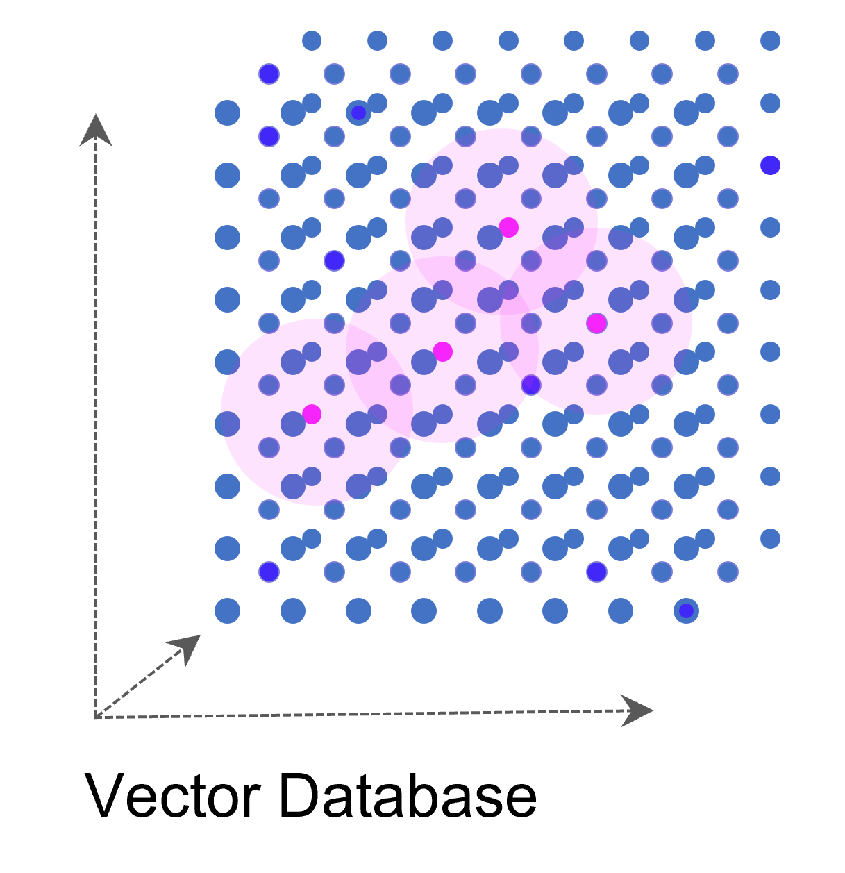
Eine Vektordatenbank speichert Vektoren neben den traditionellen Datenformaten (Annotation) ab. Ein Vektor ist eine mathematische Struktur, ein Element in einem Vektorraum, der eine Reihe von Dimensionen hat (oder zumindest dann interessant wird, genaugenommen starten wir beim Null-Vektor). Jede Dimension in einem Vektor repräsentiert eine Art von Information oder Merkmal. Ein gutes Beispiel ist ein Vektor, der ein Bild repräsentiert: jede Dimension könnte die Intensität eines bestimmten Pixels in dem Bild repräsentieren.
Auf dieseVektor Datenbank Illustration (vereinfacht, symbolisch) Weise kann eine ganze Sammlung von Bildern als eine Sammlung von Vektoren dargestellt werden. Noch gängiger jedoch sind Vektorräume, die Texte z. B. über die Häufigkeit des Auftretens von Textbausteinen (Wörter, Silben, Buchstaben) in sich einbetten (Embeddings). Embeddings sind folglich Vektoren, die durch die Projektion des Textes auf einen Vektorraum entstehen.

Vektor-Datenbanken sind besonders nützlich, wenn man Ähnlichkeiten zwischen Vektoren finden muss, z. B. ähnliche Bilder in einer Sammlung oder die Wörter “Hund” und “Katze”, die zwar in ihren Buchstaben keine Ähnlichkeit haben, jedoch in ihrem Kontext als Haustiere. Mit Vektor-Algorithmen können diese Ähnlichkeiten schnell und effizient aufgespürt werden, was sich mit traditionellen relationalen Datenbanken sehr viel schwieriger und vor allem ineffizienter darstellt.

Vektordatenbanken können auch hochdimensionale Daten effizient verarbeiten, was in vielen modernen Anwendungen, wie zum Beispiel Deep Learning, wichtig ist. Einige Beispiele für Vektordatenbanken sind Elasticsearch / Vector Search, Weaviate, Faiss von Facebook und Annoy von Spotify.

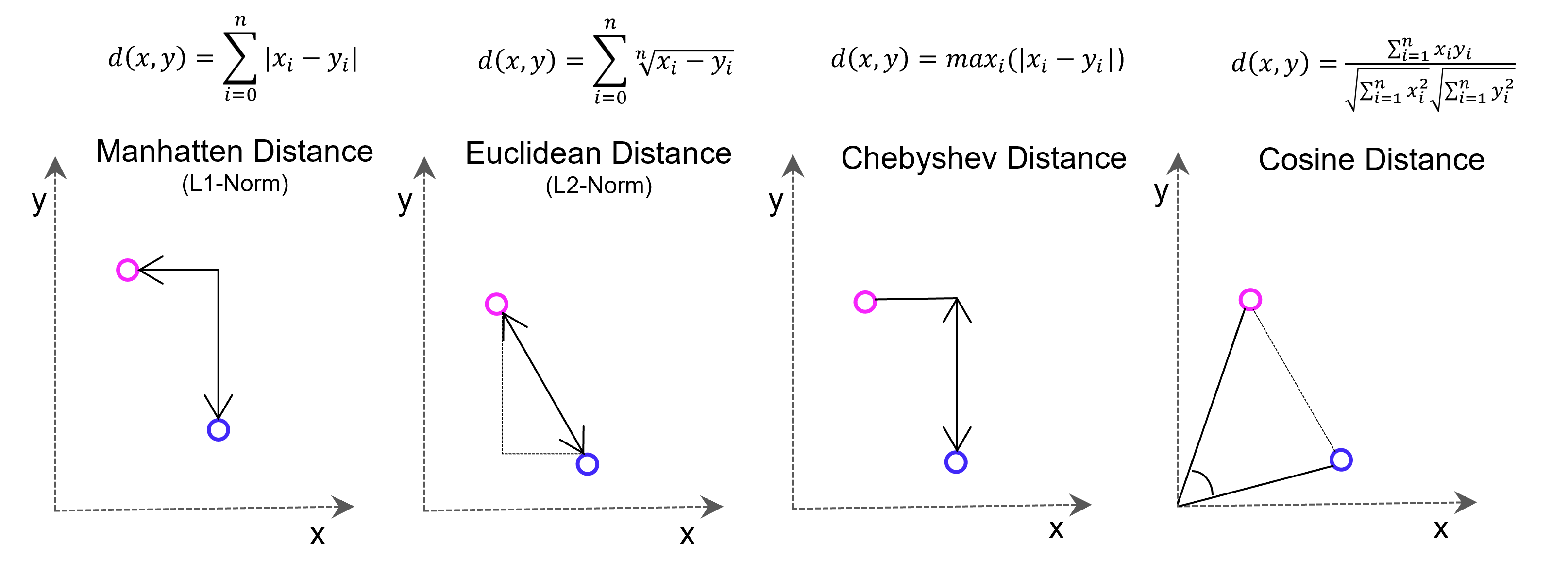
Viele Lernalgorithmen des maschinellen Lernens basieren auf Vektor-basierter Ähnlichkeitsmessung, z. B. der k-Nächste-Nachbarn-Prädiktionsalgorithmus (Regression/Klassifikation) oder K-Means-Clustering. Die Ähnlichkeitsbetrachtung erfolgt mit Distanzmessung im Vektorraum. Die dafür bekannteste Methode, die Euklidische Distanz zwischen zwei Punkten, basiert auf dem Satz des Pythagoras (Hypotenuse ist gleich der Quadratwurzel aus den beiden Dimensions-Katheten im Quadrat, im zwei-dimensionalen Raum). Es kann jedoch sinnvoll sein, aus Gründen der Effizienz oder besserer Konvergenz des maschinellen Lernens andere als die Euklidische Distanz in Betracht zu ziehen.

Vectore-based distance measuring methods: Euclidean Distance L2-Norm, Manhatten Distance L1-Norm, Chebyshev Distance and Cosine Distance

Vectore-based distance measuring methods: Euclidean Distance L2-Norm, Manhatten Distance L1-Norm, Chebyshev Distance and Cosine Distance

Vektor-Datenbanken für Deep Learning

Der Aufbau von künstlichen Neuronalen Netzen im Deep Learning sieht nicht vor, dass ganze Sätze in ihren textlichen Bestandteilen in das jeweilige Netz eingelesen werden, denn sie funktionieren am besten mit rein nummerischen Input. Die Texte müssen in diese transformiert werden, eventuell auch nach diesen in Cluster eingeteilt und für verschiedene Trainingsszenarien separiert werden.

Vektordatenbanken werden für die Datenvorbereitung (Annotation) und als Trainingsdatenbank für Deep Learning zur effizienten Speicherung, Organisation und Manipulation der Texte genutzt. Für Natural Language Processing (NLP) benötigen Modelle des Deep Learnings die zuvor genannten Word Embedding, also hochdimensionale Vektoren, die Informationen über Worte, Sätze oder Dokumente repräsentieren. Nur eine Vektordatenbank macht diese effizient abrufbar.

Vektor-Datenbank und Large Language Modells (LLM)

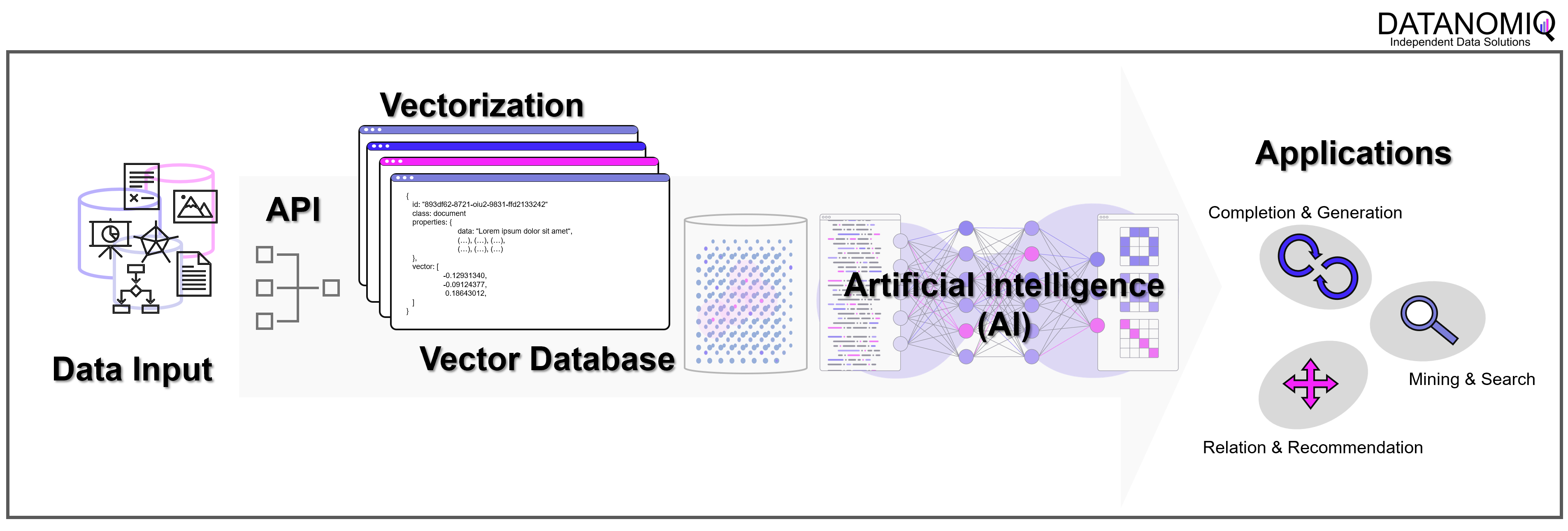
Ohne Vektor-Datenbanken wären die Erfolge von OpenAI und anderen Anbietern von LLMs nicht möglich geworden. Aber fernab der Entwicklung in San Francisco kann jedes Unternehmen unter Einsatz von Vektor-Datenbanken und den APIs von Google, OpenAI / Microsoft oder mit echten Open Source LLMs (Self-Hosting) ein wahres Orakel über die eigenen Unternehmensdaten herstellen. Dazu werden über APIs die Embedding-Engines z. B. von OpenAI genutzt. Wir von DATANOMIQ nutzen diese Architektur, um Unternehmen und andere Organisationen dazu zu befähigen, dass kein Wissen mehr verloren geht.
Vektor-Datenbank für KI-Applikation (z. B. OpenAI ChatGPT)

Mit der DATANOMIQ Enterprise AI Architektur, die auf jeder Cloud ausrollfähig ist, verfügen Unternehmen über einen intelligenten Unternehmens-Repräsentanten als KI, der für Mitarbeiter relevante Dokumente und Antworten auf Fragen liefert. Sollte irgendein Mitarbeiter im Unternehmen bereits einen bestimmten Vorgang, Vorfall oder z. B. eine technische Konstruktion oder einen rechtlichen Vertrag bearbeitet haben, der einem aktuellen Fall ähnlich ist, wird die AI dies aufspüren und sinnvollen Kontext, Querverweise oder Vorschläge oder lückenauffüllende Daten liefern.

Die AI lernt permanent mit, Unternehmenswissen geht nicht verloren. Das ist Wissensmanagement auf einem neuen Level, dank Vektor-Datenbanken und KI.

Process Mining / Process Analytics

Ist Process Mining in Summe zu teuer?

Celonis, Signavio (SAP). UiPath, Microsoft, Software AG, Mehrwerk, process.science und viele weitere Process Mining Tool-Anbieter mehr… der Markt rund um Process Mining ist stark umkämpft. Trotz der hohen Vielfalt an Tools, gilt Process Mining in der Einführung und Durchführung als teuer. Viele Unternehmen verzeichnen zwar erste Erfolge mit dieser Analysemethodik und den dafür geschaffenen Tools, hadern jedoch mit den hohen Kosten für Lizensierung und Betrieb.

Process Mining / Process AnalyticsDabei gibt es viele Hebel für Unternehmen, die Kosten für diese Analysen deutlich zu reduzieren, dabei gesamtheitlicher analysieren zu können und sich von einzelnen Tool-Anbietern unabhängiger zu machen. Denn die Herausforderung beginnt bereits mit denen eigentlichen Zielen von Process Mining für ein Unternehmen, und diese sind oft nicht einmal direkt finanziell messbar.

Process Mining bitte nicht nur auf Prozesskosten reduzieren

Tool-Anbieter werben tendenziell besonders mit der potenziellen Reduktion von Prozesskosten und und mit der Working Capital Optimierung. Bei hohen Lizenzierungskosten für die Tools, insbesondere für die Cloud-Lösungen der Marktführer, ist dies die erfolgversprechendste Marketing-Strategie. Typische Beispiele für die Identifikation von Kostensenkungspotenzialen sind Doppelarbeiten und unnötige Prozessschleifen sowie Wartezeiten in Prozessen. Working Capital- und Cash- Kosten sind in den Standardprozessen Order-to-Cash (z. B. Verspätete Zahlungen) und Procure-to-Pay (z. B. zu späte Zahlungen, nicht realisierte Rabatte) zu finden.

Diese Anwendungsfälle sind jedoch analytisch recht trivial und bereits mit einfacher BI (Business Intelligence) oder dedizierten Analysen ganz ohne Process Mining bereits viel schneller aufzuspüren. Oft bieten bereits ERP-Systeme eine eigene Erkennung hierfür an, die sich mit einfach gestrikter BI leicht erweitern lässt.

Richtige Wirkung, die so eigentlich nur Process Mining mit der visuellen Prozessanalyse erzeugen kann, zeigt sich vor allem bei der qualitativen Verbesserung von Prozessen, denn oft frustrieren eingefahrene Unternehmensprozesse nicht nur Mitarbeiter, Lieferanten und Partner, sondern auch Kunden. Dabei geht es z. B. um die Verbesserung von Prozessen in der Fertigung und Montage, in der Logistik, dem Einkauf, Sales und After Sales. Diese Anwendungszwecke dienen zur zeitlichen Beschleunigung oder Absicherung (Stabilisierung) von Prozessen, und damit zur Erhöhung des Kundennutzens. Jede qualitative Verbesserung wird sich letztendlich auch im quantitativen, finanziellen Maße auswirken, wenn auch nicht so einfach messbar.

Die Absicherung von Prozessen aus der Compliance-Perspektive ist eines der typischen Einsatzgebiete, für die Process Mining prädestiniert ist. Audit Analytics und Betrugserkennung gehören zu den häufigsten Anwendungsgebieten. Das senkt zwar grundsätzlich keine Prozesskosten, ist jedoch in Anbetracht immer komplexerer Prozessketten bittere Notwendigkeit.

Prozess Mining kann ferner auch zur Dokumentation von Geschäftsprozessen genutzt werden, als Vorlage für Sollprozesse. Die Analyse von bestehenden Prozessen kann dann dabei helfen, den aktuellen Zustand eines Prozesses zu dokumentieren und Unternehmen können diese Informationen nutzen, um Prozessdokumentationen zu aktualisieren und zu verbessern. Mit Process Mining können Vor- und Nachher-Vergleiche durchgeführt sowie situative Worst- und Best-Practise herausextrahiert werden. Dies bietet sich insbesondere vor und nach Migrationen von ERP-Systemen an.

Process Mining muss nicht (zu) teuer sein

Bei hohen Kosten für Process Mining ist der Druck einer Organisation sehr hoch, diese Kosten irgendwie mit hohen potenziellen (!) Einsparungen zu rechtfertigen. Die Prozesse mit dem höchsten Kostensenkungsversprechen erhalten dadurch den Vorzug, oft auch dann, obwohl andere Prozesse die nötige Prozesstransparenz eigentlich noch viel nötiger hätten.

Zumindest der Einstieg in Process Mining kann mit den richtigen Tools sehr leichtfüßig und günstig erfolgen, aber auch die Etablierung dieser Analysemethodik im weltweiten Konzern kann mit einigen Stellhebeln erheblich günstiger und (in Anbetracht der hohen Dynamik unter den Tool-Anbietern) nachhaltiger realisiert werden, als wie es von den größeren Anbietern vorgeschlagen wird.

Unabhängiges und Nachhaltiges Data Engineering

Die Arbeit hinter Process Mining kann man sich wie einen Eisberg vorstellen. Die sichtbare Spitze des Eisbergs sind die Reports und Analysen im Process Mining Tool. Das ist der Teil, den die meisten Analysten und sonstigen Benutzer des Tools zu Gesicht bekommen. Der andere Teil des Process Minings ist jedoch noch viel wesentlicher, denn es handelt sich dabei um das Fundament der Analyse: Die Datenmodellierung des Event Logs. Diese Arbeit ist der größere, jedoch unter der Oberfläche verborgene Teil des Eisbergs.

Jedes Process Mining Tool benötigt pro Use Case mindestens ein Event Log. Dabei handelt es sich um ein Prozessprotokoll mit universeller Mindestanforderung: Case, Activity, Timestamp

Diese Event Logs in einem Process Mining Tool zu modellieren und individuell anzupassen, ist langfristig keine gute Idee und erinnert an die Anfänge der Business Intelligence, als BI-Analysten Daten direkt in Tools wie Qlik Sense oder Power BI luden und für sich individuell modellierten.

Wie anfangs erwähnt, haben Unternehmen bei der Einführung von Process Mining die Qual der Wahl. Oft werden langwierige und kostenintensive Auswahlprozesse für die jeweiligen Tools angestoßen, damit die Wahl auf der augenscheinlich richtige Tool fällt.

Eine bessere Idee ist es daher, Event Logs nicht in einzelnen Process Mining Tools aufzubereiten, sondern zentral in einem dafür vorgesehenen Data Warehouse zu erstellen, zu katalogisieren und darüber auch die grundsätzliche Data Governance abzusichern. Die modellierten Daten können dann jedem Process Mining Tool zur Verfügung gestellt werden. Während sich Process Mining Tools über die Jahre stark verändern, bleiben Datenbanktechnologien für Data Warehousing über Jahrzehnte kompatibel und können in ihnen aufbereitete Event Logs allen Tools zur Verfügung stellen. Und übrigens lässt sich mit diesem Ansatz auch sehr gut eine gesamtheitlichere Verknüpfung realisieren und die Perspektive dynamisch verändern, was neuerdings als Object-centric Process Mining beworben wird, mit der richtigen Datenmoedellierung in einem Process Mining Data Warehouse für jedes Tool zu erreichen ist.

Nicht alles um jeden Preis in die Public Cloud

Unter der häufigen Prämisse, dass alle ERP-Rohdaten in eine Cloud geladen werden müssen, entstehen Kosten, die durchaus als überhöht und unnötig angesehen werden können. Daten-Uploads in eine Cloud-Lösung für Process Mining sollten nach Möglichkeit minimal ausfallen und lassen sich durch genaueres Anforderungsmanagement in den meisten Fällen deutlich reduzieren, verbunden mit Einsparungen bei Cloud-Kosten. Idealerweise werden nur fertige Event-Logs bzw. objekt-zentrische Datenmodelle in die Cloud geladen, nicht jedoch die dafür notwendigen Rohdaten.

Für besonders kritische Anwendungsfälle kann es von besonderem Stellenwert sein, einen Hybrid-Cloud-Ansatz anzustreben. Dabei werden besonders kritische Daten in ihrer granularen Form in einer Private Cloud (i.d.R. kundeneigenes Rechenzentrum) gehalten und nur die fertigen Event Logs in die Public Cloud (z. B. Celonis Process Mining) übertragen.

Mit AI ist mehr möglich als oft vermutet

Neben den einfachen Anwendungsfällen, die einige Tool-Anbieter bereits eingebaut haben (z. B. Matching von Zahlungsdaten zur Doppelzahlungserkennung oder die Vorhersage von Prozesszeiten), können mit Machine Learning bzw. Deep Learning auch anspruchsvollere Varianten-Cluster und Anomalien erkannt werden.

Unstrukturierte Daten können dank AI in Process Mining mit einbezogen werden, dazu werden mit Named Entity Recognition (NER, ein Teilgebiet des NLP) Vorgänge und Aktivitäten innerhalb von Dokumenten (z. B. Mails, Jira-Tickets) extrahiert und gemeinsam mit den Meta-Daten (z. B. Zeitstempel aus dem Dokument) in ein strukturiertes Event Log für Process Mining transformiert. Ähnliches lässt sich mit AI für Computer Vision übrigens auch auf Abläufe aus Videoaufnahmen durchführen. Dank AI werden damit noch viel verborgenere Prozesse sichtbar. Diese AI ist in noch keiner Process Mining Software zu finden, kann jedoch bausteinartig dem Process Mining Data Warehouse vorgeschaltet werden.

Fazit

Nicht all zu selten ist Process Mining den anwenden Unternehmen in Summe zu teuer, denn bereits einige Unternehmen sind über die Kosten gestolpert. Andere Unternehmen begrenzen die Kosten mit dem restriktiven Umgang mit Benuter-Lizenzen oder Anwendungsfällen, begrenzen damit jedoch auch den Analyseumfang und schöpfen nicht das volle Potenzial aus. Dies muss jedoch nicht sein, denn Kosten für Data Loads, Cloud-Hosting und Benutzerlizenzen für Process Mining lassen sich deutlich senken, wenn Process Mining als die tatsächliche Analyse-Methode verstanden und nicht auf ein bestimmtes Tool reduziert wird.

Zu Beginn kann es notwendig sein, Process Mining in einer Organisation überhaupt erst an den Start zu bringen und erste Erfolge zu erzielen. Unternehmen, die Process Mining und die damit verbundene Wirkung in Sachen Daten- und Prozesstransparenz, erstmals erlebt haben, werden auf diese Analysemethodik so schnell nicht mehr verzichten wollen. Schnelle erste Erfolge lassen sich mit nahezu jedem Tool erzielen. Nach Pilot-Projekten sollte der konzernweite Rollout jedoch in Sachen Performance, Kosten-Leistungsverhältnis und spätere Unabhängigkeit überdacht werden, damit Process Mining Initiativen langfristig mehr wirken als sie kosten und damit Process Mining auch bedenkenlos und ohne Budget-Engpässe qualitative Faktoren der Unternehmensprozesse verbessern kann.

Mit den richtigen Überlegungen fahren Sie die Kosten für Process Mining runter und den Nutzen hoch.

Praxisbeispiel: Data Science im Marketing

Wie Sie mit Data Science die Conversion-Rate in Ihrem Online-Shop erhöhen

Die Fragestellung: Ein Hersteller von Elektrogeräten lancierte einen neuen Online-Shop, um einen neuen Vertriebskanal zu schaffen, der unabhängig von stationären Einzelhändlern und Amazon ist. Obwohl der Online-Shop von Interessent:innen häufig besucht wurde, war die Conversion-Rate zu niedrig und der Umsatz somit zu gering.

Die zentrale Frage war nun: Wie kann die Conversion-Rate erhöht werden, um den Umsatz über den neuen Vertriebskanal zu erhöhen?

Was ist eine Conversion-Rate? Die Conversion-Rate ist eine Marketing-Kennzahl, die in diesem Beispiel das Verhältnis der Besucher:innen des Online-Shops zu den getätigten Käufen meint. Halten sich viele Besucher:innen im Online-Shop auf und sind die Warenkorb-Abschlüsse dennoch gering, so ist die Conversion-Rate niedrig. Das Ziel ist es, die Conversion-Rate zu steigern, also dafür zu sorgen, dass Besucher:innen, die sich im Online-Shop befinden und dort etwas in den Warenkorb legen, auch einen Kauf tätigen.

VorgehenUm zu verstehen, warum eine Bestellung abgeschlossen bzw. nicht abgeschlossen wurde, wurden verschiedene Daten aus dem Web-Analytics-System des Online-Shops untersucht. Dazu gehörten im Wesentlichen Daten zu Besucherhandlungen auf der Website, die automatisch getrackt, also aufgezeichnet werden, wie z. B. Button & Link-Klicks, Bildergalerie öffnen, Produktvideo ansehen, Produktbeschreibung ausklappen, Time on page usw.

Mit diesen Daten wurden drei Analyseverfahren durchgeführt.

1) Website-Besucher verstehen

Zunächst wurden mit einer explorativen Datenanalyse die Website-Besucher:innen und deren Bedürfnisse untersucht. Über die meisten der Besucher:innen lagen bereits Daten vor, da sie in der Vergangenheit bereits Käufe auf der Website getätigt hatten und dafür ein Konto angelegt hatten. Darüber hinaus wurde untersucht, über welche Kanäle die Besucher:innen in den Online-Shop gelangten, beispielsweise über Google oder Facebook. Informationen zu Gerät, Standort, Browser und Betriebssystem waren ebenfalls verfügbar.

Anhand dieser unterschiedlichen Parameter wurden die Benutzerdaten einem Analyseverfahren, dem sog. Clustering, unterzogen, bei dem die Website-Besucher:innen aufgrund ihrer Ähnlichkeiten in verschiedenen Eigenschaften in Gruppen („Cluster“) eingeteilt wurden.

Beispiel: Besucher über Android-Smartphones und Chrome-Browser, die zwischen 17 und 19 Uhr am Samstag auf der Website sind, kaufen eher familienbezogene Produkte.

Daraufhin konnte man neue Website-Besucher:innen aufgrund der verschiedenen Eigenschaften meist recht eindeutig einem Cluster zuordnen, da ähnliche Besucher:innen tendenziell ein ähnliches Verhalten auf einer Website zeigen. Dieses Clustering lieferte dem Unternehmen bereits wertvolle Informationen. So konnten auf dieser Informationsgrundlage individuelle Marketingstrategien für verschiedene Zielgruppen entwickelt, das Werbe-Targeting angepasst und spezifische Sonderangebote erstellt werden.

Beispiel: Besucher über Android-Smartphones und Chrome-Browsern, die zwischen 17 und 19 Uhr am Samstag auf der Website sind, bekommen ein Sonderangebot für ein familienbezogenes Produkt, wie beispielsweise ein Babyfon ausgespielt.

In vielen Fällen reicht eine solche Analyse bereits aus, um die Conversion-Rate eines Online-Shops spürbar zu steigern. In diesem Projekt wurden jedoch noch zwei weitere Analyseschritte durchgeführt.

2) Conversion Path verstehen und Engpässe nachvollziehen

Der nächste Schritt bestand darin, den Conversion Path der Kund:innen zu untersuchen. Der Conversion Path umfasst alle Handlungen von Kund:innen vom Ankommen auf der Website über den Besuch verschiedener Seiten bis hin zum finalen Kauf bzw. Kaufabbruch. Bei der Analyse wurden alle Conversion Paths auf Gemeinsamkeiten und Unterschiede untersucht, um bestimmte Muster abzuleiten. Von besonderem Interesse waren mögliche Gründe, aus denen Besucher:innen ihre Sitzung vor Kaufabschluss abbrachen. Es stellte sich heraus, dass Besucher:innen ihre Sitzung vor allem dann abbrachen, wenn es für ein Produkt kein Produktvideo gab bzw. das Produktvideo nicht gefunden wurde. Diese mangelnde Produktinformation konnte anschließend gezielt bearbeitet werden, woraufhin sich die Conversion-Rate deutlich verbesserte.

3) Next-best-Action vorhersagen

Im dritten Schritt des Projektes zur Steigerung der Conversion-Rate wurde der Ansatz der Next-best-Action (NBA) gewählt. Damit wurde hier ein weiterer Schritt von der reinen Analyse von bereits vorhandenen Daten hin zur Vorhersage zukünftigen Verhaltens gewählt.

Was bedeutet Next-best-action? Next-best-action (NBA) ist eine Marketingstrategie, die darauf abzielt, Informationen über einzelne Kund:innen zu sammeln und zu nutzen, um einen Kauf anzuregen. Wie der Name schon sagt, wird versucht zu ermitteln, welcher der nächste beste Schritt im Verkaufsprozess für jede:n einzelne:n Kunde:in ist.

Mithilfe der allgemeinen Informationen über die Website-Besucher:innen und der Conversion Paths konnten unterschiedliche Aktionen identifiziert werden, die einen Kauf wahrscheinlicher machen würden. Dazu gehörte z. B., den Besucher:innen das Produktvideo anzuzeigen, einen Rabatt-Code oder ein Sonderangebot für eine spezielle Produktkategorie anzubieten oder ein Chat-Fenster für den Kundensupport zu öffnen.

Somit half die NBA-Vorhersage dabei, die Conversion erneut deutlich zu steigern, indem für jede:n Website-Besucher:in eine individuelle Aktion vorgeschlagen werden konnte.

Ergebnisse:

In diesem Projekt konnte die Marketingabteilung des Elektrogeräte-Herstellers durch drei verschiedene Analyseansätze die Conversion-Rate im Online-Shop deutlich verbessern:

  • Mithilfe des Clustering war das Unternehmen in der Lage, individuelle Marketingstrategien für verschiedene Zielgruppen zu entwickeln, das Werbe-Targeting anzupassen und spezifische Sonderangebote zu erstellen.
  • Durch die Analyse der Conversion Paths konnten produkt- und produktbeschreibungsspezifische Engpässe identifiziert und anschließend gezielt behoben werden.
  • Mit der NBA-Analyse konnten nächste beste Schritte für jede:n einzelne:n Kunde:in bestimmt und automatisch ausgelöst werden.

How to tackle lack of data: an overview on transfer learning

1, Data is the new oil, but labeled data might be closer to it

Even though we have been in the 3rd AI boom and machine learning is showing concrete effectiveness at a commercial level, after the first two AI booms we are facing a problem: lack of labeled data or data themselves. The increasing number of papers on deep learning demonstrate that researches on AI have developed rapidly recently. If architectures of neural networks and supervised learning are all you know about deep learning, you will be overwhelmed by complications of topics studied these days, for example generative models, making more compact neural net models by for example knowledge distillation, and explainable AI (XAI). Those researches are often conducted on easily available benchmark datasets which you can easily download, often with corresponding ground truth data (label data) necessary for training. However once you try to apply the techniques to more specific data, you usually cannot prepare enough label data which theoretical researches assume. Thus among fascinating deep learning topics, in this article I am going to pick up how to tackle lack of label or data themselves, and transfer learning. Transfer learning is a technique of machine learning to take advantages of knowledge learned in one dataset to deal with a task in another dataset. Presumably due to this fact, Andrew Ng, in his presentation in NeurIPS 2016, gave a rough and abstract predictions of how transfer learning in machine learning would make commercial success like white lines in the figure below. The explanation is straightforward, and given the trends in topics of researches on machine learning these days, this prediction is actually right. But at the same time, in my opinion supervised learning, transfer learning, and unsupervised learning cannot be clearly separated like the graph originally suggested by Andrew Ng. Those fields complement each other, and one can easily shift to another.
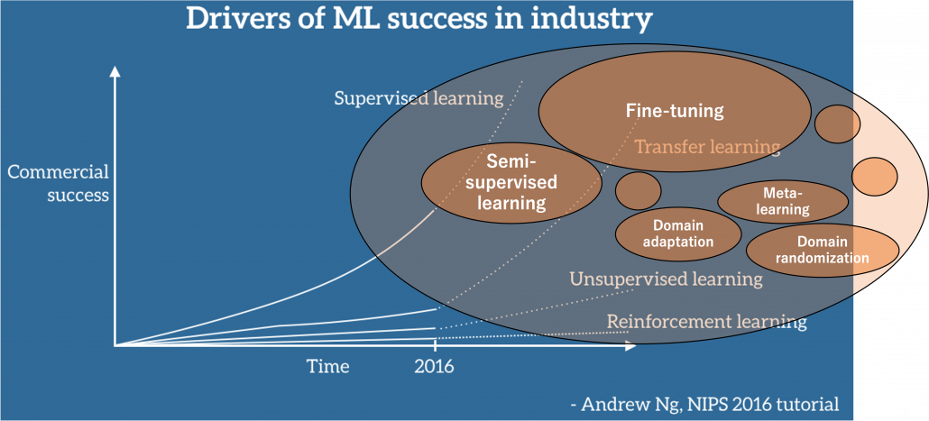
Source: https://ruder.io/transfer-learning/ The lines and texts in white are based on explanations by Andrew Ng. The orange cells are placed at random, so not that they represent commercial success of each field.

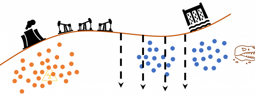
Along with the rapid progress of deep learning mentioned above, a lot of hypes and catchphrases regarding big data and machine learning were made, and an interesting one is “Data is the new oil.” That might have been said only because big data is sources of various industries. But I would say, the characteristic is more striking in training data for machine learning. Distributions of training data for machine learning are more complicated like various energy resources besides oil in the world. Labeled data might be also like uranium. Just as uranium-235 accounting for only less than one percent of uranium in the world can be used to generate energy, only a part of massive data in the world is labeled such that they can be used for supervised machine learning. And as uranium-235 is used effectively jointly with less active uranium-238, labeled data show greater potentials with unlabeled data. And training data for machine learning have another unpleasant analogy to energy resources. Like most mainstream energy resources, only limited companies or institutions would be able to mine and refine huge labeled datasets with gigantic computation resources, and most people more or less need to rely on that for their business. Even though alternative renewable energy resources are proposed, principal energy resources are indispensable for making industries stable. As well, even though a lot of techniques actually have been proposed to lack of data, it often turns out just fine-tuning pre-trained models is the most practical, which need huge datasets and rich computational resources. And I think recent success in for example BERT or GPT made this trend more visible.

*I am sorry in a case I am mistaken about energy resources. I just wanted to come up with some cool metaphors.

But I still think knowing about transfer learning more comprehensively would be effective. That is partly because I have been working on relatively unique data which are hard to even label. As I was studying computer vision (CV) in plant science field, I frequently saw relatively unique data obtained with special apparatuses. Such data are for the most part look far from very general dataset, which huge pre-trained models are trained on. At the same time such plant data have very complicated structures and hard to label. And also in my work, have to detect certain values in various formats in very specific documents, in German. Such data are far from general datasets, and even labeling is hard in that case. We have to carefully tackle lack of data every time on each type of data in that case.

In this article I would first like to explain in the first place what it is like to lack data and next introduce representative techniques to tackle lack of labeled data. Many of them are classified to transfer learning, but other techniques like unsupervised learning or self-supervised learning are used in them or share a lot in their ideas. Thus my main purpose of writing this article is to let you have a richer view on transfer learning. And you would see “transfer learning” these days are mainly about fine-tuning of pre-trained models. Also how to tackle lack of data or labels is in other words how to efficiently achieve good performance in machine learning. Thus even if tons of high quality labeled data are at your disposal, learning those ideas would be still effective to you. I hope you could find some hints of machine learning through my articles.

2, What does lack of data or labels mean in the first place?

We need to first consider what lack of labels or data means, and my answer to the title of this section is “It depends.” The more data you have, the better performances you get. And the bigger machine learning models are, the more data they usually need for training. I assume that people reading this article more or less understand neural networks and how they are trained with back propagation. But let’s review the process here. Most machine learning frameworks are more or less expressed like the figure below unless reinforcement learning is considered. The ultimate purpose of machine learning is to train a model f(\boldsymbol{x}_n;\boldsymbol{\theta}) by adjusting parameters \boldsymbol{\theta}. And the parameters \boldsymbol{\theta} are optimized so that a loss function L is minimized. If it is a supervised learning, the a value of a loss function is denoted L(f(\boldsymbol{x}_n, \boldsymbol{\theta}), \boldsymbol{y}_n) =L(\hat{\boldsymbol{y}}_n, \boldsymbol{y}_n), and it gets smaller as f(\boldsymbol{x}_n, \boldsymbol{\theta}) gets closer to \boldsymbol{y}_n. That is, \boldsymbol{y}_n is giving supervision to adjust f(\boldsymbol{\theta}) via L(\hat{\boldsymbol{y}}_n, \boldsymbol{y}_n). And in a case of unsupervised learning, a loss function is L(\hat{\boldsymbol{y}}_n), which is often heuristically handcrafted.

The very first problem from lacking training data you would learn is overfitting. That is, a machine learning model can be specialized too much for a training dataset, and it loses generalization to other data from the same dataset. It is like students with little imaginations and flexibility gradually memorizing all the answers in a textbook and failing to answer new questions they have not encountered yet. Overfitting is judged by relations of training and validation loss like in the graph below. Training loss in blue indicates how the students adjust to the textbook. The smaller the training loss is, the more they memorizes from the textbook and the less flexible they are. The orange line indicates their performance in newly appeared questions in tests. The smaller the validation loss is, the better the students perform on tests. Thus the students should stop learning with the textbook when the validation loss is about to increase. This is called early stopping in machine learning. And if you increase training data, the orange graph usually shifts to the right side, usually providing smaller validation loss, namely better performance. An important point is, this ideal relations of training and validation losses will not appear if sizes or expressivity of a model is not enough. Thus the more training data you use, the more parameters you need for the model to enhance its expressivity.
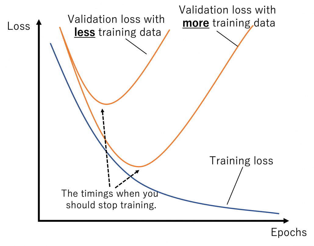
 

*Depending on sizes of training data, the curve of training loss also changes, so please bear it in mind that this graph is not correct and is very simplified.

What I said so far might sound too elementary. My point is, the more data you have, and the bigger computation resource you have, the better performance you get. In other words, machine learning has scalability with data and parameters. This characteristic is clearly observed in models in natural language processing (NLP) and computer vision (CV) like in the graphs below. When I read some papers,often I am very fascinated by their performances. But sometimes it turns out that the methods are mainly creatively in terms of how they increase training data, which is personally boring. And even if performance of GPT looks astonishing, I cannot really like them because of this simple fact.
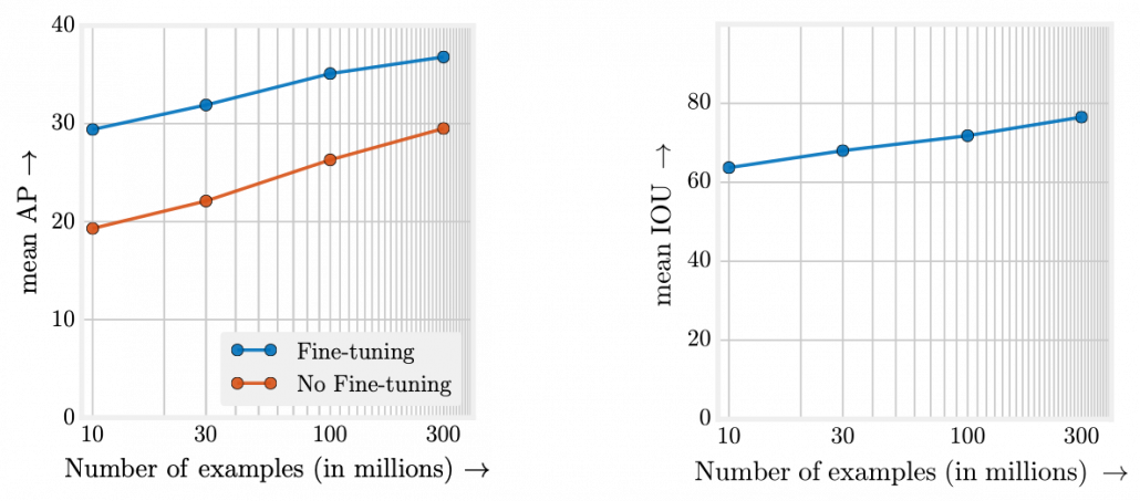
However another important point is, conversely you don’t need to increase training data or parameters of a model once it achieves an ideal score in metrics. When you make a toy model with small training data, as long as your clients or co-researchers are already happy, that is enough. Therefore lack of data or labels has to be discussed depending on sizes of machine learning and their performances you expect. Given those points mentioned so far, my answer to the question “What does lack of data or labels mean?” would rephrased like “If your model is properly designed to reach the performance you expect and it starts overfitting, you are facing lack of data.” And such decisions basically has to be made based on experiments.

3, Types of lack of data

Even though I explained lack of labels or data is a contextual matter, the problems actually exist at any case. That is, you often fail to achieve ideas accuracy partly due to lack of training data. I would like to classify types of situations of data of label shortage as below.

We should first think about the case where lack of labels does not matter in the first place. If you can analyze data with statistical knowledge or unsupervised machine learning, just extracting data without labeling would be enough. And sometimes ad hoc analysis with simple data visualization will help your decision makings. And some dashboards made from those unlabeled data will already give you some insights into data.

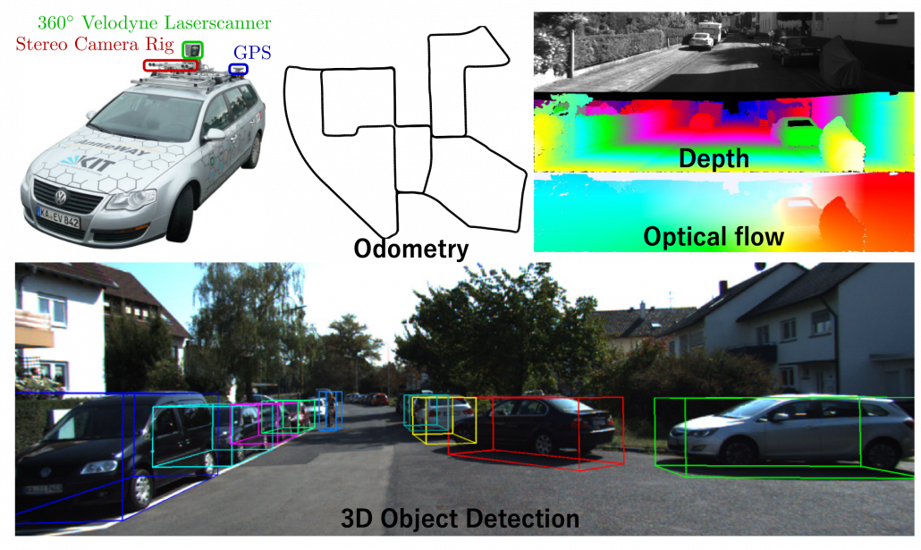
The next case is that, popular machine learning fields with enough investments usually have huge datasets that huge academic institutes or companies have been preparing.  For example KITTI dataset, which include labels like trajectories and depth data, is by Karlsruhe Institute of Technology and Toyota Technological Institute. Such datasets are useful for self-driving-related researches, and many types of ground truth data are provided such as odometry, depth, opticla flow, detection. This kind of data might be considered “enough” only because they are enough for training machine learning models and quantitatively evaluating them in papers, regardless of practical usefulness at a commercial level. But at any rate, popular fields with large benchmark datasets are likely to get investments for commercial uses.
Next let’s see cases of data shortage. You should also keep it in mind that there are also several types of situations of data shortage. In fact there are cases where certain labels are supposed to be scarce such as classifications of imbalanced data, for example anomaly detection, judging spam mails,  or medical examination. In those problems only some percent of data are classified as “errors,” “spam,” or “disease,” and others are classified as “normal.” Just keeping classifying data into “normal” would give maybe more than 95% accuracy. But finding the rest some percent accurately is much more important. In this case model performances need to be evaluated with ROC curves, namely relations of true positives and false positives.

The next type is more related to cases assumed in transfer learning. Some data are in the first place very expensive to obtain. For example CT images have to be stored by special medical apparatuses as you know. And even if a lot of CT images are already obtained, annotating the images often needs professional skills, thus its annotations cost is high. Another case of high annotation cost is for example detection or segmentation of objects in images. Even if you can collect numerous images on the Internet, annotating bounding boxes or pixel-wise segments require a lot of time. Annotating around 1000 images  for classification might be ok, but annotating them at a pixel level is really time consuming. If you have a tablet, I would like you to paint each segment of objects in a picture with different colors. And you should multiply the time spent by 80,000, as many as the training images needed for Mask R-CNN, a popular model for instance segmentation. As you can imagine, it is a huge tediou work. Even preparing some 50 labeled images for fine-tuning is paiful, and even annotations for computer vision tasks itself is also a field of deep learning.

*I would say medical image processing is a relatively popular field in CV with deep learning, and there are several famous datasets on this field.

4, An overview on ways for dealing with lack of labeled data

I am going to first roughly introduce what kind of approaches can be taken to deal with lack of labeled data or data itself, but you should also keep it in mind that they are not clearly separated. Just as I am going to explain, one type of techniques can easily shift to another type. You should flexibly switch among them depending on your situations. And also please keep it in mind that these are well-studied areas, and tons of ingenious papers are announced one after another, usually giving slight changes in their performances. Problems I point out about each technique might not be a problem anymore with recently published researches on researches currently peer-read. It is hard to prove that something does not exist. Given those points, I think it is convenient to classify technique of dealing with label or data shortage as below.

Through this article, ideas of domains are important. A domain simply means a combination of a dataset and a task with it. Transfer learning is a family of machine learning techniques to make uses of knowledge learned in a domain to another domain, and the former is called a source domain, the latter a target domain. And discrepancies between a source domain and a target domain is called a domain shift. The figure below abstractly visualize examples of domains and domain shifts. Intuitively it is easy to imagine that face a CV task and an NLP task have bigger domain shifts than domains of leaf images taken from different angles, but quantitatively evaluating domain shifts is in practice hard, and I am not going to introduce the topic because that will need a lot of mathematics.

Instead of formulating transfer learning, I would like to take learning languages as an intuitive example of transfer learning. Most people master at least one native language before learning another one. Baby brains are a kind of fantastic machine learning models, and after overcoming many obstacles they master native languages. And people take advantages of their mother tongues to learn another language. Usually they learn foreign languages by comparing structures of translated sentences. And naturally, if both a foreign language and your language have analogies like grammatical cases or genders in common, language learning would be easy. In other words, proficiency in one language is helpful in leaning some language. But it is also possible that your native language badly affects learning the second language, due to grammatical structures, pronunciations. The case of a source domain deteriorating performances in a target domain is called negative transfer and contexts of transfer learning.

*I know similarities languages are not the sole and definite barometers of effectiveness in learning foreign languages. Sizes of economy or markets in a country would also affects English language acquisition of people there. But at least it is unfair to compare for example German or Dutch people learning English with Japanese, Chinese people learning it. Unlike Eastern Asian people who have to learn thousands of characters to at least read decent texts or who use very different grammars, European people obviously can use “transfer learning” to learn English.

5, Increasing training data

When you lack data or labels, the most straightforward and often quick solution is to just increase data. The two topics I will cover in this section are mainly conducted in one domain.

Data augmentation

Data augmentation is one of the first techniques you would learn to mitigate overfitting of machine learning, which is in short caused by lack of data. The idea is very simple and it is implemented well in deep learning libraries, so I would only briefly talk about it here. The idea of data augmentation is simply transforming input data by for example flipping, rotating, zooming, changing colors. By doing so for example an input image \boldsymbol{x}_n of a butterfly below with a label of \boldsymbol{y}_n = \text{Butterfly} can be converted to more than 6 images. This corresponds to getting a converted \boldsymbol{x}'_n= g(\boldsymbol{x}_n) in the machine learning outline in the last section. And this process is the same as increasing the size of a dataet \mathcal {D}. And one point you have to be careful is, you must not change \boldsymbol{x}_n too much to change corresponding \boldsymbol{y}_n. For example if \boldsymbol{x}_n is distorted too much, it cannot be recognized as \boldsymbol{y}_n anymore even by humans. Or if you rotate an image of a digit 6 180 degrees, its becomes 9. Recent researches focus on automatically find what kind of data augmentation is effective by using for example reinforcement learning.

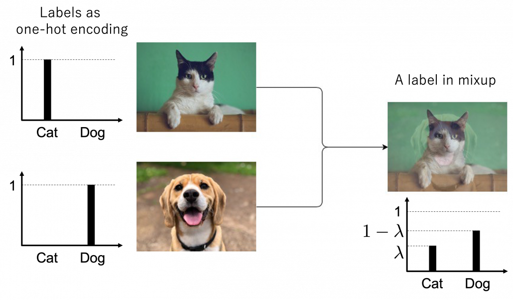
Here let me take an example of data augmentation technique that would be contrary to your intuition. A technique named mixup literally mix up data with different classes and their labels. In classification problems, labels are expressed as one-hot vectors, that is only an element corresponding to a correct element is 1 and the others are 0. In a case of binary dog-or-cat classification, each label is \boldsymbol{y}_n = (1, 0)^T or \boldsymbol{y}_n = (0, 1)^T, respectively. In data augmentation, distorting data too much is a taboo because label data is contaminated, but in mixup you literally mix up labels. Randomly choosing a two inputs \boldsymbol{x}_n , \boldsymbol{x}_{n'} and a  number \lambda \in [0,1], you prepare a input and label pair (\lambda \boldsymbol{x}_n + (1 - \lambda) \boldsymbol{x}_{n'},  \lambda \boldsymbol{y}_n + (1 - \lambda) \boldsymbol{y}_{n'}). The figure below is an example of a mixing up a cat input and a dog input, and corresponding labels. It is known augmenting training data like this improves classification performances. It is said this is partly due to machine learning models effectively learning decision boundaries. In classification ambiguous inputs are bottlenecks, so learning to giving ambiguous outputs to ambiguous inputs can enhance classification abilities.
*One-hot-encoded labels are called hard labels, and otherwise soft labels. Recent topics in deep learning, such as lottery hypothesis, knowledge distillation, imply that whether supervising labels are hard or not is important in deep learning. Hopefully I would like to explain why little by little in my articles.

6, Active learning

Active learning is about how to annotate data and get labeled data efficiently. Labels of data do not equally contribute to enhancing machine learning models, and labels actually have qualities. Even if you give apparently similar images with the same label to machine learning models during training, the models cannot learn so much from the pair of data. You need to efficiently dig data to know its distribution by giving labels to samples. I think a good metaphor is geological survey by excavating with some boring. In order to know substances or features of ground, some earth need to be sampled with boring. But you cannot freely penetrate everywhere mainly due to costs. They need to be sampled one by one due to uncertainty about the ground.
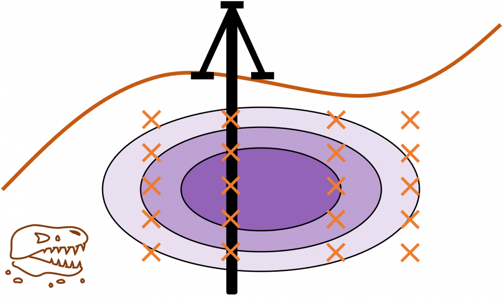
 

Similar approaches are often taken in machine learning or statistics, that is estimating distributions of data with a small size of samples is an important idea. A basic idea for doing that is you sample or annotate data which decreases uncertainty of your model the most. The figure simply exhibits the idea. We want to regress a data distribution with the red curve, and the cross marks can be sampled from the distribution. And the part filled with light blue shows uncertainty of the model to predict a value of y for a x. When you want to regress the data with as few samples as possible, data points should be sampled from the parts with great uncertainties. And by doing so, you can see that the data is regressed efficiently with few samples.
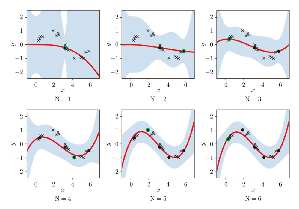
We have seen that modeling uncertainty is the key to active learning, and that can be applied to annotations of data in deep learning. An example of the process is displayed below, and in this case a deep neural network model (DNN model) is trained with some labeled data, and you give some signals for data annotations based on uncertainty of outputs of DNN models. And human annotators prioritize giving labels to the data. Such uncertainly can be estimated by using entropy of outputs or modeling data distributions.
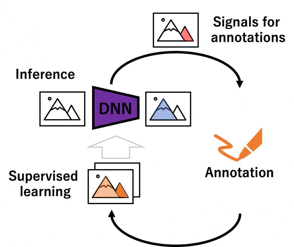
 

But when you get a certain amount of labels, the situation will be the same as semi-supervised learning, which I will explain next. That is, you might be already able to make the most of the labels so far with the help of unlabeled data. You should consider stopping labeling and start labeling depending on situations. And importantly, starting naively annotating data might become a quick solution rather than thinking about how to make uses of limited labels if extracting data itself is easy and does not cost so much. “Shut up and annotate!” could be often the best practice in practice. And annotations would be an effective way for exploratory data analysis (EDA), so I recommend you to immediately start annotating about 10 random samples at any rate.

7, Dealing with lack of labels in a single domain

In many cases, data themselves are easily available, and only annotations costs matter. The following two topics consider such cases, and again only one domain is considered. But by the end of this article you would see that other techniques covered in this article have a lot of analogies with topics introduced here.

Semi-supervised learning

Semi-supervised learning is a type of supervised learning where only limited labels are available in one domain. This is important in because many of other techniques in this article can be seen as semi-supervised learning from certain points of views. The figure below shows an intuition on semi-supervised learning in a case of classification task. In this case, original data distribution have two clusters of circles and triangles and a clear border can be drawn between them. But only with limited labeled data, decision boundaries would be ambiguous. However in fact, with a help of unlabeled data in dotted lines, machine learning model might be able to recognize two clusters with a help of unlabeled data. In other words, unlabeled data help models learn distribution of data. this might be natural as clusters of data can be estimated with unsupervised learning.
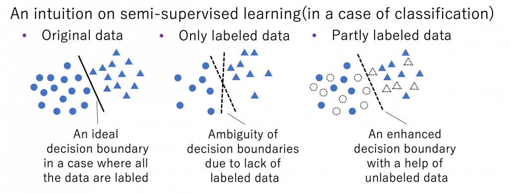
*As I have already mentioned, active learning could soon shift to semi-supervised learning, and it might be worth trying it before finishing labeling. But suspending labeling and resuming it later might not be efficient. At any rate you need to be flexible depending on situations.

Semi-supervised learning is applicable to several tasks, not only classification. I explained that normal supervised learning is adjusting parameters \boldsymbol{\theta} of a model f(\boldsymbol{\theta}) so that it minimize loss function L(\boldsymbol{\theta}, \mathcal{D}_{\text{L}}) for a labeled dataset \mathcal{D}_{\text{L}}. In semi-supervised learning, we assume that usually a bigger unsupervised dataset \mathcal{D}_{\text{UL}} is available in the same domain. And semi-supervised learning optimize \boldsymbol{\theta} by jointly minimizing L(\boldsymbol{\theta}, \mathcal{D}_{\text{L}}) + L'(\boldsymbol{\theta}, \mathcal{D}_{\text{UL}}) after designing a loss function L'(\boldsymbol{\theta}, \mathcal{D}_{\text{UL}}) for the unlabeled dataset. There are following 3 major ways of semi-supervised learning depending on how you design a L'(\boldsymbol{\theta}, \mathcal{D}_{\text{UL}}).

  • Consistency regularization: adding slight changes to data \boldsymbol{x}_{\text{UL}} in \mathcal{D}_{\text{UL}} and get \boldsymbol{x}'_{\text{UL}}. And training f(\boldsymbol{\theta}) so that f(\boldsymbol{\theta}, \boldsymbol{x}_{\text{UL}}) and f(\boldsymbol{\theta}, \boldsymbol{x}'_{\text{UL}}) give out a consistent output.
  • Pseudo label: after training f(\boldsymbol{\theta}) with \mathcal{D}_{\text{L}}, using some estimations f(\boldsymbol{\theta}, \boldsymbol{x}_{\text{UL}}) as labels of \mathcal{D}_{\text{UL}} .
  • Entropy minimization: encouraging outputs f(\boldsymbol{\theta}, \boldsymbol{x}_{\text{UL}}) to have smaller entropy.

More or less similar ideas show up in different transfer learning techniques, so it would be effective to learn the three semi-supervised learning ideas above.

Self-supervised learning

Self-supervised learning is often counted as unsupervised learning. Both unsupervised and self-supervised learning do not need label data, but especially when labels generated by processing themselves, that is often called self-supervised learning. A representative case of using self-supervised learning is auto-encoder. Simpler labels can be generated from input data themselves with elementary data processing. For example in a case of image processing, by rotating an input image 0, 90, 180, 270 degrees respectively, a classification task of estimating rotation degrees can be made. Another case is estimating the original input image after some simple image processing (for example colorization).  These simple tasks generated solely from an input is called pretext task. And in a case of image processing, deep learning models can be prompted to learn image features .

Source: https://atcold.github.io/pytorch-Deep-Learning/en/week10/10-1/

Pretext tasks are applicable also to other fields for example NLP. A very simple task is hiding a part of an input sentence, and let neural networks estimate the blank word. And this is a basic idea of how to train BERTs, famous pre-trained NLP models. BERT models are trained this way with a huge and very general corpus without any specific topics. By doing so BERT model can already learn to detect some clusters of meanings in texts, as I visualize in the next section. But if you fine-tune BERT models with labeled texts with very specific topics, that often fails to achieve satisfying performance. In that case, the BERT models have to “get used to” the new dataset. In that case, BERT can “get used to” the new dataset by applying self-supervised learning on the new dataset. This tutorial of Huggingface demonstrates this with an example of adjusting a BERT model trained with Wikipedia to the IMDb dataset.

In the case above, the BERT model is fine-tuned with relatively lots of unlabeled data and after that trained with fewer labels. As a whole this can be seen as semi-supervised learning ,with fewer labels of the IMBb dataset and more unlabeled data. Also the ideas of pretext tasks, which prompt models to give consistent outputs given preprocessed inputs, have some analogies with consistency regularization in semi-supervised learning.

*The Huggingface tutorial says, they fine-tune a pre-trained BERT model trained in a self-supervised way to adjus it, and they call it “domain adaptation.” As you can see from the statement, distinctions of topics covered in this article can be just ambiguous.

8, Dealing with lack of data or labels over several domains

Another approach for tackling label or data shortage is taking advantages of other domains, which are usually larger and have enough labels. And such techniques is called transfer learning as I mentioned. It seems like transfer learning in business refers to “fine-tuning” explained below, but in academic contexts it is often also said transfer learning is almost synonym to “domain adaptation.” At any rate, my point is it would be more important to have comprehensive view on the techniques rather than clearly distinguishing them.

Fine tuning

Fine tuning would be the easiest way of transfer learning, and at the same time it is very powerful. Even though I am going to introduce other technique of transfer learning, more often than not it turns out that fine tuning can compensate them. Here I will only explain what it is like to use fine-tuning. I would say using fine-tuning is easy like using instant coffee. Conventionally you needed to train your original model with your own data, and that is very affected by sizes of data you have. I would say, that was like making coffee or coffee cakes from coffee you made from beans. But by using pre-trained models already trained somewhere with huge datasets, you can use models which can already more or less recognize data. The idea was very normal already in the field of CV, and NLP got the same idea with the advent of BERT, or already with word embeddings. That is like people learned to use instant coffee instead of roasting and brewing coffee every time.
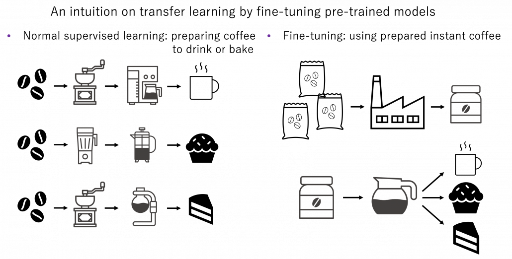
How such instant coffee is made depends on which type of deep learning is used on a huge dataset. Backbone CNN is usually trained on ImageNet dataset with supervised learning of a classification task. In case of BERT, it is trained with a huge corpus with a pretext task of estimating blank words of input sentences, which is classified to self-supervised learning. Let me more practically what the “coffee syrup” means. Machine learning is at any rate just mapping of tensors or vectors. In CV, an input images as a tensor is converted into a a vector or a tensor, and tasks like image classification are conducted with the converted tensor or vector. In case of an NLP task, usually a sequence of vectors is converted to a vector or another sequence of vectors. And these resulting tensors of vectors from models are the very “coffee syrup” I am talking about. An important point is, fine-tuning also considers transfer learning between different tasks. Backbone CNNs are usually trained with classification, BERT with self-supervised learning, but the there are a variety of final tasks. They are called downstream tasks. In other words, you don’t necessarily drink instant coffee as coffee.
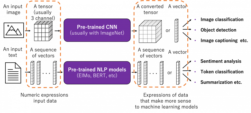
 

The two figures below are visualizations what the “instant coffee syrup” means. I processed random N images in a dataset with a pre-trained backbone CNN, and I got corresponding D dimensional vectors, that is a N\times D tensor. And I applied t-SNE to reduce its dimension from D to 2 and got a N\times 2 tensor.  The figure below shows arrangements of input images in the 2 dimensional space. As you can see, semantically similar images get closer.
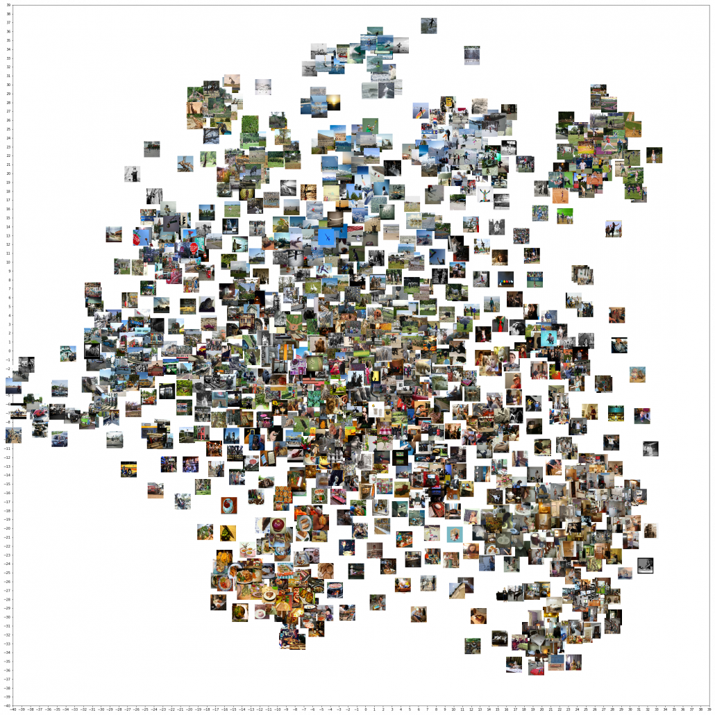
Just as well, if you process random texts with BERT and apply a dimension reduction, you get a visualization like below. As well as the figure above, texts in similar topic get closer.
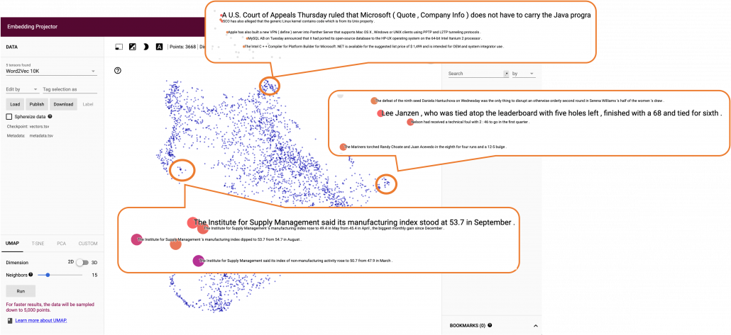
To make it catchy I expressed them as “coffee syrup” but this is a kind of how so-called AI sees data. Images and texts are just vectors or tensors on computer, and AI process another set of tensors of vectors in spaces which make sense to them.

Fine-tuning is quite easy. You have only to train a pre-trained model you downloaded just like normal supervised learning with your dataset. And when you train CV models with backbone CNN, the backbone is almost automatically downloaded. You have to be careful about some points, for example you have to set learning rate smaller. Let me avoid too detailed points in this article. Hopefully in the future, I’d like to write about more practical fine-tuning tips.

Domain adaptation

Domain adaptation is another family of techniques to make uses of knowledge gained in one domain in another domain. Domain adaptation is a Domain adaptation is these days often used as almost a synonym of transfer learning. But papers on domain adaptation usually assume to handle the same tasks both in a source and a target domain. So I would say domain adaptation is a subfield of transfer learning. Domain adaptation is more of how to tackle deterioration of machine learning performances when trained models are applied in different domains. Based on how much labels are available in each domain, domain adaptation is classified to several types. And unsupervised domain adaptation (UDA), where labels are available only in a source domain, is considered as the most challenging and studied well.

*Another explanation I often hear about domain adaptation is, when a models trained on a dataset is trained on another data, domain adaptation can be used to mitigate decreases in performance. I think in this context, performance of the model on the source domain is not discussed. When you apply some retraining with a new dataset, performance of the model on the source domain often drastically decrease. This is called catastrophic forgetting, and techniques like continuous learning are studied to tackle this problem. I have not really seen continuous learning in contexts of domain adaptation, but I thin these are related.

There several approaches in domain adaptation, and one frequently used approach is using adversarial loss. As we saw with the example of getting “coffee syrup,” data is first mapped into a certain space, and this is often called feature extraction. And outputs with the feature extractor are processed are processed more to give task-specific results with some networks. Often in domain adaptation, we put a domain discriminator network right after the feature extractor. And the domain discriminator classifies whether the features extracted come from the source or target domain. The feature extractor tries to extract features the domain have in common, and the domain discriminator tries to distinguish them, and two networks compete. In this way, the feature extractor and the domain discriminator form generative adversarial network (GAN), and the feature extractor learns to extract features that are hard to distinguish their domains. Feature extractor is trained so that it extract domain invariant features, for example edges and silhouette.

As well as in other transfer learning techniques, one ultimate goal of UDA is training a deep learning model only with synthetic labeled data, for example CGI, and apply the model on a totally unlabeled dataset. Converting a source domain to look like a target domain with Cycle GAN is an often used approach in domain adaptation. In domain adaptation a source domain is supposed to be easier to annotate. The figure below is an example of converting a black and white cell images  to colored images.

*You could easily try converting data with Cycle GAN by preparing two datasets, and I made the converted data by myself. But you need at least one GPU to try that.

However some people insist that usefulness of UDA is very questionable. In the first place, if you do not have any labels on the target domain, that means you cannot evaluate anything qualitatively on the dataset of interest. And if you can prepare some of evaluation data or labels, applying other techniques like fine-tuning might be enough.

Meta learning and few-shot learning

One simple way to explain meta learning is that, it is a machine learning technique teach models to learn efficiently. We can also say that it is a transfer learning case where target domains are unknown.  A famous meta learning method is Model-Agnostic Meta-Learning (MAML). MAML is used to get an ideal parameter \boldsymbol{\theta} which can be quickly and effectively used to new tasks. Like in the figure below, \boldsymbol{\theta} reaches the generally convenient parameter shown as the black dot. And the parameter can quickly reach the parameters \theta_{i}^{\ast}, which effective for each task.

Another interesting application of meta learning is few-shot learning. Few-shot learning trains a classification model to learn to acquire classification ability based only on a very few samples. By letting the models learn classification tasks over many episodes, the model learn comes to learn efficiently from limited data samples at a test phase. The figure below shows a case of few-shot learning, where a model learns some episodes of 3-class classifications with only 4 samples per class. Few-shot learning attempts to enable human-level flexibility of perception. MAML is known to be effective also for few-shot learning.
However, studies these days do also show that fine tuning pre-trained models with a few sample data show competitive results to those by few-shot learning. Similar things can be said about large language models like GPT. Chat GPT or GPT-3/GPT-4 for example can be fine-tuned with small extra training samples, and the logic behind is different from meta learning. Fine-tuning pre-trained models rather might be closer to human learning. Humans can effectively learn new topics based on what they have experienced so far. Thus again here, fine-tuning models can be an easier and realistic solution.

I have explained an overview of machine learning techniques for handling lack of data, and as you might have noticed, fine-tuning models could be enough in many cases. I am not sure how much other transfer learning technique would be widely as useful as fine-tuning at a business level. At least, I hope this article would be a rough guideline for machine learning tasks with small sizes of data or labels. And if you have a chance to work on very unique data with very few labels, you wouldn’t be able to rely so much on only naive fine tuning of pre-trained models. In that case, you tasks have your own problem, and you would have to be careful about your EDA, data cleaning, and labeling. In that case you should consider some techniques introduced here. Hopefully someday I would like to write more detailed tutorials with each transfer learning technique. And I hope you would be able to apply a variety of transfer learning locally, not only relying on huge resources of gigantic entities.  And that would lead to a more secure future, I guess.
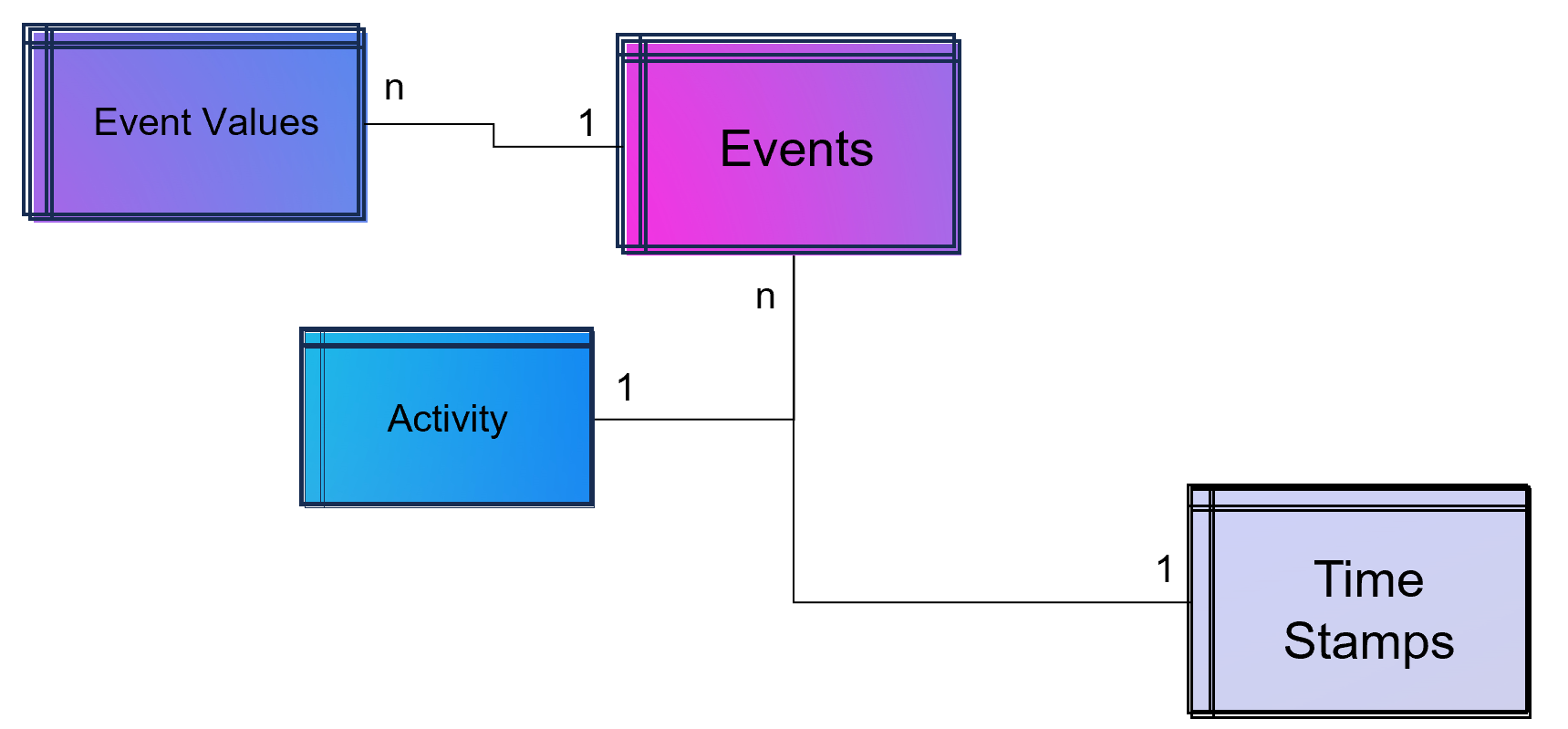
Cloud Data Platform for Shopfloor Management

How Cloud Data Platforms improve Shopfloor Management

In the era of Industry 4.0, linking data from MES (Manufacturing Execution System) with that from ERP, CRM and PLM systems plays an important role in creating integrated monitoring and control of business processes.

ERP (Enterprise Resource Planning) systems contain information about finance, supplier management, human resources and other operational processes, while CRM (Customer Relationship Management) systems provide data about customer relationships, marketing and sales activities. PLM (Product Lifecycle Management) systems contain information about products, development, design and engineering.

By linking this data with the data from MES, companies can obtain a more complete picture of their business operations and thus achieve better monitoring and control of their business processes. Of central importance here are the OEE (Overall Equipment Effectiveness) KPIs that are so important in production, as well as the key figures from financial controlling, such as contribution margins. The fusion of data in a central platform enables smooth analysis to optimize processes and increase business efficiency in the world of Industry 4.0 using methods from business intelligence, process mining and data science. Companies also significantly increase their enterprise value with the linking of this data, thanks to the data and information transparency gained.

Cloud Data Platform for shopfloor management and data sources such like MES, ERP, PLM and machine data.

Cloud Data Platform for shopfloor management and data sources such like MES, ERP, PLM and machine data. Copyright by DATANOMIQ.

If the data sources are additionally expanded to include the machines of production and logistics, much more in-depth analyses for error detection and prevention as well as for optimizing the factory in its dynamic environment become possible. The machine sensor data can be monitored directly in real time via respective data pipelines (real-time stream analytics) or brought into an overall picture of aggregated key figures (reporting). The readers of this data are not only people, but also individual machines or entire production plants that can react to this data.

As a central data architecture there are dozens of analytical applications which can be fed with data:

OEE key figures for Shopfloor reporting
Process Mining (e.g. material flow analysis) for manufacturing and supply chain.
Detection of anomalies on the shopfloor or on individual machines.
Predictive maintenance for individual machines or entire production lines.

This solution scales completely automatically in terms of both performance and cost. It looks beyond individual problems since it offers universal and flexible scope for action. In other words, it will result in a “god mode” for the management being able to drill-down from a specific client project to insights into single machines involved into each project.

Are you interested in scalable data architectures for your shopfloor management? Or would you like to discuss a specific problem with us? Or maybe you are interested in an individual data strategy? Then get in touch with me! 🙂

Data Dimensionality Reduction Series: Random Forest

Hello lovely individuals, I hope everyone is doing well, is fantastic, and is smiling more than usual. In this blog we shall discuss a very interesting term used to build many models in the Data science industry as well as the cyber security industry.

SUPER BASIC DEFINITION OF RANDOM FOREST:

Random forest is a form of Supervised Machine Learning Algorithm that operates on the majority rule. For example, if we have a number of different algorithms working on the same issue but producing different answers, the majority of the findings are taken into account. Random forests, also known as random selection forests, are an ensemble learning approach for classification, regression, and other problems that works by generating a jumble of decision trees during training.

When it comes to regression and classification, random forest can handle both categorical and continuous variable data sets. It typically helps us outperform other algorithms and overcome challenges like overfitting and the curse of dimensionality.

QUICK ANALOGY TO UNDERSTAND THINGS BETTER:

Uncle John wants to see a doctor for his acute abdominal discomfort, so he goes to his pals for recommendations on the top doctors in town. After consulting with a number of friends and family members, Atlas chooses to visit the doctor who received the highest recommendations.

So, what does this mean? The same is true for random forests. It builds decision trees from several samples and utilises their majority vote for classification and average for regression.

HOW BIAS AND VARIANCE AFFECTS THE ALGORITHM?

  1. BIAS
  • The algorithm’s accuracy or quality is measured.
  • High bias means a poor match
  1. VARIANCE
  • The accuracy or specificity of the match is measured.
  • A high variance means a weak match

We would like to minimise each of these. But, unfortunately we can’t do this independently, since there is a trade-off

EXPECTED PREDICTION ERROR = VARIANCE + BIAS^2 + NOISE^2

Bias vs Variance Tradeoff

HOW IS IT DIFFERENT FROM OTHER TWO ALGORITHMS?

Every other data dimensionality reduction method, such as missing value ratio and principal component analysis, must be built from the scratch, but the best thing about random forest is that it comes with built-in features and is a tree-based model that uses a combination of decision trees for non-linear data classification and regression.

Without wasting much time, let’s move to the main part where we’ll discuss the working of RANDOM FOREST:

WORKING WITH RANDOM FOREST:

As we saw in the analogy, RANDOM FOREST operates on the basis of ensemble technique; however, what precisely does ensemble technique mean? It’s actually rather straightforward. Ensemble simply refers to the combination of numerous models. As a result, rather than a single model, a group of models is utilised to create predictions.

ENSEMBLE TECHNIQUE HAS 2 METHODS:

Ensemble Learning: Bagging and Boosting

1] BAGGING

2] BOOSTING

Let’s dive deep to understand things better:

1] BAGGING:

LET’S UNDERSTAND IT THROUGH A BETTER VIEW:

Bagging simply helps us to reduce the variance in a loud datasets. It works on an ensemble technique.

  1. Algorithm independent : general purpose technique
  2. Well suited for high variance algorithms
  3. Variance reduction is achieved by averaging a group of data.
  4. Choose # of classifiers to build (B)

DIFFERENT TRAINING DATA:

  1. Sample Training Data with Replacement
  2. Same algorithm on different subsets of training data

APPLICATION :

  1. Use with high variance algorithms (DT, NN)
  2. Easy to parallelize
  3. Limitation: Loss of Interpretability
  4. Limitation: What if one of the features dominates?

SUMMING IT ALL UP:

  1. Ensemble approach = Bootstrap Aggregation.
  2. In bagging a random dataset is selected as shown in the above figure and then a model is built using those random data samples which is termed as bootstrapping.
  3. Now, when we train this random sample data it is not mendidate to select data points only once, while training the sample data we can select the individual data point more then once.
  4. Now each of these models is built and trained and results are obtained.
  5. Lastly the majority results are being considered.

We can even calculate  the error from this thing know as random forest OOB error:

RANDOM FORESTS: OOB ERROR  (Out-of-Bag Error) :

▪ From each bootstrapped sample, 1/3rd of it is kept aside as “Test”

▪ Tree built on remaining 2/3rd

▪ Average error from each of the “Test” samples is called “Out-of-Bag Error”

▪ OOB error provides a good estimate of model error

▪ No need for separate cross validation

2] BOOSTING:

Boosting in short helps us to improve our prediction by reducing error in predictive data analysis.

Weak Learner: only needs to generate a hypothesis with a training accuracy greater than 0.5, i.e., < 50% error over any distribution.

KEY INTUITION:

  1. Strong learners are very difficult to construct
  2. Constructing weaker Learners is relatively easy influence with the empirical squared improvement when assigned to the model

APPROACH OUTLINE:

  1. Start with a ML algorithm for finding the rough rules of thumb (a.k.a. “weak” or “base” algorithm)
  2. Call the base algorithm repeatedly, each time feeding it a different subset of the training examples
  3. The basic learning algorithm creates a new weak prediction rule each time it is invoked.
  4. After several rounds, the boosting algorithm must merge these weak rules into a single prediction rule that, hopefully, is considerably more accurate than any of the weak rules alone.

TWO KEY DETAILS :

  1. In each round, how is the distribution selected ?
  2. What is the best way to merge the weak rules into a single rule?

BOOSTING is classified into two types:

1] ADA BOOST

2] XG BOOST

As far as the Random forest is concerned it is said that it follows the bagging method, not a boosting method. As the name implies, boosting involves learning from others, which in turn increases learning. Random forests have trees that run in parallel. While creating the trees, there is no interaction between them.

Boosting helps us reduce the error by decreasing the bias whereas, on other hand, Bagging is a manner to decrease the variance within the prediction with the aid of generating additional information for schooling from the dataset using mixtures with repetitions to provide multi-sets of the original information.

How Bagging helps with variance – A Simple Example

BAGGED TREES

  1. Decision Trees have high variance
  2. The resultant tree (model) is determined by the training data.
  3. (Unpruned) Decision Trees tend to overfit
  4. One option: Cost Complexity Pruning

BAG TREES

  1. Sample with replacement (1 Training set → Multiple training sets)
  2. Train model on each bootstrapped training set
  3. Multiple trees; each different : A garden ☺
  4. Each DT predicts; Mean / Majority vote prediction
  5. Choose # of trees to build (B)

ADVANTAGES

Reduce model variance / instability.

RANDOM FOREST : VARIABLE IMPORTANCE

VARIABLE IMPORTANCE :

▪ Each time a tree is split due to a variable m, Gini impurity index of the parent node is higher than that of the child nodes

▪ Adding up all Gini index decreases due to variable m over all trees in the forest, gives a measure of variable importance

IMPORTANT FEATURES AND HYPERPARAMETERS:

  1. Diversity :
  2. Immunity to the curse of dimensionality :
  3. Parallelization :
  4. Train-Test split :
  5. Stability :
  6. Gini significance (or mean reduction impurity) :
  7. Mean Decrease Accuracy :

FEATURES THAT IMPROVE THE MODEL’S PREDICTIONS and SPEED :

  1. maximum_features :

Increasing max features often increases model performance since each node now has a greater number of alternatives to examine.

  1. n_estimators :

The number of trees you wish to create before calculating the maximum voting or prediction averages. A greater number of trees improves speed but slows down your code.

  1. min_sample_leaf :

If you’ve ever designed a decision tree, you’ll understand the significance of the minimal sample leaf size. A leaf is the decision tree’s last node. A smaller leaf increases the likelihood of the model collecting noise in train data.

  1. n_jobs :

This option instructs the engine on how many processors it is permitted to utilise.

  1. random_state :

This argument makes it simple to duplicate a solution. If given the same parameters and training data, a definite value of random state will always provide the same results.

  1. oob_score:

A random forest cross validation approach is used here. It is similar to the leave one out validation procedure, except it is significantly faster.

LET’S SEE THE STEPS INVOLVED IN IMPLEMENTATION OF RANDOM FOREST ALGORITHM:

Step1: Choose T- number of trees to grow

Step2: Choose m<p (p is the number of total features) —number of features used to calculate the best split at each node (typically 30% for regression, sqrt(p) for classification)

Step3: For each tree, choose a training set by choosing N times (N is the number of training examples) with replacement from the training set

Step4: For each node, calculate the best split, Fully grown and not pruned.

Step5: Use majority voting among all the trees

Following is a full case study and implementation of all the principles we just covered, in the form of a jupyter notebook including every concept and all you ever wanted to know about RANDOM FOREST.

GITHUB Repository for this blog article: https://gist.github.com/Vidhi1290/c9a6046f079fd5abafb7583d3689a410