Understanding Dropout and implementing it on MNIST dataset
Over-fitting is a major problem in deep learning and a plethora of techniques have been introduced to prevent it. One of the most effective one is called “dropout”. Let’s use the analogy of a person going to gym for understanding this. Let’s say the person going to gym mostly uses his dominant arm, say his right arm to pick up weights. After some time, he notices that his dominant arm is developing a large muscle, but not the other arm. So, what can he do? Obviously, he needs to involve both his arms while training. Sometimes he should stop using his right arm, and use the left arm to lift weights and vice versa.
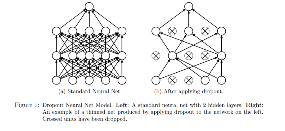
Something like this happens commonly in neural networks. Sometime one part of the network has very large weights and ends up dominating the training. While other part of the network remains weak and does not really play a role in the training. So, what dropout does to solve this problem, is it randomly shuts off some nodes and stop the gradients flowing through it. So, our forward and back propagation happen without those nodes. In that case the rest of the nodes need to pick up the slack and be more active in the training. We define a probability of the nodes getting dropped. For example, P=0.5 means there is a 50% chance a node will be dropped.
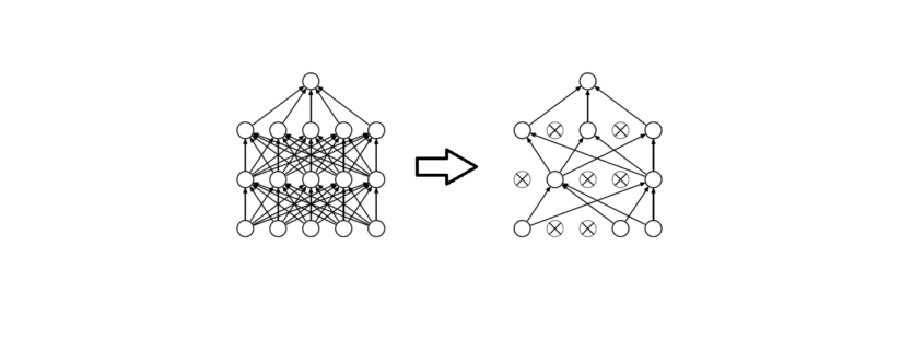
Figure 1 demonstrates the dropout technique, taken from the original research paper.
Our network can never rely on any given node because it can be squashed at any given time. Hence the network is forced to learn redundant representation for everything to make sure at least some of the information remains. Redundant representation leads our network to be more robust. It also acts as ensemble of many networks, since at every epoch random nodes are dropped, each time our network will be different. Ensemble of different networks perform better than a single network since they capture more randomness. Please note, only non-output nodes are dropped.
Let’s, look at the python code to implement dropout in a neural network:
|
1 2 3 4 5 6 7 8 9 10 11 12 13 14 15 16 17 18 19 20 21 22 23 24 25 26 27 28 29 30 31 32 33 34 35 36 37 38 39 40 41 42 43 44 45 46 47 48 49 50 51 52 53 54 55 56 57 58 59 60 61 62 63 64 65 66 67 68 69 70 71 72 73 74 75 76 77 78 79 80 81 82 83 84 85 86 87 88 89 90 91 92 93 94 95 96 97 98 99 100 101 102 103 104 105 106 107 108 109 110 |
from tensorflow.examples.tutorials.mnist import input_data mnist = input_data.read_data_sets(".", one_hot=True, reshape=False) import tensorflow as tf # Parameters learning_rate = 0.00001 epochs = 10 batch_size = 128 # Number of samples to calculate validation and accuracy test_valid_size = 256 # Network Parameters n_classes = 10 # MNIST total classes (0-9 digits) dropout = 0.75 # Dropout, probability to keep units # layers weight & bias weights = { 'wc1': tf.Variable(tf.random_normal([5, 5, 1, 32])), 'wc2': tf.Variable(tf.random_normal([5, 5, 32, 64])), 'wd1': tf.Variable(tf.random_normal([7*7*64, 1024])), 'out': tf.Variable(tf.random_normal([1024, n_classes]))} biases = { 'bc1': tf.Variable(tf.random_normal([32])), 'bc2': tf.Variable(tf.random_normal([64])), 'bd1': tf.Variable(tf.random_normal([1024])), 'out': tf.Variable(tf.random_normal([n_classes]))} #function that implements Convolution layer def conv2d(x, W, b, strides=1): x = tf.nn.conv2d(x, W, strides=[1, strides, strides, 1], padding='SAME') x = tf.nn.bias_add(x, b) return tf.nn.relu(x) #defining a function to implement maxpool layers def maxpool2d(x, k=2): return tf.nn.max_pool(x, ksize=[1, k, k, 1], strides=[1, k, k, 1], padding='SAME') #Function that defines all the convolution layers. def conv_net(x, weights, biases, dropout): # Layer 1 - 28*28*1 to 14*14*32 conv1 = conv2d(x, weights['wc1'], biases['bc1']) conv1 = maxpool2d(conv1, k=2) # Layer 2 - 14*14*32 to 7*7*64 conv2 = conv2d(conv1, weights['wc2'], biases['bc2']) conv2 = maxpool2d(conv2, k=2) # Fully connected layer - 7*7*64 to 1024 fc1 = tf.reshape(conv2, [-1, weights['wd1'].get_shape().as_list()[0]]) fc1 = tf.add(tf.matmul(fc1, weights['wd1']), biases['bd1']) fc1 = tf.nn.relu(fc1) fc1 = tf.nn.dropout(fc1, dropout) # Implementing the dropout layer # Output Layer - class prediction - 1024 to 10 out = tf.add(tf.matmul(fc1, weights['out']), biases['out']) return out # tf Graph input x = tf.placeholder(tf.float32, [None, 28, 28, 1]) y = tf.placeholder(tf.float32, [None, n_classes]) keep_prob = tf.placeholder(tf.float32) # Keep probability for dropout layers # Model logits = conv_net(x, weights, biases, keep_prob) # Define loss and optimizer cost = tf.reduce_mean(tf.nn.softmax_cross_entropy_with_logits(logits=logits, labels=y)) optimizer = tf.train.GradientDescentOptimizer(learning_rate=learning_rate).minimize(cost) # Accuracy correct_pred = tf.equal(tf.argmax(logits, 1), tf.argmax(y, 1)) accuracy = tf.reduce_mean(tf.cast(correct_pred, tf.float32)) # Initializing the variables init = tf.global_variables_initializer() # Launch the graph with tf.Session() as sess: sess.run(init) for epoch in range(epochs): for batch in range(mnist.train.num_examples//batch_size): batch_x, batch_y = mnist.train.next_batch(batch_size) sess.run(optimizer, feed_dict={x: batch_x, y: batch_y, keep_prob: dropout}) # Calculate batch loss and accuracy loss = sess.run(cost, feed_dict={x: batch_x, y: batch_y, keep_prob: 1.}) valid_acc = sess.run(accuracy, feed_dict={ x: mnist.validation.images[:test_valid_size], y: mnist.validation.labels[:test_valid_size], keep_prob: 1.}) #we want to keep all nodes while training so keep prob is 1. print('Epoch {:>2}, Batch {:>3} - Loss: {:>10.4f} Validation Accuracy: {:.6f}'.format( epoch + 1, batch + 1, loss, valid_acc)) # Calculate Test Accuracy test_acc = sess.run(accuracy, feed_dict={ x: mnist.test.images[:test_valid_size], y: mnist.test.labels[:test_valid_size], keep_prob: 1.}) print('Testing Accuracy: {}'.format(test_acc)) |


Leave a Reply
Want to join the discussion?Feel free to contribute!