On this paper discuss about CRISP-DM (Cross Industry Standard Process for data mining) methodology and its steps including selecting technique to successful the data mining process. Before going to CRISP-DM it is better to understand what data mining is? So, here first I introduce the data mining and then discuss about CRISP-DM and its steps for any beginner (data scientist) need to know.

1 Data Mining

Data mining is an exploratory analysis where has no idea about interesting outcome (Kantardzic, 2003). So data mining is a process to explore by analysis a large set of data to discover meaningful information which help the business to take a proper decision. For better business decision data mining is a way to select feature, correlation, and interesting patterns from large dataset (Fu, 1997; SPSS White Paper, 1999).

Data mining is a step by step process to discover knowledge from data. Pre-processing data is vital part for a data mining. In pre-process remove noisy data, combining multiple sources of data, retrieve relevant feature and transforming data for analysis. After pre-process mining algorithm applied to extract data pattern so data mining is a step by step process and applied algorithm to find meaning full data pattern. Actually data mining is not only conventional analysis it is more than that (Read, 1999).

Data mining and statistics closely related. Main goal of data mining and statistic is find the structure of data because data mining is a part of statistics (Hand, 1999). However, data mining use tools, techniques, database, machine learning which not part of statistics but data mining use statistics algorithm to find a pattern or discover hidden decision.

Data mining objective could be prediction or description. On prediction data mining considering several features of dataset to predict unidentified future, on the other hand description involve identifying pattern of data to interpreted (Kantardzic, 2003).

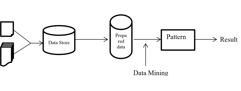
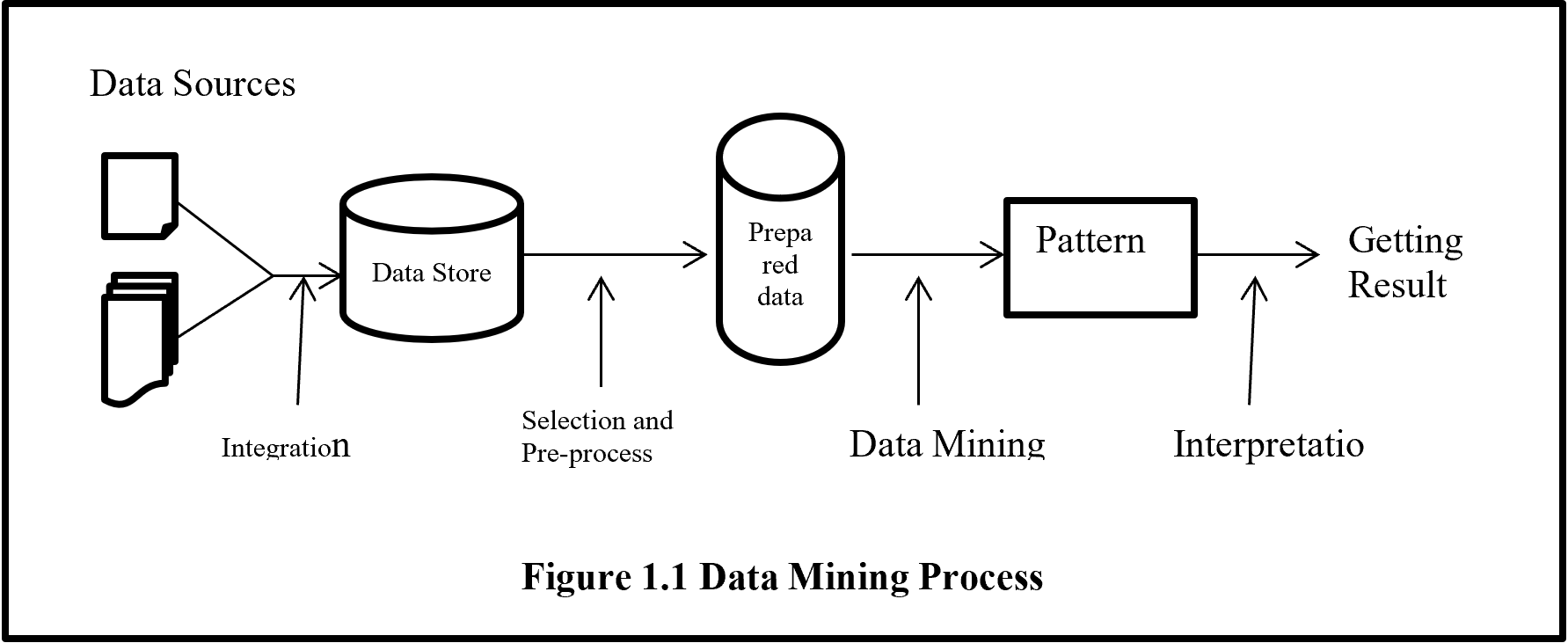
From figure 1.1 shows data mining is the only one part of getting unknown information from data but it is the central process of whole process. Before data mining there are several processes need to be done like collecting data from several sources than integrated data and keep in data storage. Stored unprocessed data evaluated and selected with pre-processed activity to give a standard format than data mining algorithm to analysis for hidden pattern.

2 CRISP-DM Methodologies

Cross Industry Standard Process for data mining (CRISP-DM) is most popular and widely uses data mining methodology. CRISP-DM breaks down the data mining project life cycle into six phases and each phase consists of many second-level generic tasks. Generic task cover all possible data mining application. CRISP-DM extends KDD (Knowledge Discovery and Data Mining) into six steps which are sequence of data mining application (Martínez-Plumed 2019).

Data science and data mining project extract meaningful information from data. Data science is an art where a lot of time need to spend for understanding the business value and data before applying any algorithm then evaluate and deployed a project. CRISP-DM help any data science and data mining project from start to end by giving step by step process.

Present world every day billions of data are generating. So organisations are struggling with overwhelmed data to process and find a business goal. Comprehensive data mining methodology, CRISP-DM help business to achieve desirable goal by analysing data.

CRISP-DM (Cross Industry Standard Process for Data Mining) is well documented, freely available, data mining methodology. CRISP-DM is developed by more than 200 data mining users and many mining tool and service providers funded by European Union. CRISP-DM encourages organization for best practice and provides a structure of data mining to get better, faster result.

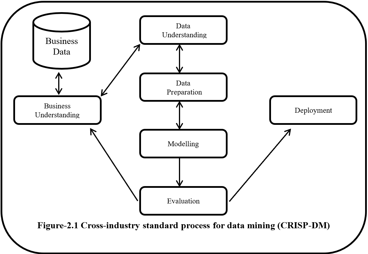
CRISP-DM is a step by step methodology. Figure-2.1 show the phases of CRISP-DM and process of data mining. Here one side arrow indicates the dependency between phases and double side arrow represents repeatable process. Six phases of CRISP-DM are Business understanding, Data understanding, Modelling, Evaluation and Deployment.

2.1 Business Understanding

Business Understanding or domain understanding is the first step of CRISP-DM methodology. On this stage identify the area of business which is going to transform into meaningful information by analysing, processing and implementing several algorithms. Business understanding identifies the available resource (human and hardware), problems and set a goal. Identification of business objective should be agreed with project sponsors and other unit of business which will be affected. This step also focuses about details business success criteria, requirements, constraints, risk, project plan and timeline.

2.2 Data Understanding

Data understanding is the second and closely related with the business understanding phase. This phase mainly focus on data collection and proceeds to get familiar with the data and also detect interesting subset from data. Data understanding has four subsets these are:-

2.2.1 Initial data collection

On this subset considering the data collection sources which is mainly divided into two categories like outsource data or internal source data.  If data is from outsource then it may costly, time consuming and may be low quality but if data is collected form internal source it is an easy and less costly, but it may be contain irrelevant data. If internal source data does not fulfil the interest of analysis than it is necessary to move outsource data. Data collection also give an assumption that the data is quantitative (continuous, count) or qualitative (categorical).  It also gives information about balance or imbalanced dataset.  On data collection should avoid random error, systematic error, exclusion errors, and errors of choosing.

2.2.2 Data Description

Data description performs initial analysis about data. On this stage it is going to determine about the source of data like RDBMS, SQL, NoSQL, Big data etc. then analysis and describe the data about size (large data set give more accurate result but time consuming), number of records, tables, database, variables, and data types (numeric, categorical or Boolean). On this phase examine the accessibility and availability of attributes.

2.2.3 Exploratory data analysis (EDA)

On exploratory data analysis describe the inferential statistics, descriptive statistics and graphical representation of data. Inferential statistics summarize the entire population from the sample data to perform sampling and hypothesis testing. On Parametric hypothesis testing  (Null or alternate – ANOVA, t-test, chi square test) perform for known distribution (based on population) like mean, variance, standard deviation, proportion and Non-parametric hypothesis testing perform when distribution is unknown or sample size is small. On sample dataset, random sampling implement when dataset is balance but for imbalance dataset should be follow random resampling (under  and over sampling), k fold cross validation, SMOTE (synthetic minority oversampling technique), cluster base sampling, ensemble techniques (bagging and boosting – Add boost, Gradient Tree Boosting, XG Boost) to form a balance dataset.

On descriptive statistics analysis describe about the mean, median, mode for measures of central tendency on first moment business decision. On second moment business decision describe the measure of dispersion about the variance, standard deviation and range of data.  On third and fourth moment business decision describe accordingly skewness (Positive skewness – heavier tail to the right, negative skewness – heavier tail to the left, Zero skewness – symmetric distribution) and Kurtosis (Leptokurtosis – heavy tail, platykurtosis – light tail, mesokurtic – normal distribution).

Graphical representation is divided into univariate, bivariate and multivariate analysis. Under univariate whisker plot, histogram identify the outliers and shape of distribution of data and Q-Q plot (Quantile – Quantile) plot describe the normality of data that means data is normally distribution or not.  On whisker plot if data present above of Q3 + 1.5 (IQR) and below of Q1 – 1.5 (IQR) is outlier. For Bivariate correlations identify with scatter plot which describe positive, negative or no correlation and also identify the data linearity or non-linearity. Scatter plot also describe the clusters and outliers of data.  For multivariate has no graphical analysis but used to use regression analysis, ANOVA, Hypothesis analysis.

2.2.4 Data Quality analysis

This phase identified and describes the potential errors like outliers, missing data, level of granularity, validation, reliability, bad metadata and inconsistency.  On this phase AAA (attribute agreement analysis) analysed discrete data for data error. Continuous data analysed with Gage repeatability and reproducibility (Gage R & R) which follow SOP (standard operating procedures). Here Gage R & R define the aggregation of variation in the measurement data because of the measurement system.

2.3 Data Preparation

Data Preparation is the time consuming stage for every data science project. Overall on every data science project 60% to 70% time spend on data preparation stage. Data preparation stapes are described below.

2.3.1 Data integration

Data integration involved to integrate or merged multiple dataset. Integration integrates data from different dataset where same attribute or same columns presents but when there is different attribute then merging the both dataset.

2.3.2 Data Wrangling

On this subset data are going to clean, curate and prepare for next level. Here analysis the outlier and treatment done with 3 R technique (Rectify, Remove, Retain) and for special cases if there are lots of outliner then need to treat outlier separately (upper outliner in an one dataset and lower outliner in another dataset) and alpha (significant value) trim technique use to separate the outliner from the original dataset. If dataset has a missing data then need to use imputation technique like mean, median, mode, regression, KNN etc.

If dataset is not normal or has a collinearity problem or autocorrelation then need to implement transformation techniques like log, exponential, sort, Reciprocal, Box-cox etc. On this subset use the data normalization (data –means/standard deviation) or standardization (min- max scaler) technique to make unitless and scale free data. This step also help if data required converting into categorical then need to use discretization or binning or grouping technique. For factor variable (where has limited set of values), dummy variable creation technique need to apply like one hot encoding.  On this subset also help heterogeneous data to transform into homogenous with clustering technique. Data inconsistencies also handle the inconsistence of data to make data in a single scale.

2.3.3 Feature engineering and selection/reduction

Feature engineering may called as attribute generation or feature extraction. Feature extraction creating new feature by reducing original feature to make simplex model. Feature engineering also do the normalized feature by producing calculative new feature. So feature engineering is a data pre-process technique where improve data quality by cleaning, integration, reduction, transformation and scaling.

Feature selections reduce the multicollinearity or high correlated data and make model simple. Main two type of feature selection technique are supervised and unsupervised. Principal Components Analysis (PCA) is an unsupervised feature reduction/ feature selection technique and LDA is a Linear Discriminant analysis supervised technique mainly use for classification problem. LDA analyse by comparing mean of the variables. Supervised technique is three types filter, wrapper and ensemble method. Filter method is easy to implement but wrapper is costly method and ensemble use inside a model.

2.4 Model

2.4.1 Model Selection Technique

Model selection techniques are influence by accuracy and performance.  Because recommendation need better performance but banking fraud detection needs better accuracy technique.  Model is mainly subdivided into two category supervised learning where predict an output variable according to given an input variable and unsupervised learning where has not output variable.

On supervised learning if an output variable is categorical than it is classification problem like two classes or multiclass classification problem. If an output variable is continuous (numerical) then the problem is called prediction problem. If need to recommending according to relevant information is called recommendation problem or if need to retrieve data according to relevance data is called retrieval problem.

On unsupervised learning where target or output variable is not present. On this technique all variable is treated as an input variable. Unsupervised learning also called clustering problem where clustering the dataset for future decision.

Reinforcement learning agent solves the problem by getting reward for success and penalty for any failure. And semi-supervised learning is a process to solve the problem by combining supervised and unsupervised learning method. On semi-supervised, a problem solved by apply unsupervised clustering technique then for each cluster apply different type of supervised machine learning algorithm like linear algorithm, neural network, K nearest  neighbour etc.

On data mining model selection technique, where output variable is known, then need to implement supervised learning.  Regression is the first choice where interpretation of parameter is important. If response variable is continuous then linear regression or if response variable is discrete with 2 categories value then logistic regression or if response variable is discrete with more than 2 categorical values then multinomial or ordinal regression or if response variable is count then poission where mean is equal to variance or negative binomial regression where variance is grater then mean or if response variable contain excessive zero values then need to choose Zero inflated poission (ZIP) or Zero inflated negative binomial (ZINB).

On supervised technique except regression technique all other technique can be used for both continuous or categorical response variable like KNN (K-Nearest Neighbour),  Naïve Bays, Black box techniques (Neural network, Support vector machine), Ensemble Techniques (Stacking, Bagging like random forest, Boosting like Decision tree, Gradient boosting, XGB, Adaboost).

When response variable is unknown then need to implement unsupervised learning. Unsupervised learning for row reduction is K-Means, Hierarchical etc., for columns reduction or dimension reduction PCA (principal component analysis), LDA (Linear Discriminant analysis), SVD (singular value decomposition) etc. On market basket analysis or association rules where measure are support and confidence then lift ration to determine which rules is important. There are recommendation systems, text analysis and NLP (Natural language processing) also unsupervised learning technique.

For time series need to select forecasting technique. Where forecasting may model based or data based. For Trend under model based need to use linear, exponential, quadratic techniques. And for seasonality need to use additive, multiplicative techniques. On data base approaches used auto regressive, moving average, last sample, exponential smoothing (e.g. SES – simple exponential smoothing, double exponential smoothing, and winters method).

2.4.2 Model building

After selection model according to model criterion model is need to be build. On model building provided data is subdivided with training, validation and testing.  But sometime data is subdivided just training and testing where information may leak from testing data to training data and cause an overfitting problem. So training dataset should be divided into training and validation whereas training model is tested with validation data and if need any tuning to do according to feedback from validation dataset. If accuracy is acceptable and error is reasonable then combine the training and validation data and build the model and test it on unknown testing dataset. If the training error and testing error is minimal or reasonable then the model is right fit or if the training error is low and testing error is high then model is over fitted (Variance) or if training error is high and testing error is also high then model is under fitted (bias). When model is over fitted then need to implement regularization technique (e.g. linear – lasso, ridge regression, Decision tree – pre-pruning, post-pruning, Knn – K value, Naïve Bays – Laplace, Neural network – dropout, drop connect, batch normalization, SVM –  kernel trick)

When data is balance then split the data training, validation and testing and here training is larger dataset then validation and testing. If data set is imbalance then need to use random resampling (over and under) by artificially increases training dataset. On random resampling by randomly partitioning data and for each partition implement the model and taking the average of accuracy. Under K fold cross validation creating K times cross dataset and creating model for every dataset and validate, after validation taking the average of accuracy of all model. There is more technique for imbalance dataset like SMOTH (synthetic minority oversampling technique), cluster based sampling, ensemble techniques e.g. Bagging, Boosting (Ada Boost, XGBoost).

2.4.3 Model evaluation and Tuning

On this stage model evaluate according to errors and accuracy and tune the error and accuracy for acceptable manner. For continuous outcome variable there are several way to measure the error like mean error, mean absolute deviation, Mean squared error, Root mean squared error, Mean percentage error and Mean absolute percentage error but more acceptable way is Mean absolute percentage error. For this continuous data if error is known then it is easy to find out the accuracy because accuracy and error combining value is one. The error function also called cost function or loss function.

For discrete output variable model, for evaluation and tuning need to use confusion matrix or cross table. From confusion matrix, by measuring accuracy, error, precision, sensitivity, specificity, F1 help to take decision about model fitness. ROC curve (Receiver operating characteristic curve), AUC curve (Area under the ROC curve) also evaluate the discrete output variable. AUC and ROC curve plot of sensitivity (true positive rate) vs 1-specificity (false positive rate).  Here sensitivity is a positive recall and  recall is basically out of all positive samples, how sample classifier able to identify. Specificity is negative recall here recall is out of all negative samples, how many sample classifier able to identify.  On AUC where more the area under the ROC is represent better accuracy. On ROC were step bend it’s indicate the cut off value.

2.4.4 Model Assessment

There is several ways to assess the model. First it is need to verify model performance and success according to desire achievement. It needs to identify the implemented model result according to accuracy where accuracy is repeatable and reproducible. It is also need to identify that the model is scalable, maintainable, robust and easy to deploy. On assessment identify that the model evaluation about satisfactory results (identify the precision, recall, sensitivity are balance) and meet business requirements.

2.5 Evaluation

On evaluation steps, all models which are built with same dataset, given a rank to find out the best model by assessing model quality of result and simplicity of algorithm and also cost of deployment. Evaluation part contains the data sufficiency report according to model result and also contain suggestion, feedback and recommendation from solutions team and SMEs (Subject matter experts) and record all these under OPA (organizational process assets).

2.6 Deployment

Deployment process needs to monitor under PEST (political economical social technological) changes within the organization and outside of the organization. PEST is similar to SWOT (strength weakness opportunity and thread) where SW represents the changes of internal and OT represents external changes.

On this deployment steps model should be seamless (like same environment, same result etc.) from development to production. Deployment plan contain the details of human resources, hardware, software requirements. Deployment plan also contain maintenance and monitoring plan by checking the model result and validity and if required then implement retire, replace and update plan.

3 Summaries

CRISP-DM implementation is costly and time consuming. But CRISP-DM methodology is an umbrella for data mining process. CRISP-DM has six phases, Business understanding, Data understanding, Modelling, Evaluation and Deployment. Every phase has several individual criteria, standard and process. CRISP-DM is Guideline for data mining process so if CRISP-DM is going to implement in any project it is necessary to follow each and every single guideline and maintain standard and criteria to get required result.

4 References

1. Fu, Y., (1997), “Data Mining: Tasks, Techniques and Applications”, Potentials, IEEE, 16: 4, 18–20.
2. Hand, D. J., (1999), “Statistics and Data Mining: Intersecting Disciplines”, ACM SIGKDD Explorations Newsletter, 1: 1, 16 – 19.
3. Kantardzic, M., (2003), “Data Mining: Concepts, Models, Methods, and Algorithms” John Wiley and Sons, Inc., Hoboken, New Jersey
4. Martínez-Plumed, F., Contreras-Ochando, L., Ferri, C., Orallo, J.H., Kull, M., Lachiche, N., Quintana, M.J.R. and Flach, P.A., 2019. CRISP-DM Twenty Years Later: From Data Mining Processes to Data Science Trajectories. IEEE Transactions on Knowledge and Data Engineering.
5. Read, B.J., (1999), “Data Mining and Science? Knowledge discovery in science as opposed to business”, 12th ERCIM Workshop on Database Research.