Tag Archive for: Predictive Analytics

Data Science and Predictive Analytics in Healthcare

Doing data science in a healthcare company can save lives. Whether it’s by predicting which patients have a tumor on an MRI, are at risk of re-admission, or have misclassified diagnoses in electronic medical records are all examples of how predictive models can lead to better health outcomes and improve the quality of life of patients.  Nevertheless, the healthcare industry presents many unique challenges and opportunities for data scientists.

The impact of data science in healthcare

Healthcare providers have a plethora of important but sensitive data. Medical records include a diverse set of data such as basic demographics, diagnosed illnesses, and a wealth of clinical information such as lab test results. For patients with chronic diseases, there could be a long and detailed history of data available on a number of health indicators due to the frequency of visits to a healthcare provider. Information from medical records can often be combined with outside data as well. For example, a patient’s address can be combined with other publicly available information to determine the number of surgeons that practice near a patient or other relevant information about the type of area that patients reside in.

With this rich data about a patient as well as their surroundings, models can be built and trained to predict many outcomes of interest. One important area of interest is models predicting disease progression, which can be used for disease management and planning. For example, at Fresenius Medical Care (where we primarily care for patients with chronic conditions such as kidney disease), we use a Chronic Kidney Disease progression model that can predict the trajectory of a patient’s condition to help clinicians decide whether and when to proceed to the next stage in their medical care. Predictive models can also notify clinicians about patients who may require interventions to reduce risk of negative outcomes. For instance, we use models to predict which patients are at risk for hospitalization or missing a dialysis treatment. These predictions, along with the key factors driving the prediction, are presented to clinicians who can decide if certain interventions might help reduce the patient’s risk.

Challenges of data science in healthcare

One challenge is that the healthcare industry is far behind other sectors in terms of adopting the latest technology and analytics tools. This does present some challenges, and data scientists should be aware that the data infrastructure and development environment at many healthcare companies will not be at the bleeding edge of the field. However it also means there are a lot of opportunities for improvement, and even small simple models can yield vast improvements over current methods.

Another challenge in the healthcare sector arises from the sensitive nature of medical information. Due to concerns over data privacy, it can often be difficult to obtain access to data that the company has. For this reason, data scientists considering a position at a healthcare company should be aware of whether there is already an established protocol for data professionals to get access to the data. If there isn’t, be aware that simply getting access to the data may be a major effort in itself.

Finally, it is important to keep in mind the end-use of any predictive model. In many cases, there are very different costs to false-negatives and false-positives. A false-negative may be detrimental to a patient’s health, while too many false-positives may lead to many costly and unnecessary treatments (also to the detriment of patients’ health for certain treatments as well as economy overall). Education about the proper use of predictive models and their limitations is essential for end-users. Finally, making sure the output of a predictive model is actionable is important. Predicting that a patient is at high-risk is only useful if the model outputs is interpretable enough to explain what factors are putting that patient at risk. Furthermore, if the model is being used to plan interventions, the factors that can be changed need to be highlighted in some way – telling a clinician that a patient is at risk because of their age is not useful if the point of the prediction is to lower risk through intervention.

The future of data science in the healthcare sector

The future holds a lot of promise for data science in healthcare. Wearable devices that track all kinds of activity and biometric data are becoming more sophisticated and more common. Streaming data coming from either wearables or devices providing treatment (such as dialysis machines) could eventually be used to provide real-time alerts to patients or clinicians about health events outside of the hospital.

Currently, a major issue facing medical providers is that patients’ data tends to exist in silos. There is little integration across electronic medical record systems (both between and within medical providers), which can lead to fragmented care. This can lead to clinicians receiving out of date or incomplete information about a patient, or to duplication of treatments. Through a major data engineering effort, these systems could (and should) be integrated. This would vastly increase the potential of data scientists and data engineers, who could then provide analytics services that took into account the whole patients’ history to provide a level of consistency across care providers. Data workers could use such an integrated record to alert clinicians to duplications of procedures or dangerous prescription drug combinations.

Data scientists have a lot to offer in the healthcare industry. The advances of machine learning and data science can and should be adopted in a space where the health of individuals can be improved. The opportunities for data scientists in this sector are nearly endless, and the potential for good is enormous.

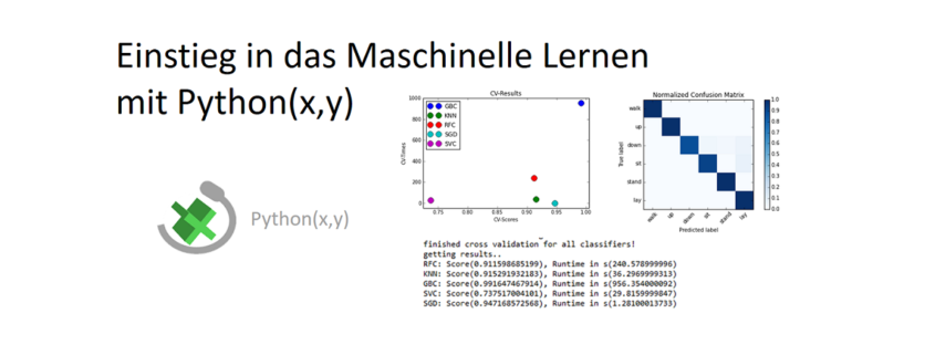
Einstieg in das Maschinelle Lernen mit Python(x,y)

Python(x,y) ist eine Python-Distribution, die speziell für wissenschaftliche Arbeiten entwickelt wurde. Es umfasst neben der Programmiersprache auch die Entwicklungsumgebung Spyder und eine Reihe integrierter Python-Bibliotheken. Mithilfe von Python(x,y) kann eine Vielzahl von Interessensbereichen bearbeitet werden. Dazu zählen unter anderem Bildverarbeitung oder auch das maschinelle Lernen. Das All-in-One-Setup für Python(x,y) ist für alle gängigen Betriebssysteme online erhältlich. Read more

Wahrscheinlichkeitsverteilungen – Zentralen Grenzwertsatz verstehen mit Pyhton

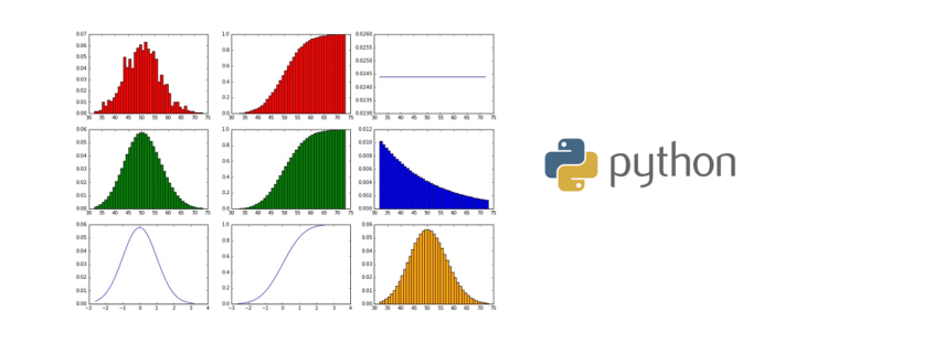
Wahrscheinlichkeitsverteilung sind im Data Science ein wichtiges Handwerkszeug. Während in der Mathevorlesung die Dynamik dieser Verteilungen nur durch wildes Tafelgekritzel schwierig erlebbar zu machen ist, können wir mit Programmierkenntnissen (in diesem Fall wieder mit Python) eine kleine Testumgebung für solche Verteilungen erstellen, um ein Gefühl dafür zu entwickeln, wie unterschiedlich diese auf verschiedene Wahrscheinlichkeitswerte, Varianz und Mengen an Datenpunkten reagieren und wann sie untereinander annäherungsweise ersetzbar sind – der zentrale Grenzwertsatz. Den Schwerpunkt lege ich in diesem Artikel auf die Binominal- und Normalverteilung.

Für die folgenden Beispiele werden folgende Python-Bibliotheken benötigt:

Read more

Neural Nets: Time Series Prediction

Artificial neural networks are very strong universal approximators. Google recently defeated the worlds strongest Go (“chinese chess”) player with two neural nets, which captured the game board as a picture. Aside from these classification tasks, neural nets can be used to predict future values, behaviors or patterns solely based on learned history. In the machine learning literature, this is often referred to as time series prediction, because, you know, values over time need to be predicted. Hah! To illustrate the concept, we will train a neural net to learn the shape of a sinusoidal wave, so it can continue to draw the shape without any help. We will do this with Scala. Scala is a great lang, because it is strongly typed but feels easy like Python. Throughout this article, I will use the library NeuroFlow, which is a simple, lightweight library I wrote to build and train nets. Because Open Source is the way to go, feel free to check (and contribute to? :-)) the code on GitHub.

Introduction of the shape

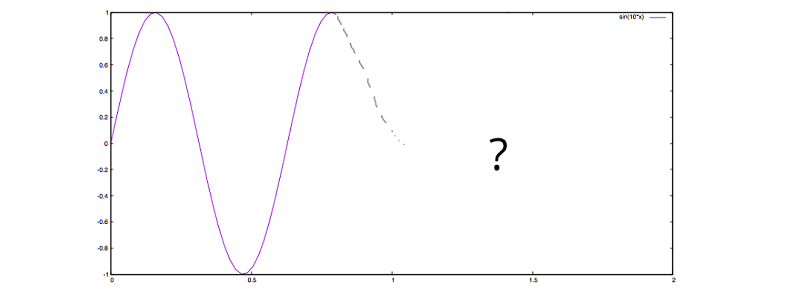
If we, as humans, want to predict the future based on historic observations, we would have no other chance but to be guided by the shape drawn so far. Let’s study the plot below, asking ourselves: How would a human continue the plot?

sinuspredictdr
f(x) = sin(10*x)

Intuitively, we would keep on oscillating up and down, just like the grey dotted line tries to rough out. To us, the continuation of the shape is reasonably easy to understand, but a machine does not have a gut feeling to ask for a good guess. However, we can summon a Frankenstein, which will be able to learn and continue the shape based on numbers. In order to do so, let’s have a look at the raw, discrete data of our sinusoidal wave:

x f(x)
0.0 0.0
0.05 0.479425538604203
0.10 0.8414709848078965
0.15 0.9974949866040544
0.20 0.9092974268256817
0.25 0.5984721441039564
0.30 0.1411200080598672
0.35 -0.35078322768961984
0.75 0.9379999767747389

Ranging from 0.0 until 0.75, these discrete values drawn from our function with step size 0.05 will be the basis for training. Now, one could come up with the idea to just memorize all values, so a sufficiently reasonable value can be picked based on comparison. For instance, to continue at the point 0.75 in our plot, we could simply examine the area close to 0.15, noticing a similar value close to 1, and hence go downwards. Well, of course this is cheating, but if a good cheat is a superior solution, why not cheat? Being hackers, we wouldn’t care. What’s really limiting here is the fact that the whole data set needs to be kept in memory, which can be infeasible for large sets, plus for more complex shapes, this approach would quickly result in a lot of weird rules and exceptions to be made in order to find comprehensible predictions.

Net to the rescue

Let’s go back to our table and see if a neural net can learn the shape, instead of simply memorizing it. Here, we want our net architecture to be of kind [3, 5, 3, 1]. Three input neurons, two hidden layers with five and three neurons respectively, as well as one neuron for the output layer will capture the data shown in the table.

sinuspredictnet

A supervised training mode means, that we want to train our net with three discrete steps as input and the fourth step as the supervised training element. So we will train a, b, c -> d and e, f, g -> h et cetera, hoping that this way our net will capture the slope pattern of our sinusoidal wave. Let’s code this in Scala:

First, we want a Tanh activation function, because the domain of our sinusoidal wave is [-1, 1], just like the hyperbolic tangent. This way we can be sure that we are not comparing apples with oranges. Further, we want a dynamic network (adaptive learning rate) and random initial weights. Let’s put this down:

No surprises here. After some experiments, we can pick values for the settings instance, which will promise good convergence during training. Now, let’s prepare our discrete steps drawn from the sinus function:

We will draw samples from the range with step size 0.05. After this, we will construct our training values xs as well as our supervised output values ys. Here, a group consists of 4 steps, with 3 steps as input and the last step as the supervised value.

After a pretty short time, we will see good news. Now, how can we check if our net can successfully predict the sinusoidal wave? We can’t simply call our net like a sinus function to map from one input value to one output value, e. g. something like net(0.75) == sin(0.75). Our net does not care about any x values, because it was trained purely based on the function values f(x), or the slope pattern in general. We need to feed our net with a three-dimensional input vector holding the first three, original function values to predict the fourth step, then drop the first original step and append the recently predicted step to predict the fifth step, et cetera. In other words, we need to traverse the net. Let’s code this:

with

So, basically we don’t just continue to draw the sinusoidal shape at the point 0.75, we draw the entire shape right from the start until 4.0 – solely based on our trained net! Now, let’s see how our Frankenstein will complete the sinusoidal shape from 0.75 on:

sinuspredictfintwo

I’d say, pretty neat? Keep in mind, here, the discrete predictions are connected through splines. Another interesting property of our trained net is its prediction compared to the original sinus function when taking the limit towards 4.0. Let’s plot both:

sinuspredictfin

The purple line is the original sinusoidal wave, whereas the green line is the prediction of our net. The first steps show great consistency, but slowly the curves diverge a little over time, as uncertainties will add up. To keep this divergence rather low, one could fine tune settings, for instance numeric precision. However, if one is taking the limit towards infinity, a perfect fit is illusory.

Final thoughts

That’s it! We have trained our net to learn and continue the sinusoidal shape. Now, I know that this is a rather academic example, but to train a neural net to learn more complex shapes is straightforward from here.

Thanks for reading!

Wahrscheinlichkeitesrechnung – Grundstein für Predictive Analytics

Die Wahrscheinlichkeitsrechnung behandelt die Gesetzmäßigkeiten  des (von außen betrachtet) zufälligen Vorkommens bestimmter Ereignisse aus einer vorgegebenen Ereignismenge. Die mathematische Statistik fasst diese Wahrscheinlichkeitsrechnung zur Stochastik zusammen, der Mathematik des Zufalls

Mit diesem Artikel – zu der ich eine Serie plane – möchte ich den Einstieg in Predictive Analytics wagen, zugegebenermaßen ein Themengebiet, in dem man sich sehr schnell verlieren und den Wald vor lauter Bäumen nicht mehr findet. Also belassen wir es erstmal bei einem sanften Einstieg…

Klassische Definition der Wahrscheinlichkeit

Das klassische Verständnis der Wahrscheinlichkeit geht von endlich vielen Ausgängen (Ereignisse) aus, bei denen alle Ausgänge gleich wahrscheinlich sind. Die dafür erdachten Zufallsexperimente wurden von dem französischen Mathematiker Pierre Simon Lapplace (1749 – 1827) zum ersten Mal nachvollziehbar beschrieben. Diese Zufallsexperimente werden daher auch Laplace-Experimente genannt.

Bei einem Laplace Experiment gilt:

Ereignismenge \Omega = {\omega_1,\omega_2,\omega_3,…\omega_s}
Wahrscheinlichkeit p(w_j)=\frac{1}{s}=\frac{1}{|\Omega|}
(j=1,2,3,…s)

Die Ergebnismenge, das ist die Menge aller möglichen Ereignisse, wird in der Regel mit einem \Omega (Omega) gekennzeichnet, ein beliebiges Einzelereignis hingegen als \omega (kleines Omega).

Eine typische Laplace-Wahrscheinlichkeitsfrage ist ein bevorstehender Würfelwurf. Wie groß ist die Wahrscheinlichkeit, mit einem echten (unverfälschten) Würfel eine gerade Zahl zu würfeln?

Mit \Omega={1,2,3,4,5,6} und A={2,4,6} folgt P(A)=\frac{|A|}{|\Omega|}=\frac{3}{6}=0,5.

Axiomatische Definition der Wahrscheinlichkeit

Jeder Wahrscheinlichkeitsbegriff muss auf denselben äußeren Bedingungen beruhenden Zufallsexperimenten beliebig oft wiederholbar sein. Die axiomatische Definition der Wahrscheinlichkeit P(A) eines Ereignisses A berücksichtigt Axiome. Axiome sind nicht beweisbare Grundpostulate, darunter fallen Gegebenheiten, die gewissermaßen unverstanden sind und deren Vorkommen und Bedeutung in der Regel empirisch belegt werden müssen.
Die Definition der axiomatischen Wahrscheinlichkeit stammt vom russischen Mathematiker Andrej Nikollajewitsch Kolmogorov (1903 – 1987).

In der Realität gibt es keine perfekte Zufälligkeit, denn jedes Ergebnis ist von ganz bestimmten Faktoren abhängig. Auf den Würfelwurf bezogen, hängt das gewürfelte Ergebnis von unüberschaubar vielen Faktoren ab. Wären diese alle bekannt, könnte das Ergebnis exakt berechnet und somit mit einer Sicherheit vorhergesagt werden. Da dafür jedoch in der Praxis unbestimmbar viele Faktoren eine Rolle spielen (beispielsweise die genaue Beschaffenheit des Würfels in Form, Gewicht, Materialwiderstand, der genaue Winkel, die Fallgeschwindigkeit, die Ausgangsposition der Hand und des Würfels) können wir das Ergebnis nur schätzen, indem die Beschreibung des Vorgangs vereinfacht wird. Nur diese Vereinfachung macht es uns möglich, Vorhersagen zu treffen, die dann jedoch nur eine Wahrscheinlichkeit darstellen und somit mit einer Unsicherheit verbunden sind.

In der abstrakten Welt des perfekten Zufalls gäbe es die gleiche Chance, eine “4” zu würfeln, wie jeweils alle anderen Ziffern.

Mit \Omega={1,2,3,4,5,6} und A={4} folgt P(A)=\frac{|A|}{|\Omega|}=\frac{1}{6}=0,167.

Das Ergebnis eines Wurfes des Würfels ist in der Realität auch von der Beschaffenheit des Würfels abhängig. Angenommen, der Würfel hat auf Seite der Ziffer “4” bei allen vier Kanten eine Abrundung, die ein Umkippen auf eine andere Seite begünstigen, so bedeutet dies:

  • Die Ziffer “4” hat vier abgerundete Kanten, die Wahrscheinlichkeit eine “4” zu würfeln sinkt stark
  • Die Ziffern “1”, “3”, “5”, “6” haben jeweils eine abgerundete Kante (Berühungskante zur “4”) sinkt
  • Die Ziffer “2” liegt der “4” gegenüber, hat somit keine Berührungskante und keine Abrundung, so steigt ihre Chance gewürfelt zu werden

Nun könnte sich nach einer empirischen Untersuchung mit einer ausreichenden Stichprobe folgende Wahrscheinlichkeit ergeben:

  • p(4) = 0,1
  • p(1) = p(3) = p(5) = p(6) = 0,15
  • p(2) = 0,3
  • P(\Omega) = 1,0

Durch die Analyse der bisherigen Wurf-Historie und der Betrachtung der Beschaffenheit der Kanten des Würfels können wir uns somit weit realistischere Wahrscheinlichkeiten über die Wurfergebnisse ermitteln. Wie hoch wäre nun die Wahrscheinlichkeit, nach einem Wurf eine gerade Zahl zu würfeln?

Mit \Omega={1,2,3,4,5,6} und A={2,4,6} folgt P(A)=p(2)+p(4)+p(6)=0,55.

Top 10 der Python Bibliotheken für Data Science

Python gilt unter Data Scientists als Alternative zu R Statistics. Ich bevorzuge Python auf Grund seiner Syntax und Einfachheit gegenüber R, komme hinsichtlich der vielen Module jedoch häufig etwas durcheinander. Aus diesem Grund liste ich hier die – meiner Einschätzung nach – zehn nützlichsten Bibliotheken für Python, um einfache Datenanalysen, aber auch semantische Textanalysen, Predictive Analytics und Machine Learning in die Tat umzusetzen.

NumPy – Numerische Analyse

NumPy ist eine Open Source Erweiterung für Python. Das Modul stellt vorkompilierte Funktionen für die numerische Analyse zur Verfügung. Insbesondere ermöglicht es den einfachen Umgang mit sehr großen, multidimensionalen Arrays (Listen) und Matrizen, bietet jedoch auch viele weitere grundlegende Features (z. B. Funktionen der Zufallszahlenbildung, Fourier Transformation, linearen Algebra). Ferner stellt das NumPy sehr viele Funktionen mathematische Funktionen für das Arbeiten mit den Arrays und Matrizen bereit.

matplotlib – 2D/3D Datenvisualisierung

Die matplotlib erweitert NumPy um grafische Darstellungsmöglichkeiten in 2D und 3D. Das Modul ist in Kombination mit NumPy wohl die am häufigsten eingesetzte Visualisierungsbibliothek für Python.

Die matplotlib bietet eine objektorientierte API, um die dynamischen Grafiken in Pyhton GUI-Toolkits einbinden zu können (z. B. GTL+ oder wxPython).

NumPy und matplotlib werden auch mit den nachfolgenden Bibliotheken kombiniert.

Bokeh – Interaktive Datenvisualisierung

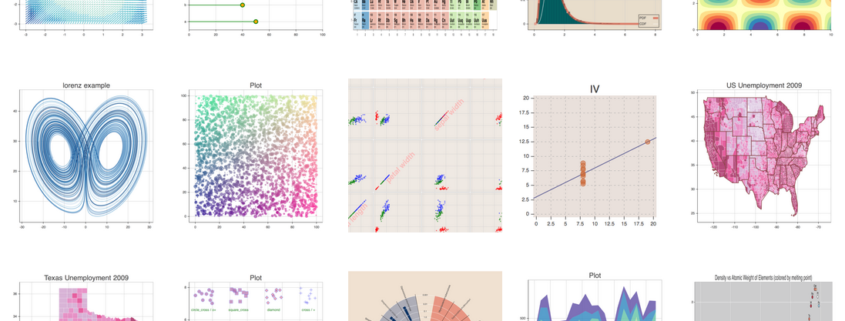
Während die Plot-Funktionen von matplotlib statisch angezeigt werden, kann in den Visualsierungsplots von Bokeh der Anwender interaktiv im Chart klicken und es verändern. Bokeh ist besonders dann geeignet, wenn die Datenvisualisierung als Dashboard im Webbrowser erfolgen soll.

Das Bild über diesen Artikel zeigt Visualiserungen mit dem Python Package Bokeh.

Pandas – Komplexe Datenanalyse

Pandas ist eine Bibliothek für die Datenverarbeitung und Datenanalyse mit Python. Es erweitert Python um Datenstrukturen und Funktionen zur Verarbeitung von Datentabellen. Eine besondere Stärke von Pandas ist die Zeitreihenanalyse. Pandas ist freie Software (BSD License).

Statsmodels – Statistische Datenanalyse

Statsmodels is a Python module that allows users to explore data, estimate statistical models, and perform statistical tests. An extensive list of descriptive statistics, statistical tests, plotting functions, and result statistics are available for different types of data and each estimator.

Die explorative Datenanalyse, statistische Modellierung und statistische Tests ermöglicht das Modul Statsmodels. Das Modul bringt neben vielen statistischen Funktionen auch eigene Plots (Visualisierungen) mit. Mit dem Modul wird Predictive Analytics möglich. Statsmodels wird häufig mit NumPy, matplotlib und Pandas kombiniert.

SciPy – Lineare Optimierung

SciPy ist ein sehr verbreitetes Mathematik-Modul für Python, welches den Schwerpunkt auf die mathematische Optimierung legt. Funktionen der linearen Algebra, Differenzialrechnung, Interpolation, Signal- und Bildverarbeitung sind in SciPy enthalten.

scikit-learn – Machine Learning

scikit-learn ist eine Framework für Python, das auf NumPy, matplotlob und SciPy aufsetzt, dieses jedoch um Funktionen für das maschinelle Lernen (Machine Learning) erweitert. Das Modul umfasst für das maschinelle Lernen notwendige Algorithmen für Klassifikationen, Regressionen, Clustering und Dimensionsreduktion.

Mlpy – Machine Learning

Alternativ zu scikit-learn, bietet auch Mlpy eine mächtige Bibliothek an Funktionen für Machine Learning. Mlpy setzt ebenfalls auf NumPy und SciPy, auf, erweitert den Funktionsumfang jedoch um Methoden des überwachten und unüberwachten maschinellen Lernens.

NLTK – Text Mining

NLTK steht für Natural Language Toolkit und ermöglicht den effektiven Einstieg ins Text Mining mit Python. Das Modul beinhaltet eigene (eher einfache) Visualisierungsmöglichkeiten zur Darstellung von Textmuster-Zusammenhängen, z. B. in Baumstrukturen. Für Text Mining und semantische Textanalysen mit Python gibt es wohl nichts besseres als NLTK.

Theano – Multidimensionale Berechnungen & GPU-Processing

Theano is a Python library that allows you to define, optimize, and evaluate mathematical expressions involving multi-dimensional arrays efficiently

Für multidimensionale Datenanalysen bzw. die Verarbeitung und Auswertung von multidimensionalen Arrays gibt es wohl nichts schnelleres als die Bibliothek Theano. Theano ist dabei eng mit NumPy verbunden.

Theano ermöglicht die Auslagerung der Berechnung auf die GPU (Grafikprozessor), was bis zu 140 mal schneller als auf der CPU sein soll. Getestet habe ich es zwar nicht, aber grundsätzlich ist es wahr, dass die GPU multidimensionale Arrays schneller verarbeiten kann, als die CPU. Zwar ist die CPU universeller (kann quasi alles berechnen), die GPU ist aber auf die Berechnung von 3D-Grafiken optimiert, die ebenfalls über multidimensionalen Vektoren verarbeitet werden.

DataQuest.io – Online Einstieg in Data Science mit Python

Data Science hat unglaublich viele Facetten und eine davon, ist die Analyse von Daten mit der Programmiersprache Python. Diese Programmiersprache ist neben R eine der am häufigsten eingesetzten Programmiersprachen für alle möglichen Aufgaben rund um die Auswertung von Daten.

Wer schon immer in die Datenanalyse mit Python einsteigen wollte, kann dies nun sehr einfach über einen ausgeklügelten Online-Kurs namens DataQuest tun.

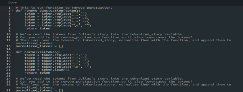
Ich selbst habe DataQuest ausprobiert und finde es super. Die ersten Module waren für mich erstmal sehr zäh, da sich diese mit Pythen und einigen Programmiergrundlagen befassen. Die Module können allerdings in beliebiger Reihenfolge abgearbeitet werden. Hat man den “Learning Python”-Teil aber durch, wird es schnell sehr spezifisch und auch als Experte kann die Aufgaben als guten Denksport verstehen.

Sehr gut dabei ist, dass der komplette Kurs online in der Cloud stattfindet. Benötigt wird nichts weiter als ein gewöhnlicher Internet-Browser und man muss sich nicht mit der Einrichtung von Python und der Entwicklungsumgebung auf dem Computer beschäftigen. DataQuest stellt über den Browser server-seitig die Entwicklungsumgebung bereit. Es kann also sofort nach der Account-Einrichtung losgehen! Die Kurse von DataQuest gibt es allerdings nur auf Englisch.

Der Kursumfang beginnt recht ausführlich über die Grundlagen der Programmierung, basierend auf Python. Die Grundlagen werden jedoch bereits überwiegend anhand von Aufgaben im Bereich der Datenanalyse erklärt, beispielsweise den Zugriff auf Textdateien.

Zumindest alle Grundlagen-Kurse sind kostenlos. Der weitere Kursinhalt über die Programmiergrundlagen hinaus befasst sich direkt mit dem Einstieg in Data Science mit der explorativen Datenanalyse, der Datenvisualisierung und der Statistik im Allgemeinen und Predictive Analytics im Speziellen. Ferner sollen in der Zukunft Kurse mit einen Einstieg ins Maschinelle Lernen (Machine Learning) angeboten werden. Die interessantesten Kurse können jedoch nur über den Premium-Account gestartet werden. Dieser ist für bezahlbare 35 US-Dollar pro Monat zu haben.

URL zum Anbieter: www.dataquest.io