Linear Algebra Archives

Tag Archive for: Linear Algebra

Understanding Linear Regression with all Statistical Terms

May 2, 2022/in Data Science, Main Category/by M.Nithya Lakshmi

Linear Regression Model – This article is about understanding the linear regression with all the statistical terms.

What is Regression Analysis?

regression is an attempt to determine the relationship between one dependent and a series of other independent variables.

Regression analysis is a form of predictive modelling technique which investigates the relationship between a dependent (target) and independent variable (s) (predictor). This technique is used for forecasting, time series modelling and finding the causal effect relationship between the variables. For example, relationship between rash driving and number of road accidents by a driver is best studied through regression.

Why do we use Regression Analysis?

As mentioned above, regression analysis estimates the relationship between two or more variables. Let’s understand this with an easy example:

Let’s say, you want to estimate growth in sales of a company based on current economic conditions. You have the recent company data which indicates that the growth in sales is around two and a half times the growth in the economy. Using this insight, we can predict future sales of the company based on current & past information.

There are multiple benefits of using regression analysis. They are as follows:

It indicates the significant relationships between dependent variable and independent variable. It indicates the strength of impact of multiple independent variables on a dependent variable. Regression analysis also allows us to compare the effects of variables measured on different scales, such as the effect of price changes and the number of promotional activities. These benefits help market researchers / data analysts / data scientists to eliminate and evaluate the best set of variables to be used for building predictive models.

There are various kinds of regression techniques available to make predictions. These techniques are mostly driven by three metrics (number of independent variables, type of dependent variables and shape of regression line).

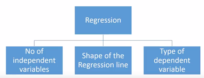
Number of independent variables, shape of regression line and type of dependent variable.

What is Linear Regression?

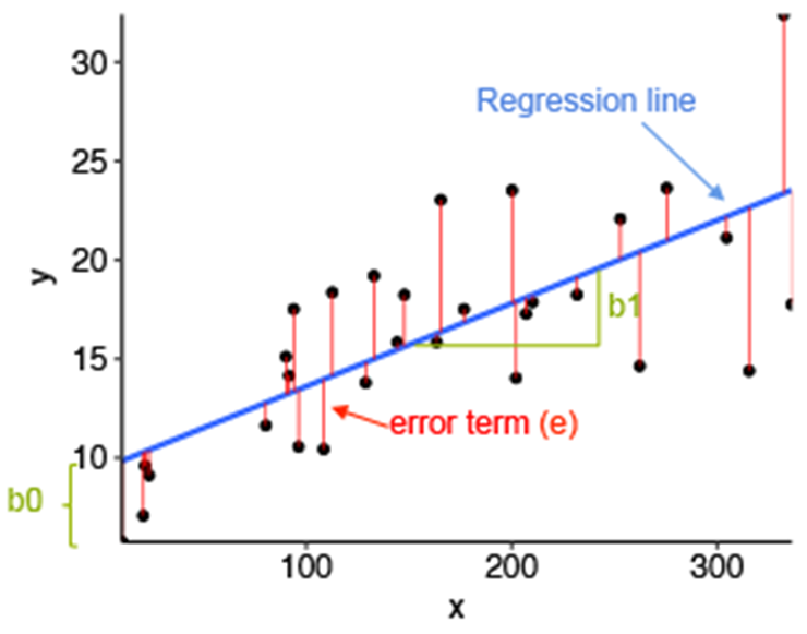
Linear Regression is the supervised Machine Learning model in which the model finds the best fit linear line between the independent and dependent variable i.e it finds the linear relationship between the dependent and independent variable.

Equation of Simple Linear Regression, where bo is the intercept, b1 is coefficient or slope, x is the independent variable and y is the dependent variable.

Equation of Multiple Linear Regression, where bo is the intercept, b1,b2,b3,b4…,bn are coefficients or slopes of the independent variables x1,x2,x3,x4…,xn and y is the $y=b_0+b_1x_1+b_2x_2+…+b_nx_n$ dependent variable.

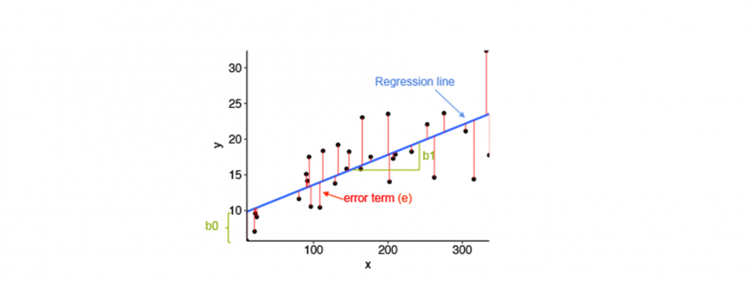
Linear regression and its error termin per value

Mathematical Approach:

Residual/Error = Actual values – Predicted Values
Sum of Residuals/Errors = Sum(Actual- Predicted Values)
Square of Sum of Residuals/Errors = (Sum(Actual- Predicted Values))^2

$\sum(e_i^2)=\sum(y_i-\hat{y_i})^2$

Application of Linear Regression:

Real-world examples of linear regression models

Businesses often use linear regression to understand the relationship between advertising spending and revenue.
Medical researchers often use linear regression to understand the relationship between drug dosage and blood pressure of patients.
Agricultural scientists often use linear regression to measure the effect of fertilizer and water on crop yields.
Data scientists for professional sports teams often use linear regression to measure the effect that different training regimens have on player performance.
Stock predictions: A lot of businesses use linear regression models to predict how stocks will perform in the future. This is done by analyzing past data on stock prices and trends to identify patterns.
Predicting consumer behavior: Businesses can use linear regression to predict things like how much a customer is likely to spend. Regression models can also be used to predict consumer behavior. This can be helpful for things like targeted marketing and product development. For example, Walmart uses linear regression to predict what products will be popular in different regions of the country.

Assumptions of Linear Regression:

Linearity: It states that the dependent variable Y should be linearly related to independent variables. This assumption can be checked by plotting a scatter plot between both variables.

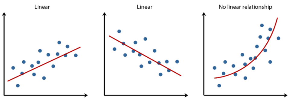
Normality: The X and Y variables should be normally distributed. Histograms, KDE plots, Q-Q plots can be used to check the Normality assumption.

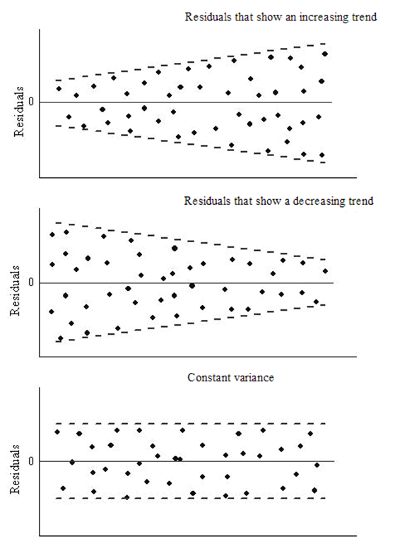
Homoscedasticity: The variance of the error terms should be constant i.e the spread of residuals should be constant for all values of X. This assumption can be checked by plotting a residual plot. If the assumption is violated then the points will form a funnel shape otherwise they will be constant.

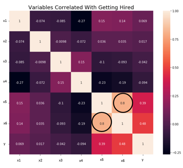
Independence/No Multicollinearity: The variables should be independent of each other i.e no correlation should be there between the independent variables. To check the assumption, we can use a correlation matrix or VIF score. If the VIF score is greater than 5 then the variables are highly correlated.

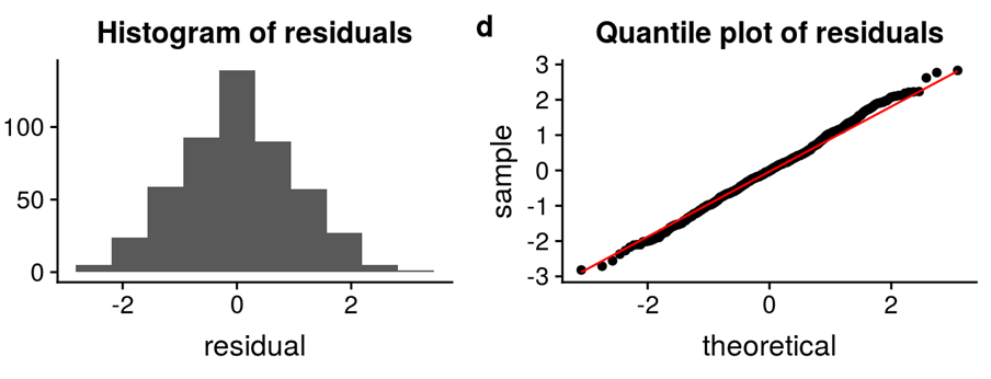
The error terms should be normally distributed. Q-Q plots and Histograms can be used to check the distribution of error terms.

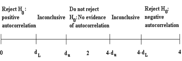
No Autocorrelation: The error terms should be independent of each other. Autocorrelation can be tested using the Durbin Watson test. The null hypothesis assumes that there is no autocorrelation. The value of the test lies between 0 to 4. If the value of the test is 2 then there is no autocorrelation.

Rethinking linear algebra part two: ellipsoids in data science

June 6, 2021/in Artificial Intelligence, Data Mining, Data Science, Data Science Hack, Machine Learning, Main Category, Python, Tutorial/by Yasuto Tamura

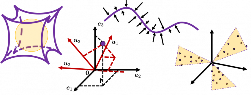
*This is the fourth article of my article series “Illustrative introductions on dimension reduction.”

1 Our expedition of eigenvectors still continues

This article is still going to be about eigenvectors and PCA, and this article still will not cover LDA (linear discriminant analysis). Hereby I would like you to have more organic links of the data science ideas with eigenvectors.

In the second article, we have covered the following points:

You can visualize linear transformations with matrices by calculating displacement vectors, and they usually look like vectors swirling.
Diagonalization is finding a direction in which the displacement vectors do not swirl, and that is equal to finding new axis/basis where you can describe its linear transformations more straightforwardly. But we have to consider diagonalizability of the matrices.
In linear dimension reduction such as PCA or LDA, we mainly use types of matrices called positive definite or positive semidefinite matrices.

In the last article we have seen the following points:

PCA is an algorithm of calculating orthogonal axes along which data “swell” the most.
PCA is equivalent to calculating a new orthonormal basis for the data where the covariance between components is zero.
You can reduced the dimension of the data in the new coordinate system by ignoring the axes corresponding to small eigenvalues.
Covariance matrices enable linear transformation of rotation and expansion and contraction of vectors.

I emphasized that the axes are more important than the surface of the high dimensional ellipsoids, but in this article let’s focus more on the surface of ellipsoids, or I would rather say general quadratic curves. After also seeing how to draw ellipsoids on data, you would see the following points about PCA or eigenvectors.

Covariance matrices are real symmetric matrices, and also they are positive semidefinite. That means you can always diagonalize covariance matrices, and their eigenvalues are all equal or greater than 0.
PCA is equivalent to finding axes of quadratic curves in which gradients are biggest. The values of quadratic curves increases the most in those directions, and that means the directions describe great deal of information of data distribution.
Intuitively dimension reduction by PCA is equal to fitting a high dimensional ellipsoid on data and cutting off the axes corresponding to small eigenvalues.

Even if you already understand PCA to some extent, I hope this article provides you with deeper insight into PCA, and at least after reading this article, I think you would be more or less able to visually control eigenvectors and ellipsoids with the Numpy and Maplotlib libraries.

*Let me first introduce some mathematical facts and how I denote them throughout this article in advance. If you are allergic to mathematics, take it easy or please go back to my former articles.

Any quadratic curves can be denoted as $\boldsymbol{x}^T A\boldsymbol{x} + 2\boldsymbol{b}^T\boldsymbol{x} + s = 0$ , where $\boldsymbol{x}\in \mathbb{R}^D$ $, A \in \mathbb{R}^{D\times D}$ $\boldsymbol{b}\in \mathbb{R}^D$ $s\in \mathbb{R}$ .
When I want to clarify dimensions of variables of quadratic curves, I denote parameters as $A_D, b_D$ .
If a matrix $A$ is a real symmetric matrix, there exist a rotation matrix $U$ such that $U^T A U = \Lambda$ , where $\Lambda = diag(\lambda_1, \dots, \lambda_D)$ and $U = (\boldsymbol{u}_1, \dots , \boldsymbol{u}_D)$ . $\boldsymbol{u}_1, \dots , \boldsymbol{u}_D$ are eigenvectors corresponding to $\lambda_1, \dots, \lambda_D$ respectively.
PCA corresponds to a case of diagonalizing $A$ where $A$ is a covariance matrix of certain data. When I want to clarify that $A$ is a covariance matrix, I denote it as $A=\Sigma$ .
Importantly covariance matrices $\Sigma$ are positive semidefinite and real symmetric, which means you can always diagonalize $\Sigma$ and any of their engenvalues cannot be lower than 0.

*In the last article, I denoted the covariance of data as $S$ , based on Pattern Recognition and Machine Learning by C. M. Bishop.

*Sooner or later you are going to see that I am explaining basically the same ideas from different points of view, using the topic of PCA. However I believe they are all important when you learn linear algebra for data science of machine learning. Even you have not learnt linear algebra or if you have to teach linear algebra, I recommend you to first take a review on the idea of diagonalization, like the second article. And you should be conscious that, in the context of machine learning or data science, only a very limited type of matrices are important, which I have been explaining throughout this article.

2 Rotation or projection?

In this section I am going to talk about basic stuff found in most textbooks on linear algebra. In the last article, I mentioned that if $A$ is a real symmetric matrix, you can diagonalize $A$ with a rotation matrix $U = (\boldsymbol{u}_1 \: \cdots \: \boldsymbol{u}_D)$ , such that $U^{-1}AU$ $= U^{T}AU$ $=\Lambda$ , where $\Lambda = diag(\lambda_{1}, \dots , \lambda_{D})$ . I also explained that PCA is a case where $A=\Sigma$ , that is, $A$ is the covariance matrix of certain data. $\Sigma$ is known to be positive semidefinite and real symmetric. Thus you can always diagonalize $\Sigma$ and any of their engenvalues cannot be lower than 0.

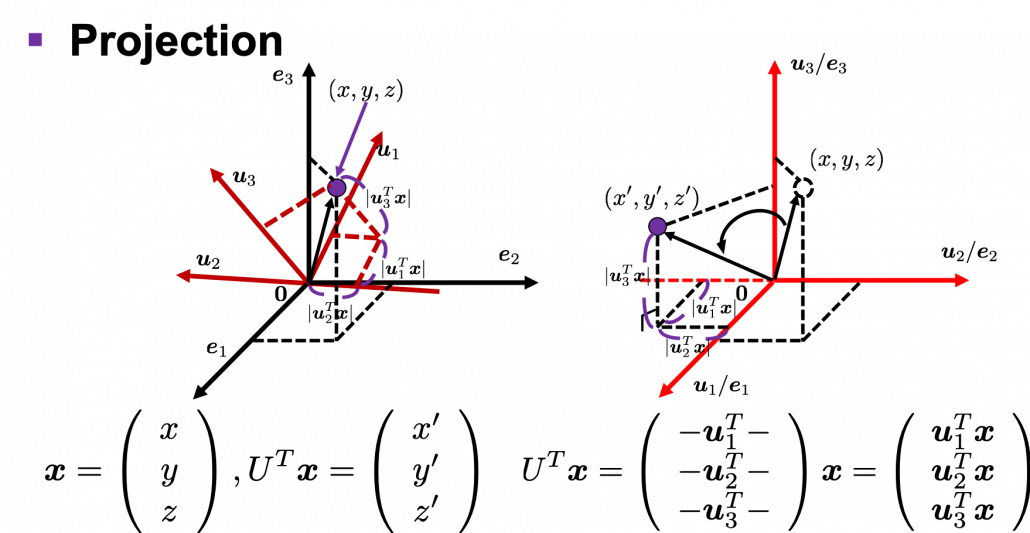
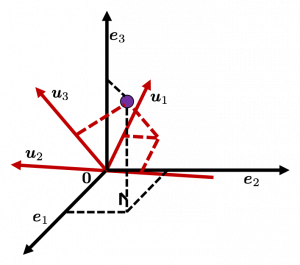
I think we first need to clarify the difference of rotation and projection. In order to visualize the ideas, let’s consider a case of $D=3$ . Assume that you have got an orthonormal rotation matrix $U = (\boldsymbol{u}_1 \: \boldsymbol{u}_2 \: \boldsymbol{u}_3)$ which diagonalizes $A$ . In the last article I said diagonalization is equivalent to finding new orthogonal axes formed by eigenvectors, and in the case of this section you got new orthonoramal basis $(\boldsymbol{u}_1, \boldsymbol{u}_2, \boldsymbol{u}_3)$ which are in red in the figure below. Projecting a point $\boldsymbol{x} = (x, y, z)$ on the new orthonormal basis is simple: you just have to multiply $\boldsymbol{x}$ with $U^T$ . Let $U^T \boldsymbol{x}$ be $(x', y', z')^T$ , and then $\left( \begin{array}{c} x' \\ y' \\ z' \end{array} \right) = U^T\boldsymbol{x} = \left( \begin{array}{c} \boldsymbol{u}_1^{T}\boldsymbol{x} \\ \boldsymbol{u}_2^{T}\boldsymbol{x} \\ \boldsymbol{u}_3^{T}\boldsymbol{x} \end{array} \right)$ . You can see $x', y', z'$ are $\boldsymbol{x}$ projected on $\boldsymbol{u}_1, \boldsymbol{u}_2, \boldsymbol{u}_3$ respectively, and the left side of the figure below shows the idea. When you replace the orginal orthonormal basis $(\boldsymbol{e}_1, \boldsymbol{e}_2, \boldsymbol{e}_3)$ with $(\boldsymbol{u}_1, \boldsymbol{u}_2, \boldsymbol{u}_3)$ as in the right side of the figure below, you can comprehend the projection as a rotation from $(x, y, z)$ to $(x', y', z')$ by a rotation matrix $U^T$ .

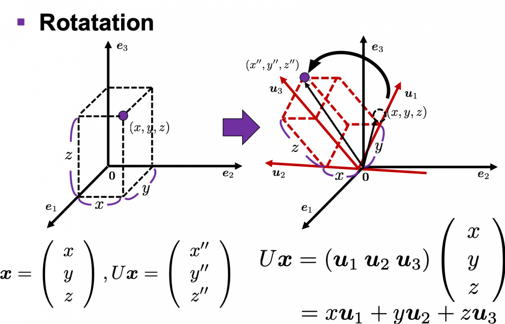
Next, let’s see what rotation is. In case of rotation, you should imagine that you rotate the point $\boldsymbol{x}$ in the same coordinate system, rather than projecting to other coordinate system. You can rotate $\boldsymbol{x}$ by multiplying it with $U$ . This rotation looks like the figure below.

In the initial position, the edges of the cube are aligned with the three orthogonal black axes $(\boldsymbol{e}_1, \boldsymbol{e}_2 , \boldsymbol{e}_3)$ , with one corner of the cube located at the origin point of those axes. The purple dot denotes the corner of the cube directly opposite the origin corner. The cube is rotated in three dimensions, with the origin corner staying fixed in place. After the rotation with a pivot at the origin, the edges of the cube are now aligned with a new set of orthogonal axes $(\boldsymbol{u}_1, \boldsymbol{u}_2 , \boldsymbol{u}_3)$ , shown in red. You might understand that more clearly with an equation: $U\boldsymbol{x} = (\boldsymbol{u}_1 \: \boldsymbol{u}_2 \: \boldsymbol{u}_3) \left( \begin{array}{c} x \\ y \\ z \end{array} \right)$ $= x\boldsymbol{u}_1 + y\boldsymbol{u}_2 + z\boldsymbol{u}_3$ . In short this rotation means you keep relative position of $\boldsymbol{x}$ , I mean its coordinates $(x, y, z)$ , in the new orthonormal basis. In this article, let me call this a “cube rotation.”

The discussion above can be generalized to spaces with dimensions higher than 3. When $U \in \mathbb{R}^{D \times D}$ is an orthonormal matrix and a vector $\boldsymbol{x} \in \mathbb{R}^D$ , you can project $\boldsymbol{x}$ to $\boldsymbol{x}' = U^T \boldsymbol{x}$ or rotate it to $\boldsymbol{x}'' = U \boldsymbol{x}$ , where $\boldsymbol{x}' = (x_{1}', \dots, x_{D}')^T$ and $\boldsymbol{x}'' = (x_{1}'', \dots, x_{D}'')^T$ . In other words $\boldsymbol{x} = U \boldsymbol{x}'$ , which means you can rotate back $\boldsymbol{x}'$ to the original point $\boldsymbol{x}$ with the rotation matrix $U$ .

I think you at least saw that rotation and projection are basically the same, and that is only a matter of how you look at the coordinate systems. But I would say the idea of projection is more important through out this article.

Let’s consider a function $f(\boldsymbol{x}; A) = \boldsymbol{x}^T A \boldsymbol{x} = (\boldsymbol{x}, A \boldsymbol{x})$ , where $A\in \mathbb{R}^{D\times D}$ is a real symmetric matrix. The distribution of $f(\boldsymbol{x}; A)$ is quadratic curves whose center point covers the origin, and it is known that you can express this distribution in a much simpler way using eigenvectors. When you project this function on eigenvectors of $A$ , that is when you substitute $U \boldsymbol{x}'$ for $\boldsymbol{x}$ , you get $f = (\boldsymbol{x}, A \boldsymbol{x})$ $=(U \boldsymbol{x}', AU \boldsymbol{x}')$ $= (\boldsymbol{x}')^T U^TAU \boldsymbol{x}'$ $= (\boldsymbol{x}')^T \Lambda \boldsymbol{x}'$ $= \lambda_1 ({x'}_1)^2 + \cdots + \lambda_D ({x'}_D)^2$ . You can always diagonalize real symmetric matrices, so the formula implies that the shapes of quadratic curves largely depend on eigenvectors. We are going to see this in detail in the next section.

* $(\boldsymbol{x}, \boldsymbol{y})$ denotes an inner product of $\boldsymbol{x}$ and $\boldsymbol{y}$ .

*We are going to see details of the shapes of quadratic “curves” or “functions” in the next section.

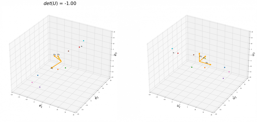
To be exact, you cannot naively multiply $U$ or $U^T$ for rotation. Let’s take a part of data I showed in the last article as an example. In the figure below, I projected data on the basis $(\boldsymbol{u}_1, \boldsymbol{u}_2 , \boldsymbol{u}_3)$ .

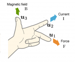
You might have noticed that you cannot do a “cube rotation” in this case. If you make the coordinate system $(\boldsymbol{u}_1, \boldsymbol{u}_2, \boldsymbol{u}_3)$ with your left hand, like you might have done in science classes in school to learn Fleming’s rule, you would soon realize that the coordinate systems in the figure above do not match. You need to flip the direction of one axis to match them.

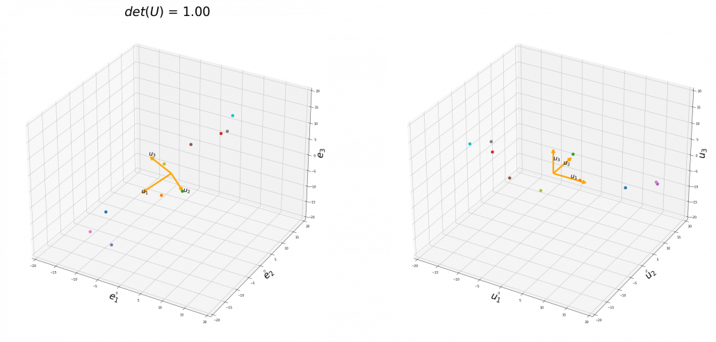
Mathematically, you have to consider the determinant of the rotation matrix $U$ . You can do a “cube rotation” when $det(U)=1$ , and in the case above $det(U)$ was $-1$ , and you needed to flip one axis to make the determinant $1$ . In the example in the figure below, you can match the basis. This also can be generalized to higher dimensions, but that is also beyond the scope of this article series. If you are really interested, you should prepare some coffee and snacks and textbooks on linear algebra, and some weekends.

When you want to make general ellipsoids in a 3d space on Matplotlib, you can take advantage of rotation matrices. You first make a simple ellipsoid symmetric about xyz axis using polar coordinates, and you can rotate the whole ellipsoid with rotation matrices. I made some simple modules for drawing ellipsoid. If you put in a rotation matrix which diagonalize the covariance matrix of data and a list of three radiuses $\sqrt{\lambda_1}, \sqrt{\lambda_2}, \sqrt{\lambda_3}$ , you can rotate the original ellipsoid so that it fits the data well.

3 Types of quadratic curves.

*This article might look like a mathematical writing, but I would say this is more about computer science. Please tolerate some inaccuracy in terms of mathematics. I gave priority to visualizing necessary mathematical ideas in my article series. If you are not sure about details, please let me know.

In linear dimension reduction, or at least in this article series you mainly have to consider ellipsoids. However ellipsoids are just one type of quadratic curves. In the last article, I mentioned that when the center of a D dimensional ellipsoid is the origin point of a normal coordinate system, the formula of the surface of the ellipsoid is as follows: $(\boldsymbol{x}, A\boldsymbol{x})=1$ , where $A$ satisfies certain conditions. To be concrete, when $(\boldsymbol{x}, A\boldsymbol{x})=1$ is the surface of a ellipsoid, $A$ has to be diagonalizable and positive definite.

*Real symmetric matrices are diagonalizable, and positive definite matrices have only positive eigenvalues. Covariance matrices $\Sigma$ , whose displacement vectors I visualized in the last two articles, are known to be symmetric real matrices and positive semi-defintie. However, the surface of an ellipsoid which fit the data is $\boldsymbol{x}^T \Sigma ^{-1} \boldsymbol{x} = const.$ , not $\boldsymbol{x}^T \Sigma \boldsymbol{x} = const.$ .

*You have to keep it in mind that $\boldsymbol{x}$ are all deviations.

*You do not have to think too much about what the “semi” of the term “positive semi-definite” means fow now.

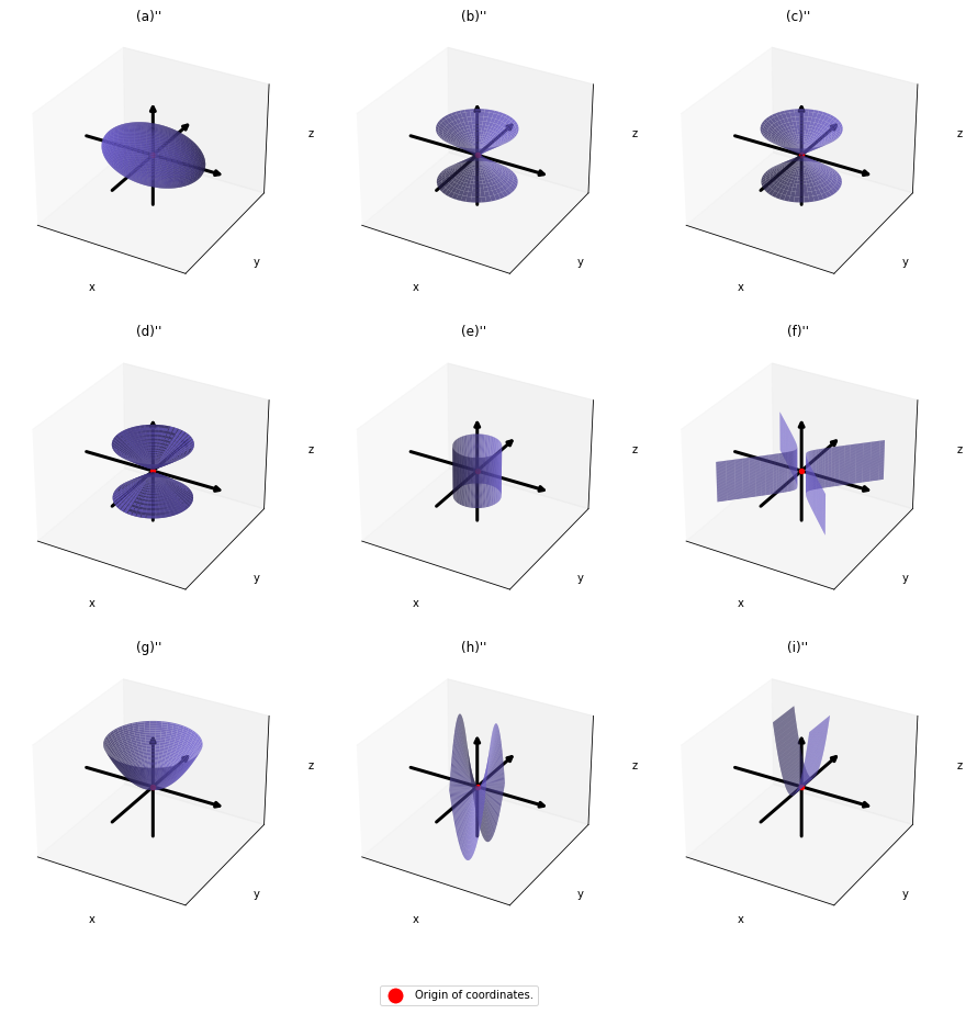
As you could imagine, this is just one simple case of richer variety of graphs. Let’s consider a 3-dimensional space. Any quadratic curves in this space can be denoted as $ax^2 + by^2 + cz^2 + dxy + eyz + fxz + px + qy + rz + s = 0$ , where at least one of $a, b, c, d, e, f, p, q, r, s$ is not $0$ . Let $\boldsymbol{x}$ be $(x, y, z)^T$ , then the quadratic curves can be simply denoted with a $3\times 3$ matrix $A$ and a 3-dimensional vector $\boldsymbol{b}$ as follows: $\boldsymbol{x}^T A\boldsymbol{x} + 2\boldsymbol{b}^T\boldsymbol{x} + s = 0$ , where $A = \left( \begin{array}{ccc} a & \frac{d}{2} & \frac{f}{2} \\ \frac{d}{2} & b & \frac{e}{2} \\ \frac{f}{2} & \frac{e}{2} & c \end{array} \right)$ , $\boldsymbol{b} = \left( \begin{array}{c} \frac{p}{2} \\ \frac{q}{2} \\ \frac{r}{2} \end{array} \right)$ . General quadratic curves are roughly classified into the 9 types below.

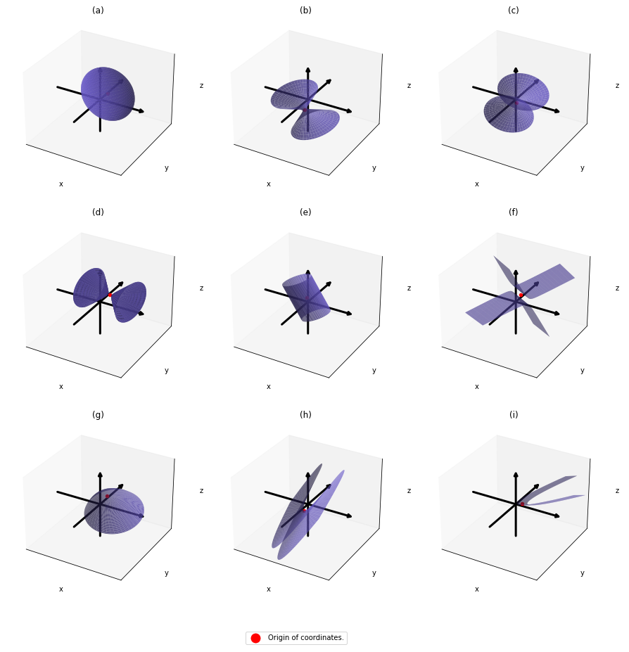
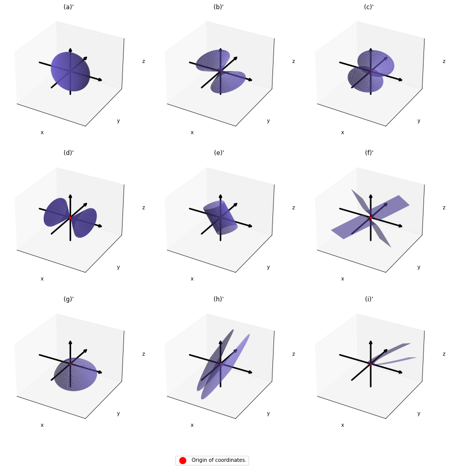
You can shift these quadratic curves so that their center points come to the origin, without rotation, and the resulting curves are as follows. The curves can be all denoted as $\boldsymbol{x}^T A\boldsymbol{x}$ .

As you can see, $A$ is a real symmetric matrix. As I have mentioned repeatedly, when all the elements of a $D \times D$ symmetric matrix $A$ are real values and its eigen values are $\lambda_{i} (i=1, \dots , D)$ , there exist orthogonal/orthonormal matrices $U$ such that $U^{-1}AU = \Lambda$ , where $\Lambda = diag(\lambda_{1}, \dots , \lambda_{D})$ . Hence, you can diagonalize the $A = \left( \begin{array}{ccc} a & \frac{d}{2} & \frac{f}{2} \\ \frac{d}{2} & b & \frac{e}{2} \\ \frac{f}{2} & \frac{e}{2} & c \end{array} \right)$ with an orthogonal matrix $U$ . Let $U$ be an orthogonal matrix such that $U^T A U = \left( \begin{array}{ccc} \alpha & 0 & 0 \\ 0 & \beta & 0 \\ 0 & 0 & \gamma \end{array} \right)$ $=\left( \begin{array}{ccc} \lambda_1 & 0 & 0 \\ 0 & \lambda_2 & 0 \\ 0 & 0 & \lambda_3 \end{array} \right)$ . After you apply rotation by $U$ to the curves (a)” ~ (i)”, those curves are symmetrically placed about the xyz axes, and their center points still cross the origin. The resulting curves look like below. Or rather I should say you projected (a)’ ~ (i)’ on their eigenvectors.

In this article mainly (a)” , (g)”, (h)”, and (i)” are important. General equations for the curves is as follows

(a)”: $\frac{x^2}{l^2} + \frac{y^2}{m^2} + \frac{z^2}{n^2} = 1$
(g)”: $z = \frac{x^2}{l^2} + \frac{y^2}{m^2}$
(h)”: $z = \frac{x^2}{l^2} - \frac{y^2}{m^2}$
(i)”: $z = \frac{x^2}{l^2}$

, where $l, m, n \in \mathbb{R}^+$ .

Even if this section has been puzzling to you, you just have to keep one point in your mind: we have been discussing general quadratic curves, but in PCA, you only need to consider a case where $A$ is a covariance matrix, that is $A=\Sigma$ . PCA corresponds to the case where you shift and rotate the curve (a) into (a)”. Subtracting the mean of data from each point of data corresponds to shifting quadratic curve (a) to (a)’. Calculating eigenvectors of $A$ corresponds to calculating a rotation matrix $U$ such that the curve (a)’ comes to (a)” after applying the rotation, or projecting curves on eigenvectors of $\Sigma$ . Importantly we are only discussing the covariance of certain data, not the distribution of the data itself.

*Just in case you are interested in a little more mathematical sides: it is known that if you rotate all the points $\boldsymbol{x}$ on the curve $\boldsymbol{x}^T A\boldsymbol{x} + 2\boldsymbol{b}^T\boldsymbol{x} + s = 0$ with the rotation matrix $P$ , those points $\boldsymbol{x}$ are mapped into a new quadratic curve $\alpha x^2 + \beta y^2 + \gamma z^2 + \lambda x + \mu y + \nu z + \rho = 0$ . That means the rotation of the original quadratic curve with $P$ (or rather rotating axes) enables getting rid of the terms $xy, yz, zx$ . Also it is known that when $\alpha ' \neq 0$ , with proper translations and rotations, the quadratic curve $\alpha x^2 + \beta y^2 + \gamma z^2 + \lambda x + \mu y + \nu z + \rho = 0$ can be mapped into one of the types of quadratic curves in the figure below, depending on coefficients of the original quadratic curve. And the discussion so far can be generalized to higher dimensional spaces, but that is beyond the scope of this article series. Please consult decent textbooks on linear algebra around you for further details.

4 Eigenvectors are gradients and sometimes variances.

In the second section I explained that you can express quadratic functions $f(\boldsymbol{x}; A) = \boldsymbol{x}^T A \boldsymbol{x}$ in a very simple way by projecting $\boldsymbol{x}$ on eigenvectors of $A$ .

You can comprehend what I have explained in another way: eigenvectors, to be exact eigenvectors of real symmetric matrices $A$ , are gradients. And in case of PCA, I mean when $A=\Sigma$ eigenvalues are also variances. Before explaining what that means, let me explain a little of the totally common facts on mathematics. If you have variables $\boldsymbol{x}\in \mathbb{R}^D$ , I think you can comprehend functions $f(\boldysmbol{x})$ in two ways. One is a normal “functions” $f(\boldsymbol{x})$ , and the others are “curves” $f(\boldsymbol{x}) = const.$ . “Functions” get an input $\boldsymbol{x}$ and gives out an output $f(\boldsymbol{x})$ , just as well as normal functions you would imagine. “Curves” are rather sets of $\boldsymbol{x} \in \mathbb{R}^D$ such that $f(\boldsymbol{x}) = const.$ .

*Please assume that the terms “functions” and “curves” are my original words. I use them just in case I fail to use functions and curves properly.

The quadratic curves in the figure above are all “curves” in my term, which can be denoted as $f(\boldsymbol{x}; A_3, \boldsymbol{b}_3)=const$ or $f(\boldsymbol{x}; A_3)=const$ . However if you replace $z$ of (g)”, (h)”, and (i)” with $f$ , you can interpret the “curves” as “functions” which are denoted as $f(\boldsymbol{x}; A_2)$ . This might sounds too obvious to you, and my point is you can visualize how values of “functions” change only when the inputs are 2 dimensional.

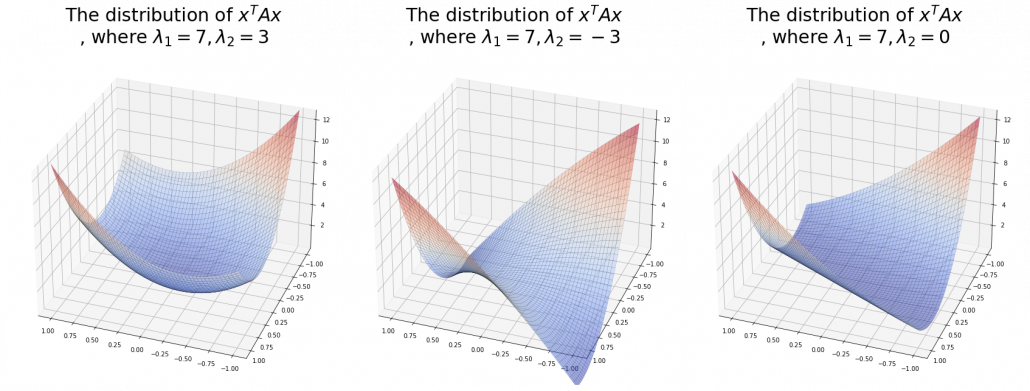
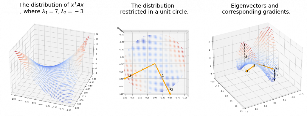
When a symmetric $2\times 2$ real matrices $A_2$ have two eigenvalues $\lambda_1, \lambda_2$ , the distribution of quadratic curves can be roughly classified to the following three types.

(g): Both $\lambda_1$ and $\lambda_2$ are positive or negative.
(h): Either of $\lambda_1$ or $\lambda_2$ is positive and the other is negative.
(i): Either of $\lambda_1$ or $\lambda_2$ is 0 and the other is not.

The equations of (g)” , (h)”, and (i)” correspond to each type of $f=(\boldsymbol{x}; A_2)$ , and thier curves look like the three graphs below.

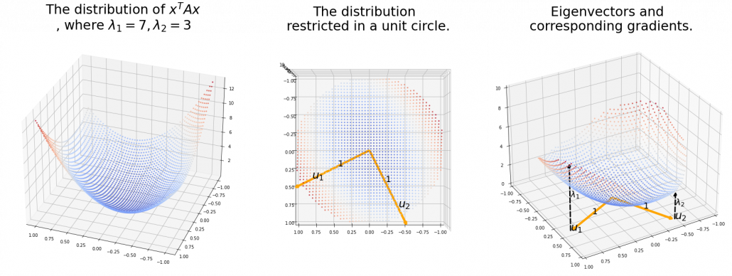
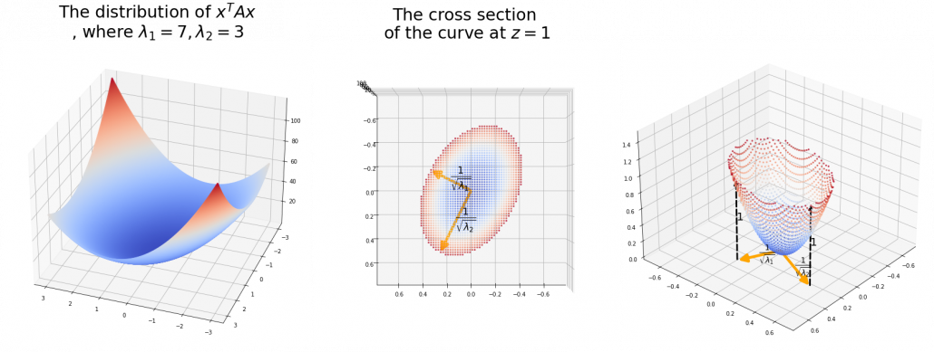
And in fact, when start from the origin and go in the direction of an eigenvector $\boldsymbol{u}_i$ , $\lambda_i$ is the gradient of the direction. You can see that more clearly when you restrict the distribution of $f=(\boldsymbol{x}; A_2)$ to a unit circle. Like in the figure below, in case $\lambda_1 = 7, \lambda_2 = 3$ , which is classified to (g), the distribution looks like the left side, and if you restrict the distribution in the unit circle, the distribution looks like a bowl like the middle and the right side. When you move in the direction of $\boldsymbol{u}_1$ , you can climb the bowl as as high as $\lambda_1$ , in $\boldsymbol{u}_2$ as high as $\lambda_2$ .

Also in case of (h), the same facts hold. But in this case, you can also descend the curve.

*You might have seen the curve above in the context of optimization with stochastic gradient descent. The origin of the curve above is a notorious saddle point, where gradients are all $0$ in any directions but not a local maximum or minimum. Points can be stuck in this point during optimization.

Especially in case of PCA, $A$ is a covariance matrix, thus $A=\Sigma$ . Eigenvalues of $\Sigma$ are all equal to or greater than $0$ . And it is known that in this case $\lambda_i$ is the variance of data projected on its corresponding eigenvector $\boldsymbol{u}_i$ $(i=0, \dots , D)$ . Hence, if you project $f(\boldsymbol{x}; \Sigma)$ , quadratic curves formed by a covariance matrix $\Sigma$ , on eigenvectors of $\Sigma$ , you get $f(\boldsymbol{x}; \Sigma)$ $= ({x'}_1 \: \dots \: {x'}_D) (\lambda_1 {x'}_1 \: \dots \: \lambda_D {x'}_D)^t$ $=\lambda_1 ({x'}_1)^2 + \cdots + \lambda_D ({x'}_D)^2$ . This shows that you can re-weight $({x'}_1 \: \dots \: {x'}_D)$ , the coordinates of data projected projected on eigenvectors of $A$ , with $\lambda_1, \dots, \lambda_D$ , which are variances $({x'}_1 \: \dots \: {x'}_D)$ . As I mentioned in an example of data of exam scores in the last article, the bigger a variance $\lambda_i$ is, the more the feature described by $\boldsymbol{u}_i$ vary from sample to sample. In other words, you can ignore eigenvectors corresponding to small eigenvalues.

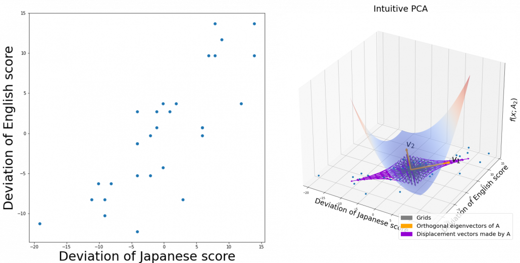
That is a great hint why principal components corresponding to large eigenvectors contain much information of the data distribution. And you can also interpret PCA as a “climbing” a bowl of $f(\boldsymbol{x}; A_D)$ , as I have visualized in the case of (g) type curve in the figure above.

*But as I have repeatedly mentioned, ellipsoid which fit data well is $f(\boldsymbol{x}; \Sigma ^{-1})$ $=(\boldsymbol{x}')^T diag(\frac{1}{\lambda_1}, \dots, \frac{1}{\lambda_D})\boldsymbol{x}'$ $= \frac{({x'}_{1})^2}{\lambda_1} + \cdots + \frac{({x'}_{D})^2}{\lambda_D} = const.$ .

*You have to be careful that even if you slice a type (h) curve $f(\boldsymbol{x}; A_D)$ with a place $z=const.$ the resulting cross section does not fit the original data well because the equation of the cross section is $\lambda_1 ({x'}_1)^2 + \cdots + \lambda_D ({x'}_D)^2 = const.$ The figure below is an example of slicing the same $f(\boldsymbol{x}; A_2)$ as the one above with $z=1$ , and the resulting cross section.

As we have seen, $\lambda_i$ , the eigenvalues of the covariance matrix of data are variances or data when projected on it eigenvectors. At the same time, when you fit an ellipsoid on the data, $\sqrt{\lambda_i}$ is the radius of the ellipsoid corresponding to $\boldsymbol{u}_i$ . Thus ignoring data projected on eigenvectors corresponding to small eigenvalues is equivalent to cutting of the axes of the ellipsoid with small radiusses.

I have explained PCA in three different ways over three articles.

The second article: I focused on what kind of linear transformations convariance matrices $\Sigma$ enable, by visualizing displacement vectors. And those vectors look like swirling and extending into directions of eigenvectors of $\Sigma$ .
The third article: We directly found directions where certain data distribution “swell” the most, to find that data swell the most in directions of eigenvectors.
In this article, we have seen PCA corresponds to only one case of quadratic functions, where the matrix $A$ is a covariance matrix. When you go in the directions of eigenvectors corresponding to big eigenvalues, the quadratic function increases the most. Also that means data samples have bigger variances when projected on the eigenvectors. Thus you can cut off eigenvectors corresponding to small eigenvectors because they retain little information about data, and that is equivalent to fitting an ellipsoid on data and cutting off axes with small radiuses.

*Let $A$ be a covariance matrix, and you can diagonalize it with an orthogonal matrix $U$ as follow: $U^{T}AU = \Lambda$ , where $\Lambda = diag(\lambda_1, \dots, \lambda_D)$ . Thus $A = U \Lambda U^{T}$ . $U$ is a rotation, and multiplying a $\boldsymbol{x}$ with $\Lambda$ means you multiply each eigenvalue to each element of $\boldsymbol{x}$ . At the end $U^T$ enables the reverse rotation.

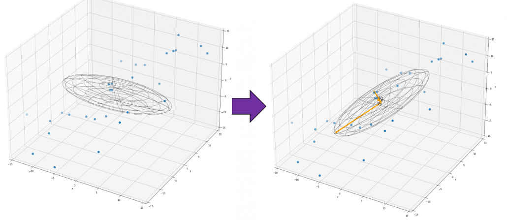
If you get data like the left side of the figure below, most explanation on PCA would just fit an oval on this data distribution. However after reading this articles series so far, you would have learned to see PCA from different viewpoints like at the right side of the figure below.

5 Ellipsoids in Gaussian distributions.

I have explained that if the covariance of a data distribution is $\boldsymbol{\Sigma}$ , the ellipsoid which fits the distribution the best is $\bigl((\boldsymbol{x} - \boldsymbol{\mu}), \boldsymbol{\Sigma}^{-1}(\boldsymbol{x} - \boldsymbol{\mu})\bigr) = 1$ . You might have seen the part $\bigl((\boldsymbol{x} - \boldsymbol{\mu}), \boldsymbol{\Sigma}^{-1}(\boldsymbol{x} - \boldsymbol{\mu})\bigr) =$ $(\boldsymbol{x} - \boldsymbol{\mu}) \boldsymbol{\Sigma}^{-1}(\boldsymbol{x} - \boldsymbol{\mu})$ somewhere else. It is the exponent of general Gaussian distributions: $\mathcal{N}(\boldsymbol{x} | \boldsymbol{\mu}, \boldsymbol{\Sigma}) =$ $\frac{1}{(2\pi)^{D/2}} \frac{1}{|\boldsymbol{\Sigma}|} exp\{ -\frac{1}{2}(\boldsymbol{x} - \boldsymbol{\mu}) \boldsymbol{\Sigma}^{-1}(\boldsymbol{x} - \boldsymbol{\mu}) \}$ . It is known that the eigenvalues of $\Sigma ^{-1}$ are $\frac{1}{\lambda_1}, \dots, \frac{1}{\lambda_D}$ , and eigenvectors corresponding to each eigenvalue are also $\boldsymbol{u}_1, \dots, \boldsymbol{u}_D$ respectively. Hence just as well as what we have seen, if you project $(\boldsymbol{x} - \boldsymbol{\mu})$ on each eigenvector of $\Sigma ^{-1}$ , we can convert the exponent of the Gaussian distribution.

Let $-\frac{1}{2}(\boldsymbol{x} - \boldsymbol{\mu}) \boldsymbol{\Sigma}^{-1}(\boldsymbol{x} - \boldsymbol{\mu})$ be $\boldsymbol{y}$ and $U ^{-1} \boldsymbol{y}= U^{T} \boldsymbol{y}$ be $\boldsymbol{y}'$ , where $U=(\boldsymbol{u}_1 \: \dots \: \boldsymbol{u}_D)$ . Just as we have seen, $(\boldsymbol{x} - \boldsymbol{\mu}) \boldsymbol{\Sigma}^{-1}(\boldsymbol{x} - \boldsymbol{\mu})$ $=\boldsymbol{y}^T\Sigma^{-1} \boldsymbol{y}$ $=(U\boldsymbol{y}')^T \Sigma^{-1} U\boldsymbol{y}'$ $=((\boldsymbol{y}')^T U^T \Sigma^{-1} U\boldsymbol{y}'$ $= (\boldsymbol{y}')^T diag(\frac{1}{\lambda_1}, \dots, \frac{1}{\lambda_D}) \boldsymbol{y}'$ $= \frac{({y'}_{1})^2}{\lambda_1} + \cdots + \frac{({y'}_{D})^2}{\lambda_D}$ . Hence $\mathcal{N}(\boldsymbol{x} | \boldsymbol{\mu}, \boldsymbol{\Sigma}) =$ $\frac{1}{(2\pi)^{D/2}} \frac{1}{|\boldsymbol{\Sigma}|} exp\{ -\frac{1}{2}(\boldsymbol{y}) \boldsymbol{\Sigma}^{-1}(\boldsymbol{y}) \} = \frac{1}{(2\pi)^{D/2}} \frac{1}{|\boldsymbol{\Sigma}|} exp\{ -\frac{1}{2}(\frac{({y'}_{1})^2}{\lambda_1} + \cdots + \frac{({y'}_{D})^2}{\lambda_D} ) \}$ $=\frac{1}{(2\pi)^{1/2}} \frac{1}{|\boldsymbol{\Sigma}|} exp\biggl( -\frac{1}{2} \frac{({y'}_{1})^2}{\lambda_1} \biggl) \cdots \frac{1}{(2\pi)^{1/2}} \frac{1}{|\boldsymbol{\Sigma}|} exp\biggl( -\frac{1}{2}\frac{({y'}_{D})^2}{\lambda_D} \biggl)$ .

*To be mathematically exact about changing variants of normal distributions, you have to consider for example Jacobian matrices.

This results above demonstrate that, by projecting data on the eigenvectors of its covariance matrix, you can factorize the original multi-dimensional Gaussian distribution into a product of Gaussian distributions which are irrelevant to each other. However, at the same time, that is the potential limit of approximating data with PCA. This idea is going to be more important when you think about more probabilistic ways to handle PCA, which is more robust to lack of data.

I have explained PCA over 3 articles from various viewpoints. If you have been patient enough to read my article series, I think you have gained some deeper insight into not only PCA, but also linear algebra, and that should be helpful when you learn or teach data science. I hope my codes also help you. In fact these are not the only topics about PCA. There are a lot of important PCA-like algorithms.

In fact our expedition of ellipsoids, or PCA still continues, just as Star Wars series still continues. Especially if I have to explain an algorithm named probabilistic PCA, I need to explain the “Bayesian world” of machine learning. Most machine learning algorithms covered by major introductory textbooks tend to be too deterministic and dependent on the size of data. Many of those algorithms have another “parallel world,” where you can handle inaccuracy in better ways. I hope I can also write about them, and I might prepare another trilogy for such PCA. But I will not disappoint you, like “The Phantom Menace.”

Appendix: making a model of a bunch of grape with ellipsoid berries.

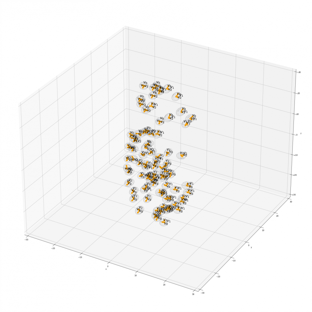
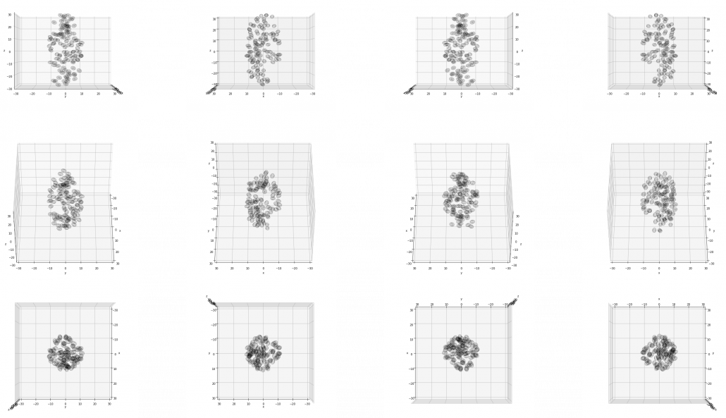
If you can control quadratic curves, reshaping and rotating them, you can make a model of a grape of olive bunch on Matplotlib. I made a program of making a model of a bunch of berries on Matplotlib using the module to draw ellipsoids which I introduced earlier. You can check the codes in this page.

*I have no idea how many people on this earth are in need of making such models.

I made some modules so that you can see the grape bunch from several angles. This might look very simple to you, but the locations of berries are organized carefully so that it looks like they are placed around a stem and that the berries are not too close to each other.

The programming code I created for this article is completly available here.

[Refereces]

[1]C. M. Bishop, “Pattern Recognition and Machine Learning,” (2006), Springer, pp. 78-83, 559-577

[2]「理工系新課程　線形代数　基礎から応用まで」, 培風館、(2017)

[3]「これなら分かる　最適化数学　基礎原理から計算手法まで」, 金谷健一著、共立出版, (2019), pp. 17-49

[4]「これなら分かる　応用数学教室　最小二乗法からウェーブレットまで」, 金谷健一著、共立出版, (2019), pp.165-208

[5] 「サボテンパイソン」
https://sabopy.com/

The algorithm known as PCA and my taxonomy of linear dimension reductions

November 23, 2020/in Artificial Intelligence, Big Data, Data Mining, Data Science, Machine Learning, Main Category, Mathematics, Statistics/by Yasuto Tamura

In one of my previous articles, I explained the importance of reducing dimensions. Principal Component Analysis (PCA) and Linear Discriminant Analysis (LDA) are the simplest types of dimension reduction algorithms. In upcoming articles of mine, you are going to see what these algorithms do. In conclusion, diagonalization, which I mentioned in the last article, is what these algorithms are all about, but still in this article I can mainly cover only PCA.

This article is largely based on the explanations in Pattern Recognition and Machine Learning by C. M. Bishop (which is often called “PRML”), and when you search “PCA” on the Internet, you will find more or less similar explanations. However I hope I can go some steps ahead throughout this article series. I mean, I am planning to also cover more generalized versions of PCA, meanings of diagonalization, the idea of subspace. I believe this article series is also effective for refreshing your insight into linear algebra.

*This is the third article of my article series “Illustrative introductions on dimension reduction.”

1. My taxonomy on linear dimension reduction

*If you soon want to know what the algorithm called “PCA” is, you should skip this section for now to avoid confusion.

Out of the two algorithms I mentioned, PCA is especially important and you would see the same or similar ideas in various fields such as signal processing, psychology, and structural mechanics. However in most cases, the word “PCA” refers to one certain algorithm of linear dimension reduction. Most articles or study materials only mention the “PCA,” and this article is also going to cover only the algorithm which most poeple call “PCA.” However I found that PCA is only one branch of linear dimension reduction algorithms.

*From now on all the terms “PCA” in this article means the algorithm known as PCA unless I clearly mention the generalized KL transform.

*This chart might be confusing to you. According to PRML, PCA and KL transform is identical. PCA has two formulations, maximum variance formulation and minimum error formulation, and they can give the same result. However according to a Japanese textbook, which is very precise about this topic, KL transform has two formulations, and what we call PCA is based on maximum variance formulation. I am still not sure about correct terminology, but in this article I am going to call the most general algorithm “generalized KL transform,” I mean the root of the chart above.

*Most materials just explain the most major PCA, but if you consider this generalized KL transform, I can introduce an intriguing classification algorithm called subspace method. This algorithm was invented in Japan, and this is not so popular in machine learning textbooks in general, but learning this method would give you better insight into the idea of multidimensional space in machine learning. In the future, I am planning to cover this topic in this article series.

2. PCA

When someones mention “PCA,” I am sure for the most part that means the algorithm I am going to explain in the rest of this article. The most intuitive and straightforward way to explain PCA is that, PCA (Principal Component Analysis) of two or three dimensional data is fitting an oval to two dimensional data or fitting an ellipsoid to three dimensional data. You can actually try to plot some random dots on a piece of paper, and draw an oval which fits the dots the best. Assume that you have these 2 or 3 dimensional data below, and please try to put an oval or an ellipsoid to the data.

I think this is nothing difficult, but I have a question: what was the logic behind your choice?

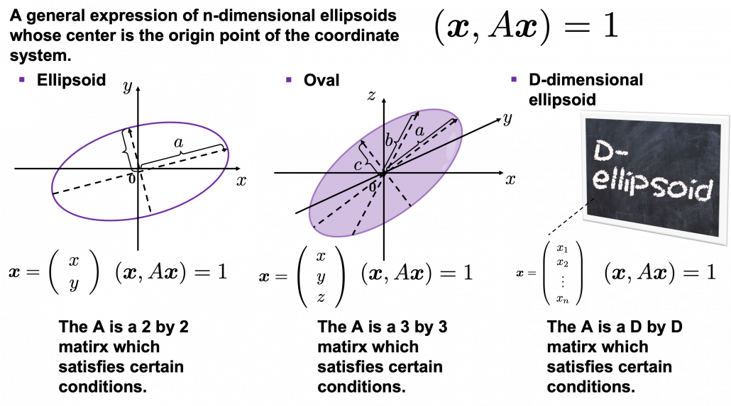
Some might have roughly drawn its outline. Formulas of “the surface” of general ellipsoids can be explained in several ways, but in this article you only have to consider ellipsoids whose center is the origin point of the coordinate system. In PCA you virtually shift data so that the mean of the data comes to the origin point of the coordinate system. When $A$ is a certain type of $D\times D$ matrix, the formula of a D-dimensional ellipsoid whose center is identical to the origin point is as follows: $(\boldsymbol{x}, A\boldsymbol{x}) = 1$ , where $\boldsymbol{x}\in \mathbb{R}$ . As is always the case with formulas in data science, you can visualize such ellipsoids if you are talking about 1, 2, or 3 dimensional data like in the figure below, but in general D-dimensional space, it is theoretical/imaginary stuff on blackboards.

*In order to explain the conditions which the matrix $A$ has to hold, I need another article, so for now please just assume that the $A$ is a kind of magical matrix.

You might have seen equations of 2 or 3 dimensional ellipsoids in the following way: $\frac{x^2}{a^2} + \frac{y^2}{b^2} = 1$ , where $a\neq 0, b\neq 0$ or $\frac{x^2}{a^2} + \frac{y^2}{b^2} + \frac{z^2}{c^2}= 1$ , where $a\neq 0, b\neq 0, c \neq 0$ . These are special cases of the equation $(\boldsymbol{x}, A\boldsymbol{x}) = 1$ , where $A=diag(a_1^2, \dots, a_D^2)$ . In this case the axes of ellipsoids the same as those of the coordinate system. Thus in this simple case, $A=diag(a^2, b^2)$ or $A=diag(a^2,c^2,c^2)$ .

I am going explain these equations in detail in the upcoming articles. But thre is one problem: how would you fit an ellipsoid when a data distribution does not look like an ellipsoid?

In fact we have to focus more on another feature of ellipsoids: all the axes of an ellipsoid are orthogonal. In conclusion the axes of the ellipsoids are more important in PCA, so I do want you to forget about the surface of ellipsoids for the time being. You might get confused if you also think about the surface of ellipsoid now. I am planning to cover this topic in the next article. I hope this article, combined with the last one and the next one, would help you have better insight into the ideas which frequently appear in data science or machine learning context.

3. Fitting orthogonal axes on data

*If you have no trouble reading the chapter 12.1 of PRML, you do not need to this section or maybe even this article, but I hope at least some charts or codes of mine would enhance your understanding on this topic.

*I must admit I wrote only the essence of PCA formulations. If that seems too abstract to you, you should just breifly read through this section and go to the next section with a more concrete example. If you are confused, there should be other good explanations on PCA on the internet, and you should also check them. But at least the visualization of PCA in the next section would be helpful.

As I implied above, all the axes of ellipsoids are orthogonal, and selecting the orthogonal axes which match data is what PCA is all about. And when you choose those orthogonal axes, it is ideal if the data look like an ellipsoid. Simply putting we want the data to “swell” along the axes.

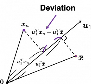
Then let’s see how to let them “swell,” more mathematically. Assume that you have 2 dimensional data plotted on a coordinate system $(\boldsymbol{e}_1, \boldsymbol{e}_2)$ as below (The samples are plotted in purple). Intuitively, the data “swell” the most along the vector $\boldsymbol{u}_1$ . Also it is clear that $\boldsymbol{u}_2$ is the only vector orthogonal to $\boldsymbol{u}_1$ . We can expect that the new coordinate system $(\boldsymbol{u}_1, \boldsymbol{u}_2)$ expresses the data in a better way, and you you can get new coordinate points of the samples by projecting them on new axes as done with yellow lines below.

Next, let’s think about a case in 3 dimensional data. When you have 3 dimensional data in a coordinate system $(\boldsymbol{e}_1, \boldsymbol{e}_2,\boldsymbol{e}_3)$ as below, the data “swell” the most also along $\boldsymbol{u}_1$ . And the data swells the second most along $\boldsymbol{u}_2$ . The two axes, or vectors span the plain in purple. If you project all the samples on the plain, you will get 2 dimensional data at the right side. It is important that we did not consider the third axis. That implies you might be able to display the data well with only 2 dimensional sapce, which is spanned by the two axes $\boldsymbol{v}_1, \boldsymbol{v}_2$ .

Thus the problem is how to calculate such axis $\boldsymbol{u}_1$ . We want the variance of data projected on $\boldsymbol{u}_1$ to be the biggest. The coordinate of $\boldsymbol{x}_n$ on the axis $\boldsymbol{u}_1$ . The coordinate of a data point $\boldsymbol{x}_n$ on the axis $\boldsymbol{u}_1$ is calculated by projecting $\boldsymbol{x}_n$ on $\boldsymbol{u}_1$ . In data science context, such projection is synonym to taking an inner product of $\boldsymbol{x}_n$ and $\boldsymbol{u}_1$ , that is calculating $\boldsymbol{u}_1^T \boldsymbol{x}_n$ .

*Each element of $\boldsymbol{x}_n$ is the coordinate of the data point $\boldsymbol{x}_n$ in the original coordinate system. And the projected data on $\boldsymbol{u}_1$ whose coordinates are 1-dimensional correspond to only one element of transformed data.

To calculate the variance of projected data on $\boldsymbol{u}_1$ , we just have to calculate the mean of variances of 1-dimensional data projected on $\boldsymbol{u}_1$ . Assume that $\bar{\boldsymbol{x}}$ is the mean of data in the original coordinate, then the deviation of $\boldsymbol{x}_1$ on the axis $\boldsymbol{u}_1$ is calculated as $\boldsymbol{u}_1^T \boldsymbol{x}_n - \boldsymbol{u}_1^T \bar{\boldsymbol{x}}$ , as shown in the figure. Hence the variance, I mean the mean of the deviation on is $\frac{1}{N} \sum^{N}_{n}{\boldsymbol{u}_1^T \boldsymbol{x}_n - \boldsymbol{u}_1^T \bar{\boldsymbol{x}}}$ , where $N$ is the total number of data points. After some deformations, you get the next equation $\frac{1}{N} \sum^{N}_{n}{\boldsymbol{u}_1^T \boldsymbol{x}_n - \boldsymbol{u}_1^T \bar{\boldsymbol{x}}} = \boldsymbol{u}_1^T S \boldsymbol{u}_1$ , where $S = \frac{1}{N}\sum_{n=1}^{N}{(\boldsymbol{x}_n - \bar{\boldsymbol{x}})(\boldsymbol{x}_n - \bar{\boldsymbol{x}})^T}$ . $S$ is known as a covariance matrix.

We are now interested in maximizing the variance of projected data on $\boldsymbol{u}_1^T S \boldsymbol{u}_1$ , and for mathematical derivation we need some college level calculus, so if that is too much for you, you can skip reading this part till the next section.

We now want to calculate $\boldsymbol{u}_1$ with which $\boldsymbol{u}_1^T S \boldsymbol{u}_1$ is its maximum value. General $\boldsymbol{u}_i$ including $\boldsymbol{u}_1$ are just coordinate axes after PCA, so we are just interested in their directions. Thus we can set one constraint $\boldsymbol{u}_1^T \boldsymbol{u}_1 = 1$ . Introducing a Lagrange multiplier, we have only to optimize next problem: $\boldsymbol{u}_1 ^ {*} = \mathop{\rm arg~max}\limits_{\boldsymbol{u}_1} \{ \boldsymbol{u}_1^T S \boldsymbol{u}_1 + \lambda_1 (1 - \boldsymbol{u}_1^T \boldsymbol{u}_1) \}$ . In conclusion $\boldsymbol{u}_1 ^ {*}$ satisfies $S\boldsymbol{u}_1 ^ {*} = \lamba_1 \boldsymbol{u}_1 ^ {*}$ . If you have read my last article on eigenvectors, you wold soon realize that this is an equation for calculating eigenvectors, and that means $\boldsymbol{u}_1 ^ {*}$ is one of eigenvectors of the covariance matrix S. Given the equation of eigenvector the next equation holds $\boldsymbol{u}_1 ^ {*}^T S \boldsymbol{u}_1 ^ {*} = \lambda_1$ . We have seen that $\boldsymbol{u}_1 ^T S \boldsymbol{u}_1 ^$ is a the variance of data when projected on a vector $\boldsymbol{u}_1$ , thus the eigenvalue $\lambda_1$ is the biggest variance possible when the data are projected on a vector.

Just in the same way you can calculate the next biggest eigenvalue $\lambda_2$ , and it it the second biggest variance possible, and in this case the date are projected on $\boldsymbol{u}_2$ , which is orthogonal to $\boldsymbol{u}_1$ . As well you can calculate orthogonal 3rd 4th …. Dth eigenvectors.

*To be exact I have to explain the cases where we can get such D orthogonal eigenvectors, but that is going to be long. I hope I can to that in the next article.

4. Practical three dimensional example of PCA

We have seen that PCA is sequentially choosing orthogonal axes along which data points swell the most. Also we have seen that it is equal to calculating eigenvalues of the covariance matrix of the data from the largest to smallest one. From now on let’s work on a practical example of data. Assume that we have 30 students’ scores of Japanese, math, and English tests as below.

* I think the subject “Japanese” is equivalent to “English” or “language art” in English speaking countries, and maybe “Deutsch” in Germany. This example and the explanation are largely based on a Japanese textbook named 「これなら分かる応用数学教室　最小二乗法からウェーブレットまで」. This is a famous textbook with cool and precise explanations on mathematics for engineering. Partly sharing this is one of purposes of this article.

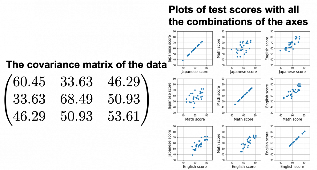
At the right side of the figure below is plots of the scores with all the combinations of coordinate axes. In total 9 inverse graphs are symmetrically arranged in the figure, and it is easy to see that English & Japanese or English and math have relatively high correlation. The more two axes have linear correlations, the bigger the covariance between them is.

In the last article, I visualized the eigenvectors of a $3\times 3$ matrix $A = \frac{1}{50} \begin{pmatrix} 60.45 & 33.63 & 46.29 \\33.63 & 68.49 & 50.93 \\ 46.29 & 50.93 & 53.61 \end{pmatrix}$ , and in fact the matrix is just a constant multiplication of this covariance matrix. I think now you understand that PCA is calculating the orthogonal eigenvectors of covariance matrix of data, that is diagonalizing covariance matrix with orthonormal eigenvectors. Hence we can guess that covariance matrix enables a type of linear transformation of rotation and expansion and contraction of vectors. And data points swell along eigenvectors of such matrix.

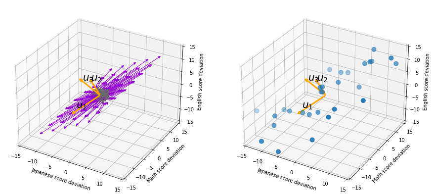
Then why PCA is useful? In order to see that at first, for simplicity assume that $x, y, z$ denote Japanese, Math, English scores respectively. The mean of the data is $\left( \begin{array}{c} \bar{x} \\ \bar{y} \\ \bar{z} \end{array} \right) = \left( \begin{array}{c} 58.1 \\ 61.8 \\ 67.3 \end{array} \right)$ , and the covariance matrix of data in the original coordinate system is $V_{xyz} = \begin{pmatrix} 60.45 & 33.63 & 46.29 \\33.63 & 68.49 & 50.93 \\ 46.29 & 50.93 & 53.61 \end{pmatrix}$ . The eigenvalues of $V_{xyz}$ are $\lambda_1=148.34, \lambda_2 = 30.62$ , and $\lambda_3 = 3.60$ , and their corresponding unit eigenvectors are $\boldsymbol{u}_1 = \left( \begin{array}{c} 0.540 \\ 0.602 \\ 0.589 \end{array} \right) , \boldsymbol{u}_2 = \left( \begin{array}{c} 0.736 \\ -0.677 \\ 0.0174 \end{array} \right) , \boldsymbol{u}_3 = \left( \begin{array}{c} -0.408 \\ -0.4.23 \\ 0.809 \end{array} \right)$ respectively. $U = (\boldsymbol{u}_1 \quad \boldsymbol{u}_2 \quad \boldsymbol{u}_3 )$ is an orthonormal matrix, where $\boldsymbol{u}_i^T\boldsymbol{u}_j = \begin{cases} 1 & (i=j) \\ 0 & (otherwise) \end{cases}$ . As I explained in the last article, you can diagonalize $V_{xyz}$ with $U$ : $U^T V_{xyz}U = diag(\lambda_1, \dots, \lambda_D)$ .

In order to see how PCA is useful, assume that $\left( \begin{array}{c} \xi \\ \eta \\ \zeta \end{array} \right) = U^T \left( \begin{array}{c} x - \bar{x} \\ y - \bar{y} \\ z - \bar{z} \end{array} \right)$ .

Let’s take a brief look at what a linear transformation by $U^T$ means. Each element of $\boldsymbol{x}$ denotes coordinate of the data point $\boldsymbol{x}$ in the original coordinate system (In this case the original coordinate system is composed of $\boldsymbol{e}_1, \boldsymbol{e}_2$ , and $\boldsymbol{e}_3$ ). $U = (\boldsymbol{u}_1, \boldsymbol{u}_2, \boldsymbol{u}_3)$ enables a rotation of a rigid body, which means the shape or arrangement of data will not change after the rotation, and $U^T$ enables a reverse rotation of the rigid body.

*Roughly putting, if you hold a bold object such as a metal ball and rotate your arm, that is a rotation of a rigid body, and your shoulder is the origin point. On the other hand, if you hold something soft like a marshmallow, it would be squashed in your hand, and that is not a not a rotation of a rigid body.

You can rotate $\boldsymbol{x}$ with $U$ like $U^T\boldsymbol{x} = \left( \begin{array}{c} -\boldsymbol{u}_1^{T}- \\ -\boldsymbol{u}_2^{T}- \\ -\boldsymbol{u}_3^{T}- \end{array} \right)\boldsymbol{x}=\left( \begin{array}{c} \boldsymbol{u}_1^{T}\boldsymbol{x} \\ \boldsymbol{u}_2^{T}\boldsymbol{x} \\ \boldsymbol{u}_3^{T}\boldsymbol{x} \end{array} \right)$ , and $\boldsymbol{u}_i^{T}\boldsymbol{x}$ is the coordinate of $\boldsymbol{x}$ projected on the axis $\boldsymbol{u}_i$ .

Let’s see this more visually. Assume that the data point $\boldsymbol{x}$ is a purple dot and its position is expressed in the original coordinate system spanned by black arrows . By multiplying $\boldsymbol{x}$ with $U^T$ , the purple point $\boldsymbol{x}$ is projected on the red axes respectively, and the product $\left( \begin{array}{c} \boldsymbol{u}_1^{T}\boldsymbol{x} \\ \boldsymbol{u}_2^{T}\boldsymbol{x} \\ \boldsymbol{u}_3^{T}\boldsymbol{x} \end{array} \right)$ denotes the coordinate point of the purple point in the red coordinate system. $\boldsymbol{x}$ is rotated this way, but for now I think it is better to think that the data are projected on new coordinate axes rather than the data themselves are rotating.

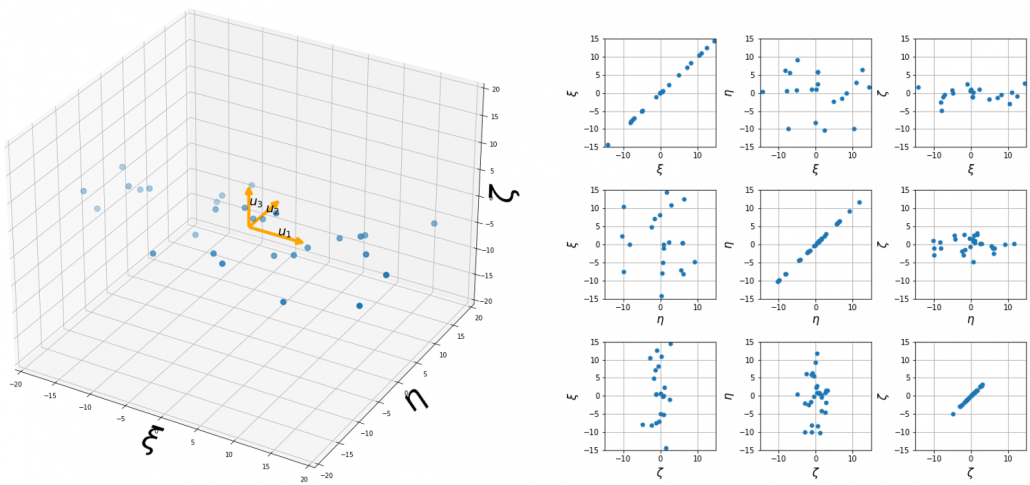
Now that we have seen what rotation by $U$ means, you should have clearer image on what $\left( \begin{array}{c} \xi \\ \eta \\ \zeta \end{array} \right) = U^T \left( \begin{array}{c} x - \bar{x} \\ y - \bar{y} \\ z - \bar{z} \end{array} \right)$ means. $\left( \begin{array}{c} \xi \\ \eta \\ \zeta \end{array} \right)$ denotes the coordinates of data projected on new axes $\boldsymbol{u}_1, \boldsymbol{u}_2, \boldsymbol{u}_3$ , which are unit eigenvectors of $V_{xyz}$ . In the coordinate system spanned by the eigenvectors, the data distribute like below.

By multiplying $U$ from both sides of the equation above, we get $\left( \begin{array}{c} x - \bar{x} \\ y - \bar{y} \\ z - \bar{z} \end{array} \right) =U \left( \begin{array}{c} \xi \\ \eta \\ \zeta \end{array} \right)$ , which means you can express deviations of the original data as linear combinations of the three factors $\xi, \eta$ , and $\zeta$ . We expect that those three factors contain keys for understanding the original data more efficiently. If you concretely write down all the equations for the factors: $\xi = 0.540 (x - \bar{x}) + 0.602 (y - \bar{y}) + 0.588 (z - \bar{z})$ , $\eta = 0.736(x - \bar{x}) - 0.677 (y - \bar{y}) + 0.0174 (z - \bar{z})$ , and $\zeta = - 0.408 (x - \bar{x}) - 0.423 (y - \bar{y}) + 0.809(z - \bar{z})$ . If you examine the coefficients of the deviations $(x - \bar{x}), (y - \bar{y})$ , and $(z - \bar{z})$ , we can observe that $\eta$ almost equally reflects the deviation of the scores of all the subjects, thus we can say $\eta$ is a factor indicating one’s general academic level. When it comes to $\eta$ Japanese and Math scores are important, so we can guess that this factor indicates whether the student is at more of “scientific side” or “liberal art side.” In the same way $\zeta$ relatively makes much of one’s English score, so it should show one’s “internationality.” However the covariance of the data $\xi, \eta, \zeta$ is $V_{\xi \eta \zeta} = \begin{pmatrix} 148.34 & 0 & 0 \\ 0 & 30.62 & 0 \\ 0 & 0 & 3.60 \end{pmatrix}$ . You can see $\zeta$ does not vary from students to students, which means it is relatively not important to describe the tendency of data. Therefore for dimension reduction you can cut off the factor $\zeta$ .

*Assume that you can apply PCA on D-dimensional data and that you get $\boldsymbol{x}'$ , where $\boldsymbol{x}' = U^T\boldsymbol{x} - \bar{\boldsymbol{x}}$ . The variance of data projected on new D-dimensional coordinate system is $V'=\frac{1}{N}\sum{(\boldsymbol{x}')^T\boldsymbol{x}'}$ $=\frac{1}{N}\sum{(U^T\boldsymbol{x})^T(U^T\boldsymbol{x})}$ $=\frac{1}{N}\sum{U^T\boldsymbol{x}\boldsymbol{x}^TU}$ $=U^T(\frac{1}{N}\sum{\boldsymbol{x}\boldsymbol{x}^T})U$ $=U^TVU$ $=diag(\lambda_1, \dots, \lambda_D)$ . This means that in the new coordinate system after PCA, covariances between any pair of variants are all zero.

*As I mentioned $U$ is a rotation of a rigid body, and $U^T$ is the reverse rotation, hence $U^TU = UU^T = I$ .

Hence you can approximate the original 3 dimensional data on the coordinate system $(\boldsymbol{e}_1, \boldsymbol{e}_2, \boldsymbol{e}_3)$ from the reduced two dimensional coordinate system $(\boldsymbol{u}_1, \boldsymbol{u}_2)$ with the following equation: $\left( \begin{array}{c} x - \bar{x} \\ y - \bar{y} \\ z - \bar{z} \end{array} \right) \approx U_{reduced} \left( \begin{array}{c} \xi \\ \eta \end{array} \right) = (\boldsymbol{u}_1 \quad \boldsymbol{u}_2) \left( \begin{array}{c} \xi \\ \eta \end{array} \right)$ . Then it mathematically clearer that we can express the data with two factors: “how smart the student is” and “whether he is at scientific side or liberal art side.”

We can observe that eigenvalue $\lambda_i$ is a statistic which indicates how much the corresponding $\boldsymbol{u}_i$ can express the data, $\frac{\lambda_i}{\sum_{j=1}^{D}{\lambda_j}}$ is called the contribution ratio of eigenvector $\boldsymbol{u}_i$ . In the example above, the contribution ratios of $\boldsymbol{u}_1, \boldsymbol{u}_2,$ and $\boldsymbol{u}_3$ are respectively $\frac{\lambda_1}{\lambda_1 + \lambda_2 + \lambda_3}=0.813$ , $\frac{\lambda_2}{\lambda_1 + \lambda_2 + \lambda_3}=0.168$ , $\frac{\lambda_3}{\lambda_1 + \lambda_2 + \lambda_3}=0.0197$ . You can decide how many degrees of dimensions you reduce based on this information.

Appendix: Playing with my toy PCA on MNIST dataset

Applying “so called” PCA on MNIST dataset is a super typical topic that many other tutorial on PCA also introduce, but I still recommend you to actually implement, or at least trace PCA implementation with MNIST dataset without using libraries like scikit-learn. While reading this article I recommend you to actually run the first and the second code below. I think you can just copy and paste them on your tool to run Python, installing necessary libraries. I wrote them on Jupyter Notebook.

In my implementation, in the simple configuration part you can set the USE_ALL_NUMBERS as True or False boolean. If you set it as True, you apply PCA on all the data of numbers from 0 to 9. If you set it as True, you can specify which digit to apply PCA on. In this article, I show the results results of PCA on the data of digit ‘3.’ The first three images of ‘3’ are as below.

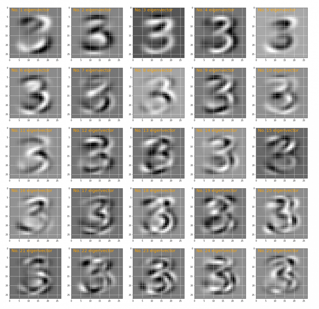
You have to keep it in mind that the data are all shown as 28 by 28 pixel grayscale images, but in the process of PCA, they are all processed as 28 * 28 = 784 dimensional vectors. After applying PCA on the 784 dimensional vectors of images of ‘3,’ the first 25 eigenvectors are as below. You can see that at the beginning the eigenvectors partly retain the shapes of ‘3,’ but they are distorted as the eigenvalues get smaller. We can guess that the latter eigenvalues are not that helpful in reconstructing the shape of ‘3.’

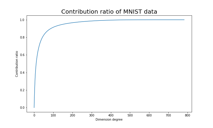
Just as we saw in the last section, you you can cut off axes of eigenvectors with small eigenvalues and reduce the dimension of MNIST data. The figure below shows how contribution ratio of MNIST data grows. You can see that around 200 dimension degree, the contribution ratio reaches around 0.95. Then we can guess that even if we reduce the dimension of MNIST from 784 to 200 we can retain the most of the structure of original data.

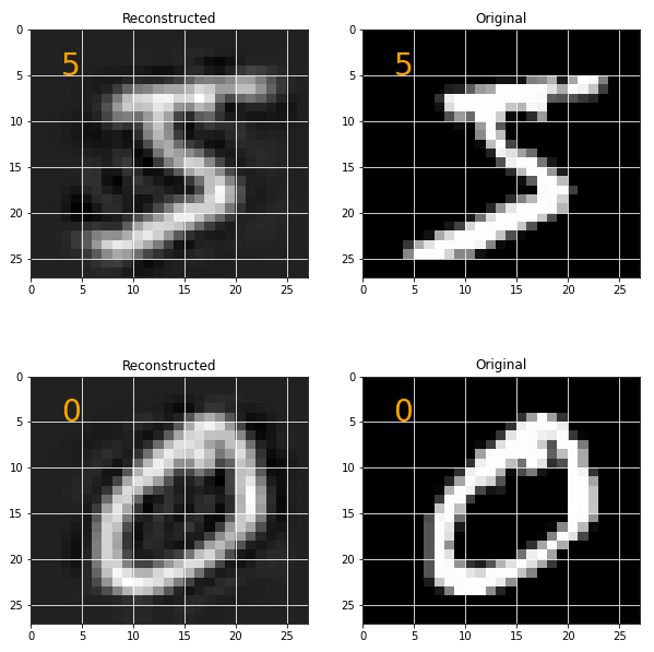
Some results of reconstruction of data from 200 dimensional space are as below. You can set how many images to display by adjusting NUMBER_OF_RESULTS in the code. And if you set LATENT_DIMENSION as 784, you can completely reconstruct the data.

* I make study materials on machine learning, sponsored by DATANOMIQ. I do my best to make my content as straightforward but as precise as possible. I include all of my reference sources. If you notice any mistakes in my materials, including grammatical errors, please let me know (email: yasuto.tamura@datanomiq.de). And if you have any advice for making my materials more understandable to learners, I would appreciate hearing it.

*I attatched the codes I used to make the figures in this article. You can just copy, paste, and run, sometimes installing necessary libraries.

import numpy as np

import keras # There should be some other simpler ways to download MNIST dataset,

# but at least on my laptop, this was the easiest.

import matplotlib.pyplot as plt

# Configuration part

USE_ALL_NUMBERS = False

WHICH_NUMBER = 3

W_RAW_DATA = 3

H_RAW_DATA = 1 # 1<= W_RAW_DATA*H_RAW_DATA <= 28*28

H_EIGENVECTORS = 5

W_EIGENVECTORS = 5 # 1<= H_EIGENVECTORS*W_EIGENVECTORS <= 28*28

# Preparing data

mnist = keras.datasets.mnist

(data, labels), (_, _) = mnist.load_data()

data = data.reshape([-1, 28*28])

if USE_ALL_NUMBERS:

data_to_use = data

labels_to_use = labels

else:

data_to_use = data[labels==WHICH_NUMBER]

labels_to_use = labels[labels==WHICH_NUMBER]

# Applying PCA to the data to use

ave = np.mean(data_to_use, axis=0)

covariance_matrix = np.dot((data_to_use - ave).T, (data_to_use - ave))

eigen_values, eigen_vectors = np.linalg.eig(covariance_matrix)

sorted_index = eigen_values.argsort()[::-1]

eigen_values=eigen_values[sorted_index]

eigen_vectors=eigen_vectors[:, sorted_index].real

plt.ﬁgure(1, ﬁgsize=(5*W_RAW_DATA, 5*H_RAW_DATA))

plt.gray()

for id in range(1*3):

plt.subplot(1, 3, id + 1)

img = data_to_use[id, :].reshape(28, 28)

plt.pcolor(img)

plt.text(1, 2, "No. %d raw data" % (id+1),

color='orange', fontsize=20)

plt.xlim(0, 27)

plt.ylim(27, 0)

plt.grid('on', color='white')

plt.savefig("MNIST_raw_data_3.png")

plt.show()

plt.ﬁgure(1, ﬁgsize=(W_EIGENVECTORS*5, H_EIGENVECTORS*5))

plt.gray()

for id in range(H_EIGENVECTORS*W_EIGENVECTORS):

plt.subplot(H_EIGENVECTORS, W_EIGENVECTORS, id + 1)

img = eigen_vectors.T[id, :].reshape(28, 28)

plt.pcolor(img)

plt.text(1, 2, "No. %d eigenvector" % (id+1),

color='orange', fontsize=20)

plt.xlim(0, 27)

plt.ylim(27, 0)

plt.grid('on', color='white')

plt.savefig("MNIST_PCA_eigenvectors.png")

plt.show()

import numpy as np

import keras

import matplotlib.pyplot as plt

# Configuration part

USE_ALL_NUMBERS = True

NUMBER_OF_RESULTS = 10

LATENT_DIMENSION = 95 # From 1 to 28*28=784

# Preparing data

mnist = keras.datasets.mnist

(data, labels), (_, _) = mnist.load_data()

data = data.reshape([-1, 28*28])

if USE_ALL_NUMBERS:

data_to_use = data

labels_to_use = labels

else:

data_to_use = data[labels==WHICH_NUMBER]

labels_to_use = labels[labels==WHICH_NUMBER]

# Applying PCA to the data to use

ave = np.mean(data_to_use, axis=0)

covariance_matrix = np.dot((data_to_use - ave).T, (data_to_use - ave))

eigen_values, eigen_vectors = np.linalg.eig(covariance_matrix)

sorted_index = eigen_values.argsort()[::-1]

eigen_values=eigen_values[sorted_index]

eigen_vectors=eigen_vectors[:, sorted_index].real

contribution_ratio = np.array([eigen_values[:i].sum()/eigen_values.sum() for i in range(len(eigen_values))])

plt.figure(1, figsize=(10, 6))

plt.title("Contribution ratio of MNIST data", fontsize=20)

plt.plot(np.arange(len(eigen_values)), contribution_ratio)

plt.xlabel('Dimension degree')

plt.ylabel('Contribution ratio')

plt.show()

U_reduced = eigen_vectors[:, :LATENT_DIMENSION]

data_transformed = np.dot(eigen_vectors.T, data_to_use.T).T

data_transformed_and_reduced = data_transformed[:, :LATENT_DIMENSION]

x_recomposed = np.dot(U_reduced, data_transformed_and_reduced.T).T

plt.ﬁgure(1, ﬁgsize=(2*5, NUMBER_OF_RESULTS*5))

plt.subplots_adjust(hspace=0.4)

plt.gray()

for id in range(NUMBER_OF_RESULTS*2):

plt.subplot(NUMBER_OF_RESULTS, 2, id + 1)

if(id % 2 == 0):

img = x_recomposed[id//2, :].reshape(28, 28)

plt.title("Reconstructed")

else:

img = data_to_use[id//2, :].reshape(28, 28)

plt.title("Original")

plt.pcolor(img)

plt.text(3, 5, "%d" % (labels_to_use[id//2]),

color='orange', fontsize=28)

plt.xlim(0, 27)

plt.ylim(27, 0)

plt.grid('on', color='white')

plt.show()

100

101

102

103

104

105

106

107

108

109

110

111

112

113

114

115

116

117

118

119

120

121

122

123

124

125

126

127

128

129

130

131

132

133

134

135

136

137

138

139

140

141

142

143

144

145

146

147

148

149

150

151

152

153

154

155

156

157

import numpy as np

import matplotlib.pyplot as plt

from mpl_toolkits.mplot3d.proj3d import proj_transform

from mpl_toolkits.mplot3d.axes3d import Axes3D

from matplotlib.text import Annotation

from matplotlib.patches import FancyArrowPatch

import matplotlib.patches as mpatches

class Annotation3D(Annotation):

def __init__(self, text, xyz, *args, **kwargs):

super().__init__(text, xy=(0,0), *args, **kwargs)

self._xyz = xyz

def draw(self, renderer):

x2, y2, z2 = proj_transform(*self._xyz, renderer.M)

self.xy=(x2,y2)

super().draw(renderer)

def _annotate3D(ax,text, xyz, *args, **kwargs):

'''Add anotation `text` to an `Axes3d` instance.'''

annotation= Annotation3D(text, xyz, *args, **kwargs)

ax.add_artist(annotation)

setattr(Axes3D,'annotate3D',_annotate3D)

class Arrow3D(FancyArrowPatch):

def __init__(self, x, y, z, dx, dy, dz, *args, **kwargs):

super().__init__((0,0), (0,0), *args, **kwargs)

self._xyz = (x,y,z)

self._dxdydz = (dx,dy,dz)

def draw(self, renderer):

x1,y1,z1 = self._xyz

dx,dy,dz = self._dxdydz

x2,y2,z2 = (x1+dx,y1+dy,z1+dz)

xs, ys, zs = proj_transform((x1,x2),(y1,y2),(z1,z2), renderer.M)

self.set_positions((xs[0],ys[0]),(xs[1],ys[1]))

super().draw(renderer)

def _arrow3D(ax, x, y, z, dx, dy, dz, *args, **kwargs):

'''Add an 3d arrow to an `Axes3D` instance.'''

arrow = Arrow3D(x, y, z, dx, dy, dz, *args, **kwargs)

ax.add_artist(arrow)

setattr(Axes3D,'arrow3D',_arrow3D)

jp_score = np.array([49, 58, 64, 65, 54, 58, 49, 67, 54, 66, 72, 66, 54, 64, 39,

56, 54, 56, 48, 57, 57, 47, 50, 60, 72, 54, 59, 61, 64, 70])

math_score = np.array([51, 58, 56, 70, 45, 70, 45, 69, 66, 73, 71, 72, 57, 53, 58,

57, 71, 63, 53, 62, 62, 59, 57, 65, 74, 66, 72, 50, 69, 60])

en_score = np.array([59, 63, 68, 77, 55, 71, 57, 79, 66, 81, 81, 77, 62, 67, 56,

62, 70, 67, 61, 70, 68, 59, 61, 71, 77, 66, 70, 59, 68, 71])

mean_vector = np.array([jp_score.mean(), math_score.mean(), en_score.mean()])

data_matrix = np.c_[jp_score, math_score, en_score]

data_mean_reduced = data_matrix - mean_vector

covariance_matrix = np.dot(data_mean_reduced.T, data_mean_reduced) / len(jp_score)

eigen_values, eigen_vectors = np.linalg.eig(covariance_matrix)

sorted_index = eigen_values.argsort()[::-1]

eigen_values=eigen_values[sorted_index]

eigen_vectors=eigen_vectors[:, sorted_index]

eigen_values, eigen_vectors = np.linalg.eig(covariance_matrix)

sorted_idx = eigen_values.argsort()[::-1]

eigen_values = eigen_values[sorted_idx]

eigen_vectors = eigen_vectors[:,sorted_idx]

eigen_vectors = eigen_vectors.astype(float)

subject_labels = ['Japanese score deviation', 'Math score deviation', 'English score deviation']

const_range = 2

X = np.arange(-const_range, const_range + 1, 1)

Y = np.arange(-const_range, const_range + 1, 1)

Z = np.arange(-const_range, const_range + 1, 1)

U_x, U_y, U_z = np.meshgrid(X, Y, Z)

V_x = np.zeros((len(U_x), len(U_y), len(U_z)))

V_y = np.zeros((len(U_x), len(U_y), len(U_z)))

V_z = np.zeros((len(U_x), len(U_y), len(U_z)))

temp_vec = np.zeros((1, 3))

W_x = np.zeros((len(U_x), len(U_y), len(U_z)))

W_y = np.zeros((len(U_x), len(U_y), len(U_z)))

W_z = np.zeros((len(U_x), len(U_y), len(U_z)))

fig = plt.figure(figsize=(15, 15))

grid_range = 15

for idx in range(2):

if idx ==0:

ax = fig.add_subplot(1, 2, idx + 1, projection='3d')

for i in range(len(U_x)):

for j in range(len(U_x)):

for k in range(len(U_x)):

temp_vec[0][0] = U_x[i][j][k]

temp_vec[0][1] = U_y[i][j][k]

temp_vec[0][2] = U_z[i][j][k]

temp_vec[0] = np.dot(covariance_matrix, temp_vec[0])

V_x[i][j][k] = temp_vec[0][0]

V_y[i][j][k] = temp_vec[0][1]

V_z[i][j][k] = temp_vec[0][2]

W_x[i][j][k] = (V_x[i][j][k] - U_x[i][j][k]) / (2*grid_range)

W_y[i][j][k] = (V_y[i][j][k] - U_y[i][j][k]) / (2*grid_range)

W_z[i][j][k] = (V_z[i][j][k] - U_z[i][j][k]) / (2*grid_range)

ax.arrow3D(0, 0, 0,

U_x[i][j][k], U_y[i][j][k], U_z[i][j][k],

mutation_scale=10, arrowstyle="-|>", fc='dimgrey', ec='dimgrey')

#ax.arrow3D(0, 0, 0,

# V_x[i][j][k], V_y[i][j][k], V_z[i][j][k],

# mutation_scale=10, arrowstyle="-|>", fc='red', ec='red')

ax.arrow3D(U_x[i][j][k], U_y[i][j][k], U_z[i][j][k],

W_x[i][j][k], W_y[i][j][k], W_z[i][j][k],

mutation_scale=10, arrowstyle="-|>", fc='darkviolet', ec='darkviolet')

if idx==1:

ax = fig.add_subplot(1, 2, idx + 1, projection='3d')

ax.scatter(data_mean_reduced[:, 0], data_mean_reduced[:, 1], data_mean_reduced[:, 2], marker='o', s=80)

ax.arrow3D(0, 0, 0, eigen_vectors.T[0][0]*10, eigen_vectors.T[0][1]*10, eigen_vectors.T[0][2]*10,

mutation_scale=10, arrowstyle="-|>", fc='orange', ec='orange', lw = 3)

ax.arrow3D(0, 0, 0, eigen_vectors.T[1][0]*10, eigen_vectors.T[1][1]*10, eigen_vectors.T[1][2]*10,

mutation_scale=10, arrowstyle="-|>", fc='orange', ec='orange', lw = 3)

ax.arrow3D(0, 0, 0, eigen_vectors.T[2][0]*10, eigen_vectors.T[2][1]*10, eigen_vectors.T[2][2]*10,

mutation_scale=10, arrowstyle="-|>", fc='orange', ec='orange', lw = 3)

ax.text(eigen_vectors.T[0][0]*8 , eigen_vectors.T[0][1]*8, eigen_vectors.T[0][2]*8+1, r'$u_1$', fontsize=20)

ax.text(eigen_vectors.T[1][0]*8 , eigen_vectors.T[1][1]*8, eigen_vectors.T[1][2]*8, r'$u_2$', fontsize=20)

ax.text(eigen_vectors.T[2][0]*8 , eigen_vectors.T[2][1]*8, eigen_vectors.T[2][2]*8, r'$u_3$', fontsize=20)

ax.set_xlim(-grid_range, grid_range)

ax.set_ylim(-grid_range, grid_range)

ax.set_zlim(-grid_range, grid_range)

#ax.set_xlabel(r'$x_1$', fontsize=25)

#ax.set_ylabel(r'$x_2$', fontsize=25)

#ax.set_zlabel(r'$x_3$', fontsize=25)

ax.set_xlabel(subject_labels[0], fontsize=10)

ax.set_ylabel(subject_labels[1], fontsize=10)

ax.set_zlabel(subject_labels[2], fontsize=10)

#lt.savefig("visualizing_covariance_matrix.png")

plt.show()

Funktionsweise künstlicher neuronaler Netze

August 31, 2018/in Artificial Intelligence, Business Analytics, Data Science, Deep Learning, Machine Learning, Main Category, Mathematics/by Benjamin Aunkofer

Künstliche neuronale Netze sind ein Spezialbereich des maschinellen Lernens, der sogar einen eigenen Trendbegriff hat: Deep Learning.
Doch wie funktioniert ein künstliches neuronales Netz überhaupt? Und wie wird es in Python realisiert? Dies ist Artikel 2 von 6 der Artikelserie –Einstieg in Deep Learning.

Gleich vorweg, wir beschränken uns hier auf die künstlichen neuronalen Netze des überwachten maschinellen Lernens. Dafür ist es wichtig, dass das Prinzip des Trainings und Testens von überwachten Verfahren verstanden ist. Künstliche neuronale Netze können aber auch zur unüberwachten Dimensionsreduktion und zum Clustering eingesetzt werden. Das bekannteste Verfahren ist das AE-Net (Auto Encoder Network), das hier aus der Betrachtung herausgenommen wird.

Beginnen wir mit einfach künstlichen neuronalen Netzen, die alle auf dem Perzeptron als Kernidee beruhen. Das Vorbild für künstliche neuronale Netze sind natürliche neuronale Netze, wie Sie im menschlichen Gehirn zu finden sind.

Perzeptron

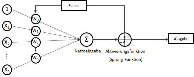
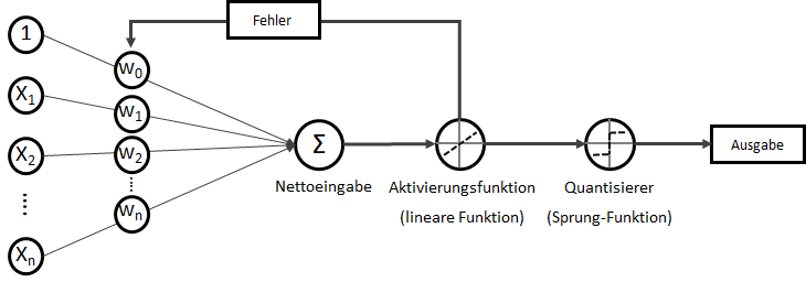
Das Perzeptron (engl. Perceptron) ist ein „Klassiker“ unter den künstlichen neuronalen Netzen. Wenn von einem neuronalen Netz gesprochen wird, ist meistens ein Perzeptron oder eine Variation davon gemeint. Perzeptrons sind mehrschichtige Netze ohne Rückkopplung, mit festen Eingabe- und Ausgabeschichten. Es gibt keine absolut einheitliche Definition eines Perzeptrons, in der Regel ist es jedoch ein reines FeedForward-Netz mit einer Input-Schicht (auch Abtast-Schicht oder Retina genannt) mit statisch oder dynamisch gewichteten Verbindungen zur Ausgabe-Schicht, die (als Single-Layer-Perceptron) aus einem einzigen Neuron besteht. Das eine Neuron setzt sich aus zwei mathematischen Funktionen zusammen: Einer Berechnung der Nettoeingabe und einer Aktivierungsfunktion, die darüber entscheidet, ob die berechnete Nettoeingabe im Brutto nun “feuert” oder nicht. Es ist in seiner Ausgabe folglich binär: Man kann es sich auch als kleines Lämpchen vorstellen, so dass abhängig von den Eingabewerten und den Gewichtungen eine Nettoeingabe (Summe) bildet und eine Sprungfunktion darüber entscheidet, ob am Ende das Lämpchen leuchtet oder nicht. Dieses Konzept der Ausgabeerzeugung wird Forward-Propagation genannt.

Single-Layer-Perceptron

Auch wenn “Netz” für ein einzelnes Perzeptron mit seinem einen Neuron etwas übertrieben wirken mag, ist es doch die Grundlage für viele größere und mehrschichtige Netze.

Betrachten wir nun die Mathematik der Forward-Propagation.

Wir haben eine Menge an Eingabewerten $x_0, x_1 \dots x_n$ . Wobei für $x_0$ als Bias-Input stets gilt: $x_0 = 1,0$ . Der Bias-Input ist nur ein Platzhalter für das wichtige Bias-Gewicht.

$x = \begin{bmatrix} x_0\\ x_1\\ x_2\\ x_3\\ \vdots\\ x_n \end{bmatrix}$

Für jede Eingabevariable wird eine Gewichtsvariable benötigt: $w_0, w_1 \dots w_n$

$w = \begin{bmatrix} w_0\\ w_1\\ w_2\\ w_3\\ \vdots\\ w_n \end{bmatrix}$

Jedes Produkt aus Eingabewert und Gewichtung soll in Summe die Nettoeingabe $z$ bilden. Hier zeigt sich $z$ als lineare mathematische Funktion, die zwei-dimensional leicht als $z = w_0 + w_1 \cdot x_1$ mit $w_0$ als Y-Achsenschnitt wenn $x_1 = 0$ .

$z = w_0 \cdot x_0 + w_1 \cdot x_1 + \dots + w_n \cdot x_n$

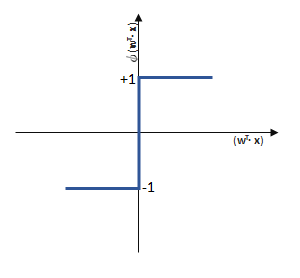
Die lineare Funktion wird nur durch die Sprungfunktion als sogenannte Aktivierungsfunktion zu einer binären Klasseneinteilung (siehe hierzu: Machine Learning – Regression vs Klassifikation), denn wenn $z$ einen festzulegenden Schwellwert $\theta$ überschreitet, liefert die Sprungfunktion $\phi$ mit der Eingabe $z$ einen anderen Wert als wenn dieser Schwellwert nicht überschritten wird.

(1) $\begin{equation*} \phi(z) = \begin{cases} 1 & \text{wenn } z \le \theta \\ -1 & \text{wenn } z < \theta \\ \end{cases} \end{equation*}$

Die Definition dieser Aktivierungsfunktion ist der Kern der Klassifikation und viele erweiterte künstliche neuronale Netze unterscheiden sich im Wesentlichen vom Perzeptron dadurch, dass die Aktivierungsfunktion komplexer ist, als eine reine Sprungfunktion, beispielsweise als Sigmoid-Funktion (basierend auf der logistischen Funktion) oder die Tangens hyperbolicus (tanh) -Funktion. Mehr darüber dann im nächsten Artikel dieser Artikelserie, bleiben wir also bei der einfachen Sprungfunktion.

Künstliche neuronale Netze sind im Grunde nichts anderes als viel-dimensionale, mathematische Funktionen, die durch Schaltung als Neuronen nebeneinander (Neuronen einer Schicht) und hintereinander (mehrere Schichten) eine enorme Komplexität erfassen können. Die Gewichtungen sind dabei die Stellschraube, die die Form der mathematischen Funktion gestaltet, aus Geraden und Kurven, um eine Punktwolke zu beschreiben (Regression) oder um Klassengrenzen zu identifizieren (Klassifikation).

Eine andere Sichtweise auf künstliche neuronale ist die des Filters: Ein künstliches neuronales Netz nimmt alle Eingabe-Variablen entgegen (z. B. alle Pixel eines Bildes) und über ein Training werden die Gewichtungen (die Form des Filters) so gestaltet, dass der Filter immer zu richtigen Klasse (im Kontext der Bildklassifikation: die Objektklasse) führt.

Kommen wir nochmal kurz zurück zu der Berechnung der Nettoeingabe $z$ . Da diese Schreibweise…

$z = w_0 \cdot x_0 + w_1 \cdot x_1 + \dots + w_n \cdot x_n$

… recht anstrengend ist, schreiben Fortgeschrittene der linearen Algebra lieber $z = w^T \cdot x$ .

$z = w^T \cdot x$

Das hochgestellte $T$ steht dabei für transponieren. Transponieren bedeutet, dass Spalten zu Zeilen werden – oder umgekehrt.

Beispielsweise befüllen wir zwei Vektoren $x$ und $w$ mit beispielhaften Inhalten:

Eingabewerte:

$x = \begin{bmatrix} 5\\ 12\\ 30\\ 2 \end{bmatrix}$

Gewichtungen:

$w = \begin{bmatrix} 1\\ 2\\ 5\\ 12 \end{bmatrix}$

Kann nun die Nettoeingabe $z$ berechnet werden, denn der Gewichtungsvektor wird vom Spaltenvektor zum Zeilenvektor. So kann – mathematisch korrekt dargestellt – jedes Element des einen Vektors mit dem zugehörigen Element des anderen Vektors multipliziert werden, die dabei entstehenden Ergebniswerte werden summiert.

$z = w^T \cdot x = \big[1\text{ }2\text{ }5\text{ }12\big] \cdot \begin{bmatrix} 5\\ 12\\ 30\\ 2 \end{bmatrix} = 1 \cdot 5 + 2 \cdot 12 + 5 \cdot 30 + 12 \cdot 2 = 203$

Zurück zur eigentlichen Aufgabe des künstlichen neuronalen Netzes: Klassifikation! (Regression, Clustering und Dimensionsreduktion blenden wir ja in diesem Artikel als Aufgabe aus 🙂

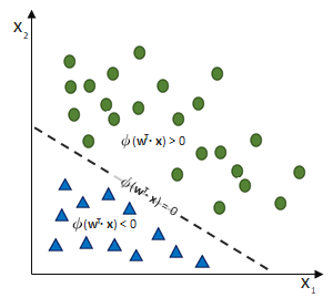
Das Perzeptron soll zwei Klassen trennen. Dafür sollen alle Eingaben richtig gewichtet werden, so dass die entstehende Nettoeingabe $z$ die Sprungfunktion dann aktiviert, wenn der Datensatz nicht für die eine, sondern für die andere Klasse ausweist.

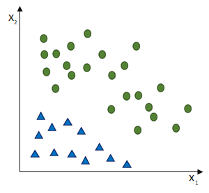
Da wir es mit einer linearen Funktion $z$ zutun haben, ist die Konvergenz (= Passgenauigkeit des Models mit der Realität) eines Single-Layer-Perzeptrons nur für lineare Trennbarkeit möglich!

Training des Perzeptron-Netzes

Die Aufgabe ist nun, die richtigen Gewichte zu finden – und nicht nur irgendwelche richtigen, sondern genau die optimalen. Die Frage, die sich für jedes künstliche neuronale Netz stellt, ist die nach den richtigen Gewichtungen. Das Training eines Perzeptron ist vergleichsweise einfach, gerade weil es binär ist. Denn binär bedeutet auch, dass wenn eine falsche Antwort gegeben wurde, muss das jeweils andere mögliche Ergebnis korrekt sein.

Das Training eines Perzeptrons funktioniert wie folgt:

Setze alle Gewichtungen auf den Wert 0,00
Mit jedem Datensatz des Trainings
1. Berechne den Ausgabewert $\^{y}$
2. Vergleiche den Ausgabewert $\^{y}$ mit dem tatsächlichen Ergebnis $y$
3. Aktualisiere die Gewichtungen entgegen des Fehlers: $w_i = w_i + \Delta w_i$

Wobei die Gewichtsanpassung $\Delta w_i$ entgegen des Fehlers (bzw. hin zur jeweils anderen möglichen Antwort) geschieht:

$\Delta w_i = (\^{y}_j - y_j ) \cdot x_i$

Anmerkung für die Experten: Die Schrittweite $\eta$ blenden wir hier einfach mal aus. Bitte einfach von $\eta = 1.0$ ausgehen.

$\Delta w_i$ ist die Differenz aus der Prädiktion und dem tatsächlichen Ergebnis (Klasse). Alle Gewichtungen werden mit jedem Fehler gleichzeitig aktualisiert. Sind alle Gewichtungen aktualisiert, kommt der nächste Durchlauf (erneuter Vergleich zwischen $\^{y}$ und $y$ ), nicht zu vergessen ist dabei natürlich die Abhängigkeit von den Eingabewerten x:

$\Delta w_0 = (\^{y}_j - y_j ) \cdot x_0$

$\Delta w_2 = (\^{y}_j - y_j ) \cdot x_1$

$\Delta w_2 = (\^{y}_j - y_j) \cdot x_2$

$\Delta w_n = (\^{y}_j - y_j) \cdot x_n$

Training eines Perzeptrons

Das Training im überwachten Lernen basiert immer auf der Idee, den Ausgabe-Fehler (die Differenz zwischen Prädiktion und tatsächlich korrektem Ergebnis) zu betrachten und die Klassifikationslogik an den richtigen Stellschrauben (bei neuronalen Netzen sind das die Gewichtungen) entgegen des Fehlers anzupassen.

Richtige Klassifikations-Situationen können True-Positives und True-Negatives darstellen, die zu keiner Gewichtsanpassung führen sollen:

True-Positive -> Klassifikation: 1 | korrekte Klasse: 1

$\Delta w_i = (\^{y}_j - y_j) \cdot x_i = (1 - 1) \cdot x_i = 0$

True-Negative-> Klassifikation: -1 | korrekte Klasse: -1

$\Delta w_i = (\^{y}_j - y_j) \cdot x_i = (-1 - -1) \cdot x_i = 0$

Falsche Klassifikationen erzeugen einen Fehler, der zu einer Gewichtsanpassung entgegen des Fehlers führen soll:

False-Positive -> Klassifikation: 1 | korrekte Klasse: -1

$\Delta w_i = (\^{y}_j - y_j) \cdot x_i = (1 - -1) \cdot x_i = 2 \cdot x_i$

False-Negative -> Klassifikation: -1 | korrekte Klasse: 1

$\Delta w_i = (\^{y}_j - y_j) \cdot x_i = (-1 - 1) \cdot x_i = -2 \cdot x_i$

Imaginäres Trainingsbeispiel eines Single-Layer-Perzeptrons (SLP)

Nehmen wir an, dass $x_1 = 0,5$ ist und das SLP irrtümlicherweise die Klasse $\^{y_1} = -1$ ausgewiesen hat, obwohl die korrekte Klasse $y_1 = +1$ wäre. (Und die Schrittweite lassen wir bei $\eta = 1,0$ )

Dann passiert folgendes:

$\Delta w_1 = (\^{y}_1 - y_1) \cdot x_1 = (-1 - 1) \cdot 0,5 = -2,0 \cdot 0,5 = -1,0$

Die Gewichtung $w_1$ verringert sich entsprechend $w_1 = w_1 + \Delta w_1 = w_1 - 1,0$ und somit wird die Wahrscheinlichkeit größer, dass wenn bei der nächsten Iteration ( $j=1$ ) wieder die Klasse +1 korrekt sei, den Schwellwert $\phi(z)$ zu unterschreiten und auf eben diese korrekte Klasse zu stoßen.

Die Aktualisierung der Gewichtung $\Delta w_i$ ist proportional zu $x_i$ . So würde beispielsweise ein neues $x_1=2,0$ (bei Iteration $j=2$ ) zu einer irrtümlichen Klassifikation $\^(y_2) = -1$ ( $y_2 = +1$ ) führen, würde die Entscheidungsgrenze zur korrekten Prädiktion der Klasse beim nächsten Durchlauf ( $j = 3$ ) an $w_1$ noch weiter in die gleiche Richtung verschoben werden:

$\Delta w_1 = (\^{y}_2 - y_2) \cdot x_1 = (-1 - 1) \cdot 2,0 = -2,0 \cdot 2,0 = -4,0$

Mehr zum Training von künstlichen neuronalen Netzen ist im nächsten Artikel dieser Artikelserie zu erfahren.

Single-Layer-Perzeptrons (SLP) – Beispiel mit der boolischen Trennung

Verlassen wir nun das Training des Perzeptrons und gehen einfach mal davon aus, dass die idealen Gewichte schon gefunden wurden und schauen uns nun an, was ein Perzeptron alles (nicht) kann. Denn nicht vergessen, es soll eigentlich Klassen unterscheiden bzw. die dafür nötigen Entscheidungsgrenzen finden.

Boolische Operatoren unterscheiden Fälle nach boolischen Werten. Sie sind ein beliebtes “Hello World” für die Einarbeitung in die lineare Entscheidungslogik eines Perzeptrons. Es gibt drei grundlegende boolische Vergleichsoperatoren: AND, OR und XOR

x1	x2	AND	OR	XOR
0	0	0	0	0
0	1	0	1	1
1	0	0	1	1
1	1	1	1	0

Ein Perzeptron zur Lösung dieser Aufgabe bräuchte also zwei Dimensionen (+ Bias): $x_1$ und $x_2$
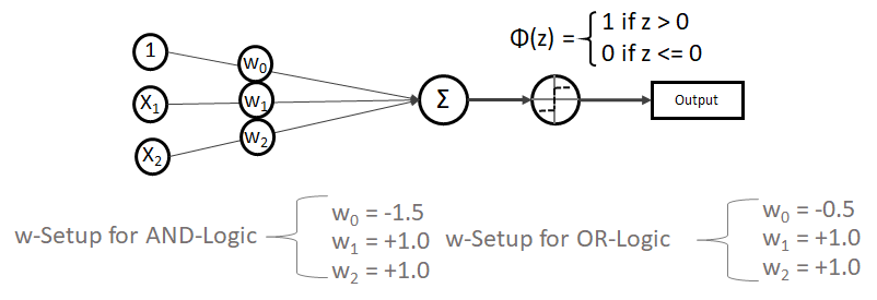
Und es müsste Gewichtungen haben, die dafür sorgen, dass die Vorhersage entsprechend der Logik AND, OR oder XOR mit $\^{y} = \phi(z) = \phi (w_0 \cdot 1 + w_1 \cdot x_1 + w_2 \cdot x_2)$ funktioniert.

Dabei ist es wichtig, dass wir auch phi $\phi$ als Sprungfunktion definieren. Sie könnte beispielsweise so aussehen, dass sie auf den Wert $\phi(z) = 1$ springt, wenn z > 0 ist, ansonsten aber $\phi(z) = 0$ bleibt.

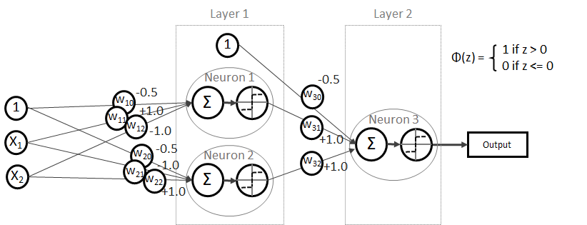
Das Netz und die Gewichtungen (w-Setup) könnten für die AND- und die OR-Logik so aussehen:

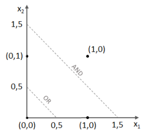
Die Gewichtungen funktionieren beim SLP problemlos, denn wir haben es mit linear trennbaren Problemen zutun:

Kleiner Test gefällig? So nehmen wir uns erstmal die AND-Logik vor:

Wenn x1 = 0 und x2 = 0 ist, gilt: $z = -1,5 \cdot 1 + 1 \cdot 0 + 1 \cdot 0 = - 1,5$ ,
wie erhalten als Prädiktion $\phi(z) = \phi(-1,5) = 0$
Wenn x1 = 1 und x2 = 0 ist, gilt: $z = -1,5 \cdot 1 + 1 \cdot 1 + 1 \cdot 0 = - 0,5$ ,
wie erhalten als Prädiktion $\phi(z) = \phi(-0,5) = 0$
Wenn x1 = 1 und x2 = 1 ist, gilt: $z = -1,5 \cdot 1 + 1 \cdot 1 + 1 \cdot 1 = + 0,5$ ,
wie erhalten als Prädiktion $\phi(z) = \phi(0,5) = 1$

Scheint zu funktionieren!

Und dann die OR-Logik mit

Wenn x1 = 0 und x2 = 0 ist, gilt: $z = -0,5 \cdot 1 + 1 \cdot 0 + 1 \cdot 0 = - 0,5$ ,
wie erhalten als Prädiktion $\phi(z) = \phi(-0,5) = 0$
Wenn x1 = 1 und x2 = 0 ist, gilt: $z = -0,5 \cdot 1 + 1 \cdot 1 + 1 \cdot 0 = + 0,5$ ,
wie erhalten als Prädiktion $\phi(z) = \phi(0,5) = 1$
Wenn x1 = 1 und x2 = 1 ist, gilt: $z = -0,5 \cdot 1 + 1 \cdot 1 + 1 \cdot 1 = + 1,5$ ,
wie erhalten als Prädiktion $\phi(z) = \phi(1,5) = 1$

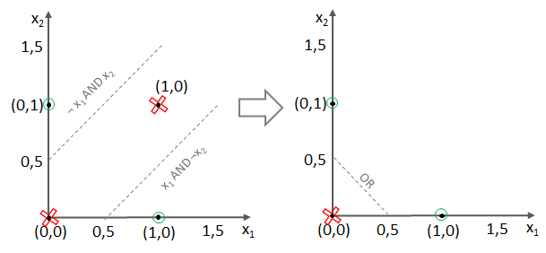
Super! Jedoch stellt sich nun die Frage, wie das XOR-Problem zu lösen ist, denn das bedingt sowohl die Grenzen von AND als auch jene des OR-Operators.

Multi-Layer-Perzeptron (MLP) bzw. (Deep) Feed Forward (FF) Net

Denn ein XOR kann mathematisch auch so korrekt beschrieben werden: $x_1 \text{ xor } x_2 = (x_1 \text{ and } \neg x_2) \text{ or } (\neg x_1 \text{ and } x_2)$

Testen wir es aus!

Wenn x1 = 0 und x2 = 0 ist, gilt:
$z_1 = w_{10} \cdot 1 + w_{11} \cdot x1 + w_{12} \cdot x2 = -0.5 \cdot 1 + 1,0 \cdot 0 - 1,0 \cdot 0 = -0,5$ und somit $\phi(z_1) = \phi(-0,5) = 0$
$z_2 = w_{20} \cdot 1 + w_{21} \cdot x1 + w_{22} \cdot x2 = -0.5 \cdot 1 - 1,0 \cdot 0 + 1,0 \cdot 0 = -0,5$ und somit $\phi(z_2) = \phi(-0,5) = 0$
$z_3 = w_{30} \cdot 1 + w_{31} \cdot \phi(z_1) + w_{32} \cdot \phi(z_2) = -0,5 \cdot 1 + 1,0 \cdot 0 + 1,0 \cdot 0 = -0,5$ und somit $\phi(z_3) = \phi(-0,5) = 0$
Wenn x1 = 1 und x2 = 0 ist, gilt:
$z_1 = w_{10} \cdot 1 + w_{11} \cdot x1 + w_{12} \cdot x2 = -0.5 \cdot 1 + 1,0 \cdot 1 - 1,0 \cdot 0 = 0,5$ und somit $\phi(z_1) = \phi(0,5) = 1$
$z_2 = w_{20} \cdot 1 + w_{21} \cdot x1 + w_{22} \cdot x2 = -0.5 \cdot 1 - 1,0 \cdot 1 + 1,0 \cdot 0 = -1,5$ und somit $\phi(z_2) = \phi(-1,5) = 0$
$z_3 = w_{30} \cdot 1 + w_{31} \cdot \phi(z_1) + w_{32} \cdot \phi(z_2) = -0,5 \cdot 1 + 1,0 \cdot 1 + 1,0 \cdot 0 = 0,5$ und somit $\phi(z_3) = \phi(0,5) = 1$
Wenn x1 = 0 und x2 = 1 ist, gilt:
$z_1 = w_{10} \cdot 1 + w_{11} \cdot x1 + w_{12} \cdot x2 = -0.5 \cdot 1 + 1,0 \cdot 0 - 1,0 \cdot 1 = -1,5$ und somit $\phi(z_1) = \phi(-1,5) = 0$
$z_2 = w_{20} \cdot 1 + w_{21} \cdot x1 + w_{22} \cdot x2 = -0.5 \cdot 1 - 1,0 \cdot 0 + 1,0 \cdot 1 = 0,5$ und somit $\phi(z_2) = \phi(0,5) = 1$
$z_3 = w_{30} \cdot 1 + w_{31} \cdot \phi(z_1) + w_{32} \cdot \phi(z_2) = -0,5 \cdot 1 + 1,0 \cdot 0 + 1,0 \cdot 1 = 0,5$ und somit $\phi(z_3) = \phi(0,5) = 1$
Wenn x1 = 1 und x2 = 1 ist, gilt:
$z_1 = w_{10} \cdot 1 + w_{11} \cdot x1 + w_{12} \cdot x2 = -0.5 \cdot 1 + 1,0 \cdot 1 - 1,0 \cdot 1 = -1,5$ und somit $\phi(z_1) = \phi(-0,5) = 0$
$z_2 = w_{20} \cdot 1 + w_{21} \cdot x1 + w_{22} \cdot x2 = -0.5 \cdot 1 - 1,0 \cdot 1 + 1,0 \cdot 1 = 0,5$ und somit $\phi(z_2) = \phi(-0,5) = 0$
$z_3 = w_{30} \cdot 1 + w_{31} \cdot \phi(z_1) + w_{32} \cdot \phi(z_2) = -0,5 \cdot 1 + 1,0 \cdot 0 + 1,0 \cdot 0 = -0,5$ und somit $\phi(z_3) = \phi(-0,5) = 0$

Es funktioniert!

Mehrfachklassifikation mit dem Perzeptron

Ein Perzeptron-Netz klassifiziert binär, die Ausgabe beschränkt sich auf 1 oder -1 bzw. 0 oder 1.

Jedoch wird in der Praxis oftmals eine One-vs-All (OvA) bzw. One-vs-Rest (OvR) Klassifikation implementiert. In diesem Fall steht die 1 für die Erkennung einer konkreten Klasse, während alle anderen übrigen Klassen als negativ betrachtet werden.

Um jede Klasse erkennen zu können, werden n Klassifizierer (= n Perzeptron-Netze) benötigt. Jedes Perzeptron-Netz ist auf die Erkennung einer bestimmten Klasse trainiert.

Adaline – Oder: die Limitation des Perzeptrons

Das Perzeptron wird nur über eine Sprungfunktion aktiviert. Das schränkt die Feinabstimmung des Trainings enorm ein. Besser sind Aktivierungen über stetige Funktionen, die dann nämlich differenzierbar (ableitbar) sind. Das ergibt eine konvexe Fehlerfunktion mit einem eindeutigen Minimum. Der Adaline-Algorithmus (ADAptive Linear NEuron) erweitert die Idee des Perzeptrons um genau diese Idee. Der wesentliche Fortschritt der Adaline-Regel gegenüber der des Perzeptrons ist demnach, dass die Aktualisierung der Gewichtungen nicht wie beim Perzeptron auf einer einfachen Sprungfunktion, sondern auf einer linearen, stetigen Aktivierungsfunktion beruht.

Single-Layer-Adaline

Wie ein künstliches neuronales Netz mit der Kategorie Adaline trainiert werden kann, wird im nächsten Artikel dieser Artikelserie erläutert.

Weiterführende Netz-Konzepte (CNN und RNN)

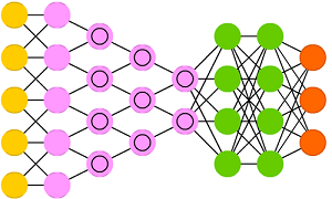
Wer bereits mit Frameworks wie TensorFlow in das Deep Learning eingestiegen ist, hat möglicherweise schon erweiterte Konzepte der künstlichen neuronalen Netze kennen gelernt. Die CNNs (Convolutional Neuronal Network) sind im Moment die Wahl für die Verarbeitung von hochdimensionalen Aufgaben, beispielsweise die Bilderkennung (Computer Vision) und Texterkennung (NLP). Das CNN erweitert die Möglichkeiten mit neuronalen Netzen deutlich, indem ein Netz zur Dimensionsreduktion vorgeschaltet wird, im Kern steckt jedoch weiterhin die Idee der MLPs. Beim Einsatz in der Bilderkennung funktionieren CNNs vereinfacht gesprochen so, dass der vorgeschaltete Netzbereich die Millionen Bildpixel sektorweise ausliest (Convolution, Faltung durch Auslesen über Sektoren, die sich gegenseitig überlappen), verdichtet (Pooling, beispielsweise über nicht-lineare Funktionen wie max()) und dann – nach diesem Prozedere – ähnlich eim MLP klassifiziert.

Eine andere erweiterte Form sind RNNs (Recurrent Neuronal Network), die ebenfalls auf der Idee des MLPs basieren, dieses Konzept jedoch dank Rückverbindungen (Neuronen senden an vorherige Schichten) und Selbstverbindungen (Neuronen senden an sich selbst) wiederum auf den Kopf stellen.

Dennoch ist es für das tiefere Verständnis von CNNs und RNNs essenziell, dass vorher das Konzept des MLPs verstanden ist. Es ist die einfachste Form der auch heute noch am meisten eingesetzten und sehr mächtigen Netz-Topologien.

Im Jahr 2016 hatte Fjodor van Veen von asimovinstitute.org hatte – dankenswerterweise – mal eine Zusammenstellung von Netz-Topologien erstellt, auf die ich heute noch immer mal wieder einen Blick werfe:

Künstliche neuronale Netze – Topologie-Übersicht von Fjodor van Veen

Buchempfehlungen

Die folgenden Bücher nutze ich für mein Selbststudium von Machine Learning und Deep Learning und sind teilweise Gedankenvorlagen auch für diesen Artikel gewesen:


Machine Learning mit Python und Scikit-Learn und TensorFlow: Das umfassende Praxis-Handbuch für Data Science, Predictive Analytics und Deep Learning (mitp Professional)	Deep Learning mit Python und Keras: Das Praxis-Handbuch vom Entwickler der Keras-Bibliothek(mitp Professional)

Tag Archive for: Linear Algebra

Understanding Linear Regression with all Statistical Terms

Why do we use Regression Analysis?

What is Linear Regression?

Application of Linear Regression:

Real-world examples of linear regression models

Assumptions of Linear Regression:

Rethinking linear algebra part two: ellipsoids in data science

1 Our expedition of eigenvectors still continues

2 Rotation or projection?

3 Types of quadratic curves.

4 Eigenvectors are gradients and sometimes variances.

5 Ellipsoids in Gaussian distributions.

Appendix: making a model of a bunch of grape with ellipsoid berries.

The algorithm known as PCA and my taxonomy of linear dimension reductions

1. My taxonomy on linear dimension reduction

2. PCA

3. Fitting orthogonal axes on data

4. Practical three dimensional example of PCA

Appendix: Playing with my toy PCA on MNIST dataset

Funktionsweise künstlicher neuronaler Netze

Perzeptron

Training des Perzeptron-Netzes

Training eines Perzeptrons

Imaginäres Trainingsbeispiel eines Single-Layer-Perzeptrons (SLP)

Single-Layer-Perzeptrons (SLP) – Beispiel mit der boolischen Trennung

Multi-Layer-Perzeptron (MLP) bzw. (Deep) Feed Forward (FF) Net

Mehrfachklassifikation mit dem Perzeptron

Adaline – Oder: die Limitation des Perzeptrons

Weiterführende Netz-Konzepte (CNN und RNN)

Buchempfehlungen

Interesting links

Pages

Categories

Archive