Rethinking linear algebra part two: ellipsoids in data science
*This is the fourth article of my article series “Illustrative introductions on dimension reduction.”
1 Our expedition of eigenvectors still continues
This article is still going to be about eigenvectors and PCA, and this article still will not cover LDA (linear discriminant analysis). Hereby I would like you to have more organic links of the data science ideas with eigenvectors.
In the second article, we have covered the following points:
- You can visualize linear transformations with matrices by calculating displacement vectors, and they usually look like vectors swirling.
- Diagonalization is finding a direction in which the displacement vectors do not swirl, and that is equal to finding new axis/basis where you can describe its linear transformations more straightforwardly. But we have to consider diagonalizability of the matrices.
- In linear dimension reduction such as PCA or LDA, we mainly use types of matrices called positive definite or positive semidefinite matrices.
In the last article we have seen the following points:
- PCA is an algorithm of calculating orthogonal axes along which data “swell” the most.
- PCA is equivalent to calculating a new orthonormal basis for the data where the covariance between components is zero.
- You can reduced the dimension of the data in the new coordinate system by ignoring the axes corresponding to small eigenvalues.
- Covariance matrices enable linear transformation of rotation and expansion and contraction of vectors.
I emphasized that the axes are more important than the surface of the high dimensional ellipsoids, but in this article let’s focus more on the surface of ellipsoids, or I would rather say general quadratic curves. After also seeing how to draw ellipsoids on data, you would see the following points about PCA or eigenvectors.
- Covariance matrices are real symmetric matrices, and also they are positive semidefinite. That means you can always diagonalize covariance matrices, and their eigenvalues are all equal or greater than 0.
- PCA is equivalent to finding axes of quadratic curves in which gradients are biggest. The values of quadratic curves increases the most in those directions, and that means the directions describe great deal of information of data distribution.
- Intuitively dimension reduction by PCA is equal to fitting a high dimensional ellipsoid on data and cutting off the axes corresponding to small eigenvalues.
Even if you already understand PCA to some extent, I hope this article provides you with deeper insight into PCA, and at least after reading this article, I think you would be more or less able to visually control eigenvectors and ellipsoids with the Numpy and Maplotlib libraries.
*Let me first introduce some mathematical facts and how I denote them throughout this article in advance. If you are allergic to mathematics, take it easy or please go back to my former articles.
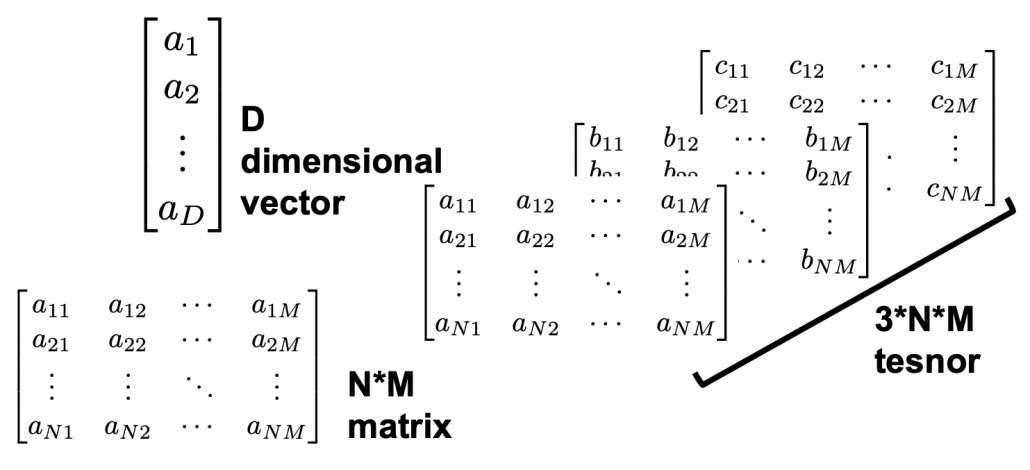
- Any quadratic curves can be denoted as
 , where


 .
. - When I want to clarify dimensions of variables of quadratic curves, I denote parameters as
 .
. - If a matrix
 is a real symmetric matrix, there exist a rotation matrix
  such that
  , where
  and
and  .
.  are eigenvectors corresponding to
  respectively.
 - PCA corresponds to a case of diagonalizing where is a covariance matrix of certain data. When I want to clarify that is a covariance matrix, I denote it as
 .
. - Importantly covariance matrices
 are positive semidefinite and real symmetric, which means you can always diagonalize and any of their engenvalues cannot be lower than 0.
*In the last article, I denoted the covariance of data as  , based on Pattern Recognition and Machine Learning by C. M. Bishop.
*Sooner or later you are going to see that I am explaining basically the same ideas from different points of view, using the topic of PCA. However I believe they are all important when you learn linear algebra for data science of machine learning. Even you have not learnt linear algebra or if you have to teach linear algebra, I recommend you to first take a review on the idea of diagonalization, like the second article. And you should be conscious that, in the context of machine learning or data science, only a very limited type of matrices are important, which I have been explaining throughout this article.
2 Rotation or projection?
In this section I am going to talk about basic stuff found in most textbooks on linear algebra. In the last article, I mentioned that if is a real symmetric matrix, you can diagonalize with a rotation matrix  , such that

 , where
  . I also explained that PCA is a case where , that is, is the covariance matrix of certain data. is known to be positive semidefinite and real symmetric. Thus you can always diagonalize and any of their engenvalues cannot be lower than 0.
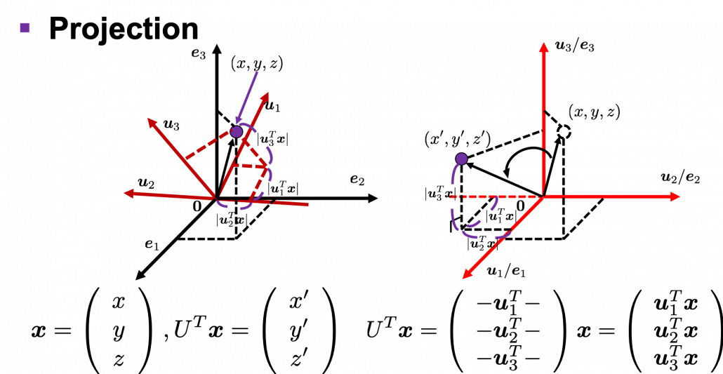
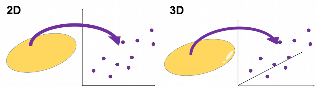
I think we first need to clarify the difference of rotation and projection. In order to visualize the ideas, let’s consider a case of  . Assume that you have got an orthonormal rotation matrix
  which diagonalizes . In the last article I said diagonalization is equivalent to finding new orthogonal axes formed by eigenvectors, and in the case of this section you got new orthonoramal basis
  which are in red in the figure below. Projecting a point
  on the new orthonormal basis is simple: you just have to multiply
  with
with  . Let
. Let  be
be  , and then
  . You can see
  are projected on
  respectively, and the left side of the figure below shows the idea. When you replace the orginal orthonormal basis
  with as in the right side of the figure below, you can comprehend the projection as a rotation from
  to
to  by a rotation matrix .
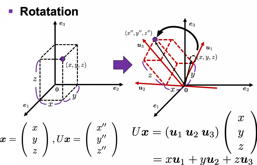
Next, let’s see what rotation is. In case of rotation, you should imagine that you rotate the point in the same coordinate system, rather than projecting to other coordinate system. You can rotate by multiplying it with . This rotation looks like the figure below.
In the initial position, the edges of the cube are aligned with the three orthogonal black axes  , with one corner of the cube located at the origin point of those axes. The purple dot denotes the corner of the cube directly opposite the origin corner. The cube is rotated in three dimensions, with the origin corner staying fixed in place. After the rotation with a pivot at the origin, the edges of the cube are now aligned with a new set of orthogonal axes
  , shown in red. You might understand that more clearly with an equation:
 . In short this rotation means you keep relative position of , I mean its coordinates , in the new orthonormal basis. In this article, let me call this a “cube rotation.”
The discussion above can be generalized to spaces with dimensions higher than 3. When  is an orthonormal matrix and a vector
  , you can project to
  or rotate it to
  , where
  and
and  . In other words
  , which means you can rotate back
  to the original point with the rotation matrix .
I think you at least saw that rotation and projection are basically the same, and that is only a matter of how you look at the coordinate systems. But I would say the idea of projection is more important through out this article.
Let’s consider a function  , where
  is a real symmetric matrix. The distribution of
  is quadratic curves whose center point covers the origin, and it is known that you can express this distribution in a much simpler way using eigenvectors. When you project this function on eigenvectors of , that is when you substitute
  for , you get


 . You can always diagonalize real symmetric matrices, so the formula implies that the shapes of quadratic curves largely depend on eigenvectors. We are going to see this in detail in the next section.
* denotes an inner product of and
  .
.
*We are going to see details of the shapes of quadratic “curves” or “functions” in the next section.
To be exact, you cannot naively multiply or for rotation. Let’s take a part of data I showed in the last article as an example. In the figure below, I projected data on the basis .
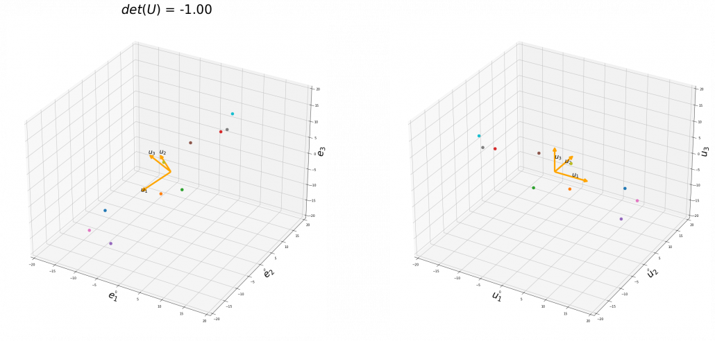
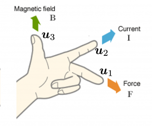
You might have noticed that you cannot do a “cube rotation” in this case. If you make the coordinate system with your left hand, like you might have done in science classes in school to learn Fleming’s rule, you would soon realize that the coordinate systems in the figure above do not match. You need to flip the direction of one axis to match them.
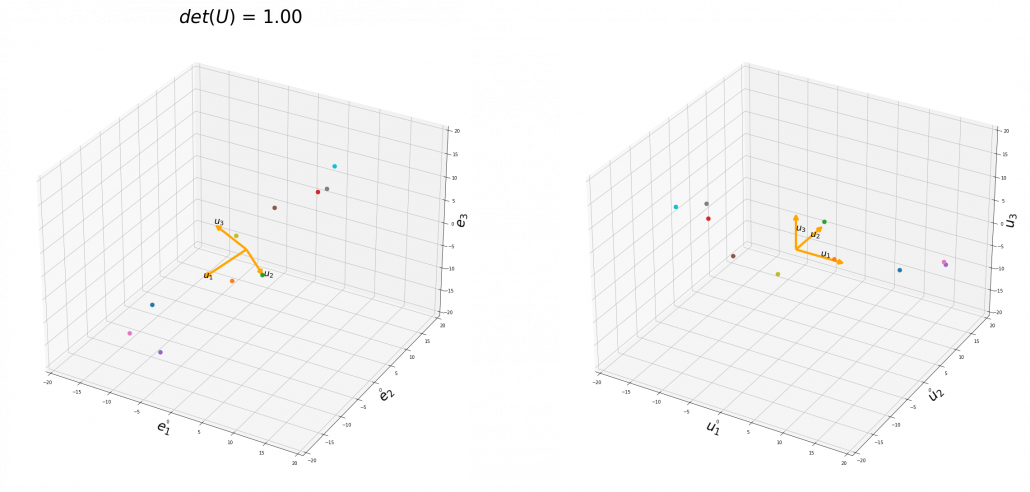
Mathematically, you have to consider the determinant of the rotation matrix . You can do a “cube rotation” when  , and in the case above
  was
was  , and you needed to flip one axis to make the determinant
  . In the example in the figure below, you can match the basis. This also can be generalized to higher dimensions, but that is also beyond the scope of this article series. If you are really interested, you should prepare some coffee and snacks and textbooks on linear algebra, and some weekends.
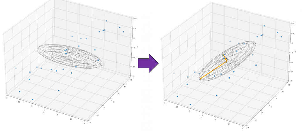
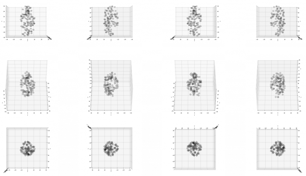
When you want to make general ellipsoids in a 3d space on Matplotlib, you can take advantage of rotation matrices. You first make a simple ellipsoid symmetric about xyz axis using polar coordinates, and you can rotate the whole ellipsoid with rotation matrices. I made some simple modules for drawing ellipsoid. If you put in a rotation matrix which diagonalize the covariance matrix of data and a list of three radiuses  , you can rotate the original ellipsoid so that it fits the data well.
3 Types of quadratic curves.
*This article might look like a mathematical writing, but I would say this is more about computer science. Please tolerate some inaccuracy in terms of mathematics. I gave priority to visualizing necessary mathematical ideas in my article series. If you are not sure about details, please let me know.
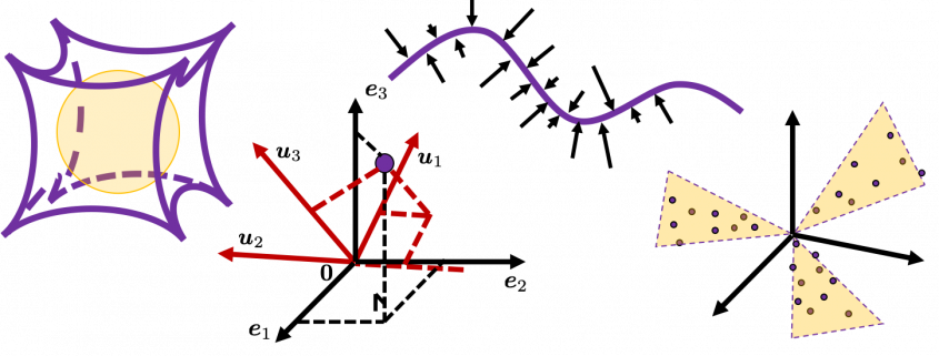
In linear dimension reduction, or at least in this article series you mainly have to consider ellipsoids. However ellipsoids are just one type of quadratic curves. In the last article, I mentioned that when the center of a D dimensional ellipsoid is the origin point of a normal coordinate system, the formula of the surface of the ellipsoid is as follows:  , where satisfies certain conditions. To be concrete, when is the surface of a ellipsoid, has to be diagonalizable and positive definite.
*Real symmetric matrices are diagonalizable, and positive definite matrices have only positive eigenvalues. Covariance matrices , whose displacement vectors I visualized in the last two articles, are known to be symmetric real matrices and positive semi-defintie. However, the surface of an ellipsoid which fit the data is  , not
, not  .
.
*You have to keep it in mind that are all deviations.
*You do not have to think too much about what the “semi” of the term “positive semi-definite” means fow now.
As you could imagine, this is just one simple case of richer variety of graphs. Let’s consider a 3-dimensional space. Any quadratic curves in this space can be denoted as  , where at least one of
  is not
  . Let be
  , then the quadratic curves can be simply denoted with a
  matrix and a 3-dimensional vector
  as follows: , where
  ,
,  . General quadratic curves are roughly classified into the 9 types below.
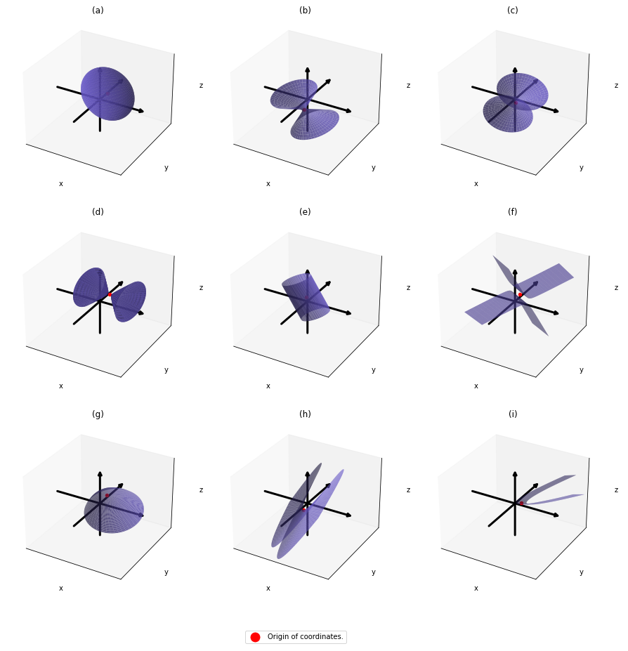
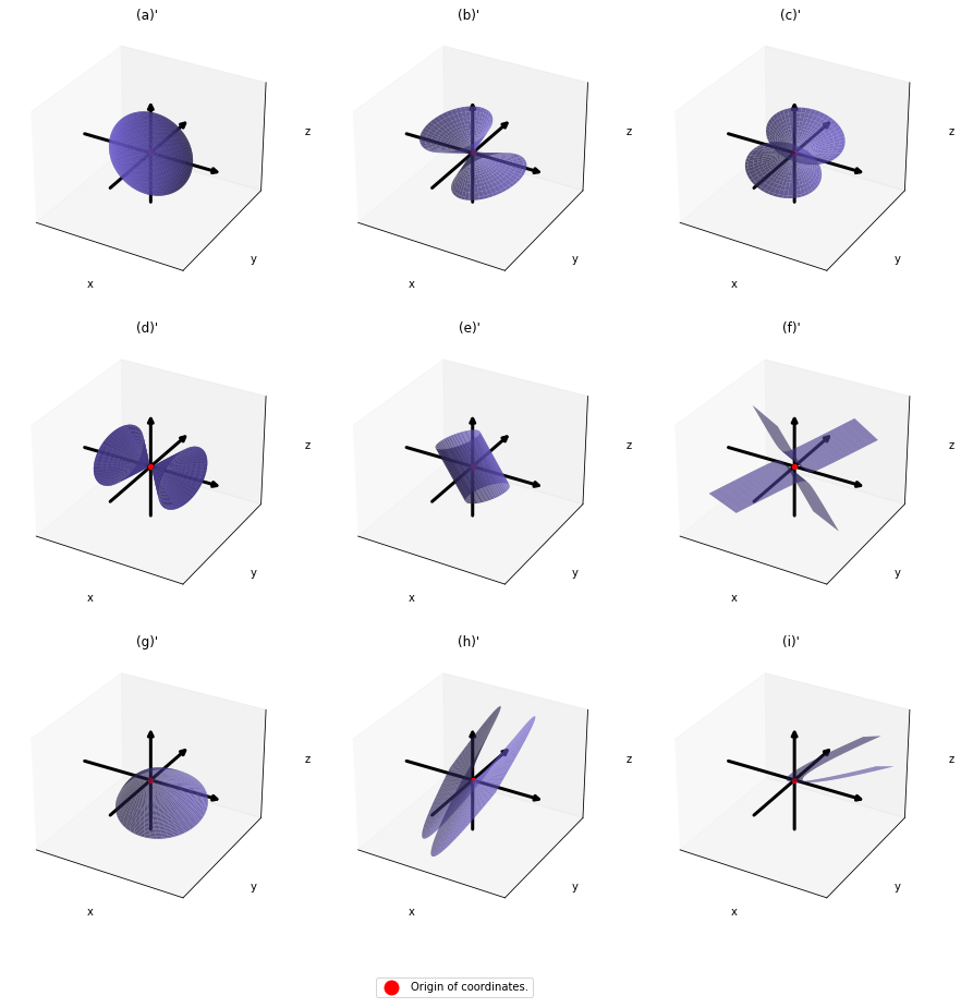
You can shift these quadratic curves so that their center points come to the origin, without rotation, and the resulting curves are as follows. The curves can be all denoted as  .
.
As you can see, is a real symmetric matrix. As I have mentioned repeatedly, when all the elements of a  symmetric matrix are real values and its eigen values are
  , there exist orthogonal/orthonormal matrices such that
  , where . Hence, you can diagonalize the with an orthogonal matrix . Let be an orthogonal matrix such that
 . After you apply rotation by to the curves (a)” ~ (i)”, those curves are symmetrically placed about the xyz axes, and their center points still cross the origin. The resulting curves look like below. Or rather I should say you projected (a)’ ~ (i)’ on their eigenvectors.
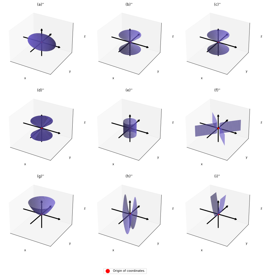
In this article mainly (a)” , (g)”, (h)”, and (i)” are important. General equations for the curves is as follows
- (a)”:

- (g)”:

- (h)”:

- (i)”:

, where  .
.
Even if this section has been puzzling to you, you just have to keep one point in your mind: we have been discussing general quadratic curves, but in PCA, you only need to consider a case where is a covariance matrix, that is . PCA corresponds to the case where you shift and rotate the curve (a) into (a)”. Subtracting the mean of data from each point of data corresponds to shifting quadratic curve (a) to (a)’. Calculating eigenvectors of corresponds to calculating a rotation matrix such that the curve (a)’ comes to (a)” after applying the rotation, or projecting curves on eigenvectors of . Importantly we are only discussing the covariance of certain data, not the distribution of the data itself.
*Just in case you are interested in a little more mathematical sides: it is known that if you rotate all the points on the curve with the rotation matrix  , those points are mapped into a new quadratic curve
  . That means the rotation of the original quadratic curve with (or rather rotating axes) enables getting rid of the terms
  . Also it is known that when
  , with proper translations and rotations, the quadratic curve can be mapped into one of the types of quadratic curves in the figure below, depending on coefficients of the original quadratic curve. And the discussion so far can be generalized to higher dimensional spaces, but that is beyond the scope of this article series. Please consult decent textbooks on linear algebra around you for further details.
4 Eigenvectors are gradients and sometimes variances.
In the second section I explained that you can express quadratic functions  in a very simple way by projecting on eigenvectors of .
You can comprehend what I have explained in another way: eigenvectors, to be exact eigenvectors of real symmetric matrices , are gradients. And in case of PCA, I mean when eigenvalues are also variances. Before explaining what that means, let me explain a little of the totally common facts on mathematics. If you have variables , I think you can comprehend functions  in two ways. One is a normal “functions”
  , and the others are “curves”
  . “Functions” get an input and gives out an output , just as well as normal functions you would imagine. “Curves” are rather sets of such that .
*Please assume that the terms “functions” and “curves” are my original words. I use them just in case I fail to use functions and curves properly.
The quadratic curves in the figure above are all “curves” in my term, which can be denoted as  or
or  . However if you replace
  of (g)”, (h)”, and (i)” with
  , you can interpret the “curves” as “functions” which are denoted as
  . This might sounds too obvious to you, and my point is you can visualize how values of “functions” change only when the inputs are 2 dimensional.
When a symmetric  real matrices
  have two eigenvalues
  , the distribution of quadratic curves can be roughly classified to the following three types.
- (g): Both
 and
and  are positive or negative.
 - (h): Either of or is positive and the other is negative.
- (i): Either of or is 0 and the other is not.
The equations of (g)” , (h)”, and (i)” correspond to each type of  , and thier curves look like the three graphs below.
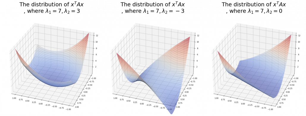
And in fact, when start from the origin and go in the direction of an eigenvector  ,
,  is the gradient of the direction. You can see that more clearly when you restrict the distribution of to a unit circle. Like in the figure below, in case
  , which is classified to (g), the distribution looks like the left side, and if you restrict the distribution in the unit circle, the distribution looks like a bowl like the middle and the right side. When you move in the direction of
  , you can climb the bowl as as high as , in
  as high as .
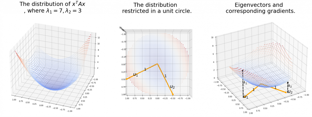
Also in case of (h), the same facts hold. But in this case, you can also descend the curve.
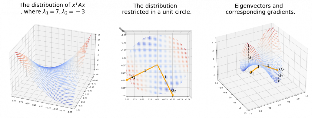
*You might have seen the curve above in the context of optimization with stochastic gradient descent. The origin of the curve above is a notorious saddle point, where gradients are all in any directions but not a local maximum or minimum. Points can be stuck in this point during optimization.
Especially in case of PCA, is a covariance matrix, thus . Eigenvalues of are all equal to or greater than . And it is known that in this case is the variance of data projected on its corresponding eigenvector  . Hence, if you project
  , quadratic curves formed by a covariance matrix , on eigenvectors of , you get
 . This shows that you can re-weight
  , the coordinates of data projected projected on eigenvectors of , with , which are variances . As I mentioned in an example of data of exam scores in the last article, the bigger a variance is, the more the feature described by vary from sample to sample. In other words, you can ignore eigenvectors corresponding to small eigenvalues.
That is a great hint why principal components corresponding to large eigenvectors contain much information of the data distribution. And you can also interpret PCA as a “climbing” a bowl of  , as I have visualized in the case of (g) type curve in the figure above.
*But as I have repeatedly mentioned, ellipsoid which fit data well is

 .
.
*You have to be careful that even if you slice a type (h) curve with a place  the resulting cross section does not fit the original data well because the equation of the cross section is
  The figure below is an example of slicing the same as the one above with
  , and the resulting cross section.
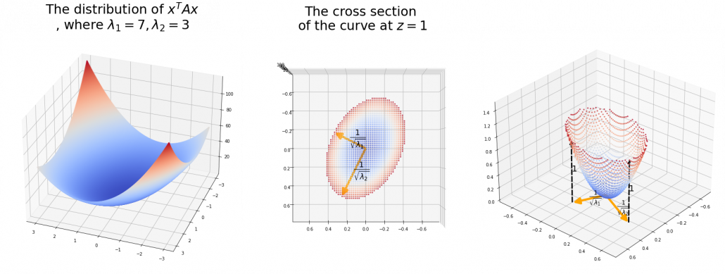
As we have seen, , the eigenvalues of the covariance matrix of data are variances or data when projected on it eigenvectors. At the same time, when you fit an ellipsoid on the data,  is the radius of the ellipsoid corresponding to . Thus ignoring data projected on eigenvectors corresponding to small eigenvalues is equivalent to cutting of the axes of the ellipsoid with small radiusses.
I have explained PCA in three different ways over three articles.
- The second article: I focused on what kind of linear transformations convariance matrices enable, by visualizing displacement vectors. And those vectors look like swirling and extending into directions of eigenvectors of .
- The third article: We directly found directions where certain data distribution “swell” the most, to find that data swell the most in directions of eigenvectors.
- In this article, we have seen PCA corresponds to only one case of quadratic functions, where the matrix is a covariance matrix. When you go in the directions of eigenvectors corresponding to big eigenvalues, the quadratic function increases the most. Also that means data samples have bigger variances when projected on the eigenvectors. Thus you can cut off eigenvectors corresponding to small eigenvectors because they retain little information about data, and that is equivalent to fitting an ellipsoid on data and cutting off axes with small radiuses.
*Let be a covariance matrix, and you can diagonalize it with an orthogonal matrix as follow:  , where . Thus
  . is a rotation, and multiplying a with
  means you multiply each eigenvalue to each element of . At the end enables the reverse rotation.
If you get data like the left side of the figure below, most explanation on PCA would just fit an oval on this data distribution. However after reading this articles series so far, you would have learned to see PCA from different viewpoints like at the right side of the figure below.
5 Ellipsoids in Gaussian distributions.
I have explained that if the covariance of a data distribution is  , the ellipsoid which fits the distribution the best is
  . You might have seen the part
 somewhere else. It is the exponent of general Gaussian distributions:
 . It is known that the eigenvalues of
  are
are  , and eigenvectors corresponding to each eigenvalue are also
  respectively. Hence just as well as what we have seen, if you project
  on each eigenvector of , we can convert the exponent of the Gaussian distribution.
Let  be and
  be
be  , where
  . Just as we have seen,


 . Hence
 .
.
*To be mathematically exact about changing variants of normal distributions, you have to consider for example Jacobian matrices.
This results above demonstrate that, by projecting data on the eigenvectors of its covariance matrix, you can factorize the original multi-dimensional Gaussian distribution into a product of Gaussian distributions which are irrelevant to each other. However, at the same time, that is the potential limit of approximating data with PCA. This idea is going to be more important when you think about more probabilistic ways to handle PCA, which is more robust to lack of data.
I have explained PCA over 3 articles from various viewpoints. If you have been patient enough to read my article series, I think you have gained some deeper insight into not only PCA, but also linear algebra, and that should be helpful when you learn or teach data science. I hope my codes also help you. In fact these are not the only topics about PCA. There are a lot of important PCA-like algorithms.
In fact our expedition of ellipsoids, or PCA still continues, just as Star Wars series still continues. Especially if I have to explain an algorithm named probabilistic PCA, I need to explain the “Bayesian world” of machine learning. Most machine learning algorithms covered by major introductory textbooks tend to be too deterministic and dependent on the size of data. Many of those algorithms have another “parallel world,” where you can handle inaccuracy in better ways. I hope I can also write about them, and I might prepare another trilogy for such PCA. But I will not disappoint you, like “The Phantom Menace.”
Appendix: making a model of a bunch of grape with ellipsoid berries.
If you can control quadratic curves, reshaping and rotating them, you can make a model of a grape of olive bunch on Matplotlib. I made a program of making a model of a bunch of berries on Matplotlib using the module to draw ellipsoids which I introduced earlier. You can check the codes in this page.
*I have no idea how many people on this earth are in need of making such models.

I made some modules so that you can see the grape bunch from several angles. This might look very simple to you, but the locations of berries are organized carefully so that it looks like they are placed around a stem and that the berries are not too close to each other.
The programming code I created for this article is completly available here.
[Refereces]
[1]C. M. Bishop, “Pattern Recognition and Machine Learning,” (2006), Springer, pp. 78-83, 559-577
[2]「理工系新課程 線形代数 基礎から応用まで」, 培風館、(2017)
[3]「これなら分かる 最適化数学 基礎原理から計算手法まで」, 金谷健一著、共立出版, (2019), pp. 17-49
[4]「これなら分かる 応用数学教室 最小二乗法からウェーブレットまで」, 金谷健一著、共立出版, (2019), pp.165-208
[5] 「サボテンパイソン 」
https://sabopy.com/

 matrix, the formula of a D-dimensional ellipsoid whose center is identical to the origin point is as follows:
  , where
  . As is always the case with formulas in data science, you can visualize such ellipsoids if you are talking about 1, 2, or 3 dimensional data like in the figure below, but in general D-dimensional space, it is theoretical/imaginary stuff on blackboards.
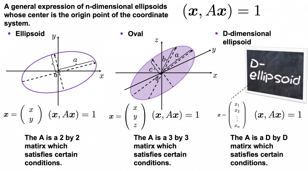
 , where
  or
or  , where
  . These are special cases of the equation
  . In this case the axes of ellipsoids the same as those of the coordinate system. Thus in this simple case,
  or
or  .
. as below (The samples are plotted in purple). Intuitively, the data “swell” the most along the vector
  expresses the data in a better way, and you you can get new coordinate points of the samples by projecting them on new axes as done with yellow lines below.
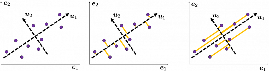
 as below, the data “swell” the most also along
  .
.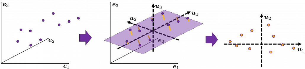
 on the axis
  .
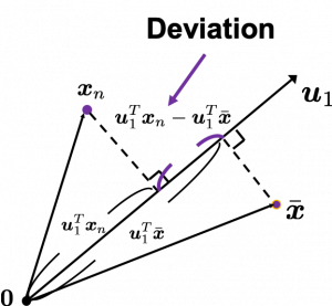
. is the mean of data in the original coordinate, then the deviation of
  on the axis
  , as shown in the figure. Hence the variance, I mean the mean of the deviation on is
  , where
  is the total number of data points. After some deformations, you get the next equation
  , where
  .
.  , and for mathematical derivation we need some college level calculus, so if that is too much for you, you can skip reading this part till the next section.
 . Introducing a
  . In conclusion
  satisfies
  . If you have read my last article on eigenvectors, you wold soon realize that this is an equation for calculating eigenvectors, and that means
  . We have seen that
  is a the variance of data when projected on a vector
 , and in fact the matrix is just a constant multiplication of this covariance matrix. I think now you understand that PCA is calculating the orthogonal eigenvectors of covariance matrix of data, that is diagonalizing covariance matrix with orthonormal eigenvectors. Hence we can guess that covariance matrix enables a type of linear transformation of rotation and expansion and contraction of vectors. And data points swell along eigenvectors of such matrix.
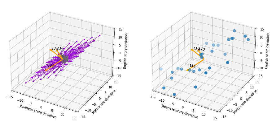
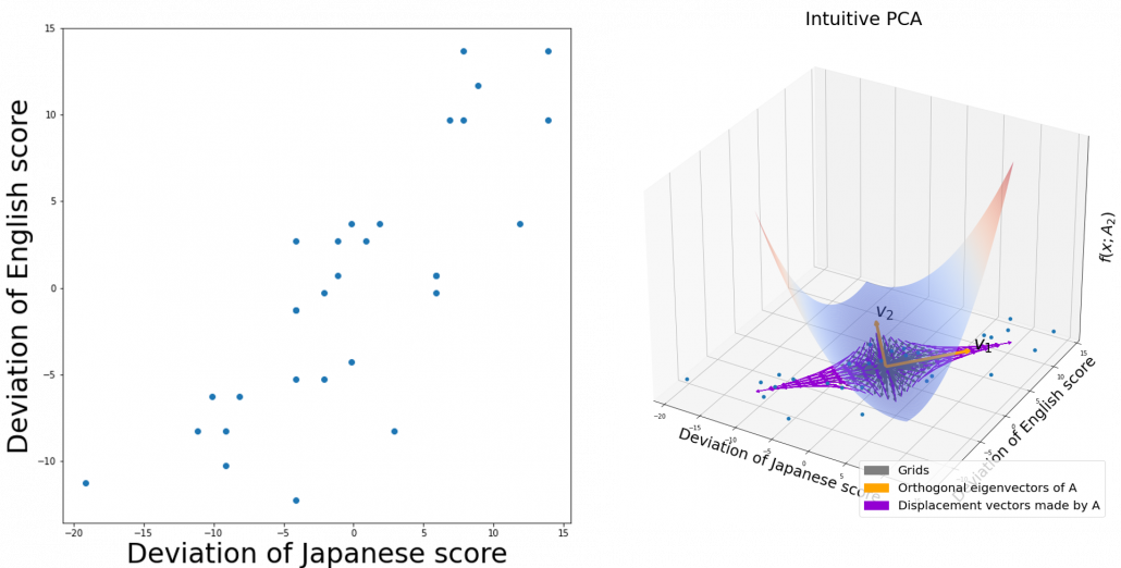
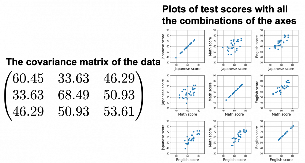
 denote Japanese, Math, English scores respectively. The mean of the data is
  , and the covariance matrix of data in the original coordinate system is
  . The eigenvalues of
  are
are  , and
, and  , and their corresponding unit eigenvectors are
  respectively.
  is an orthonormal matrix, where
  . As I explained in the last article, you can diagonalize
  .
. .
. , and
, and  ).
).  enables a rotation of a rigid body, which means the shape or arrangement of data will not change after the rotation, and
  , and
, and  is the coordinate of
  denotes the coordinate point of the purple point in the red coordinate system.
  denotes the coordinates of data projected on new axes
 , which means you can express deviations of the original data as linear combinations of the three factors
  , and
, and  . We expect that those three factors contain keys for understanding the original data more efficiently. If you concretely write down all the equations for the factors:
  ,
,  , and
, and  . If you examine the coefficients of the deviations
  , and
, and  , we can observe that
  almost equally reflects the deviation of the scores of all the subjects, thus we can say
  is
is  . You can see
  . The variance of data projected on new D-dimensional coordinate system is


 . This means that in the new coordinate system after PCA, covariances between any pair of variants are all zero.
 .
. . Then it mathematically clearer that we can express the data with two factors: “how smart the student is” and “whether he is at scientific side or liberal art side.”
 is called the contribution ratio of eigenvector
  and
and  are respectively
  ,
,  ,
,  . You can decide how many degrees of dimensions you reduce based on this information.

 be a vector space and let
  be a mapping of
  into itself, defined as
  , where
  is
is  dimensional vector. An element
  is called an eigen vector if there exists a number
  such that
  and
and  . In this case
  , belonging to
  . If
. If  is basis of the vector space
  , whose column vectors are eigen vectors
  , where
  .
. Most textbooks keep explaining these type of stuff, but I have to say they lack efforts to make it understandable to readers with low mathematical literacy like me. Especially if you have to apply the idea to data science field, I believe you need more visual understanding of diagonalization. Therefore instead of just explaining the definitions and theorems, I would like to take a different approach. But in order to understand them in more intuitive ways, we first have to rethink waht linear transformation
  means in more visible ways.
 is a vector transformed by
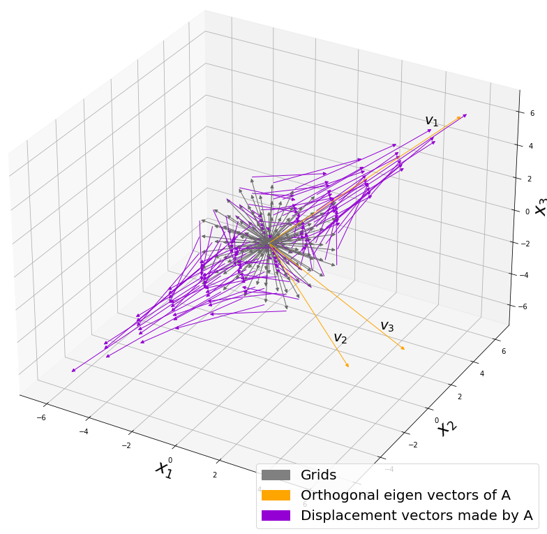
 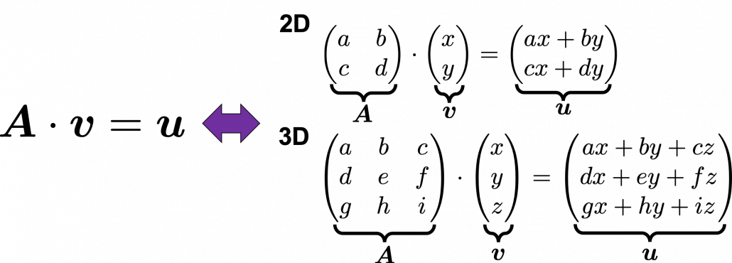 *I am not going to use the term “linear transformation” in a precise way in the context of linear algebra. In this article or in the context of data science or machine learning, “linear transformation” for the most part means products of matrices or vectors.
 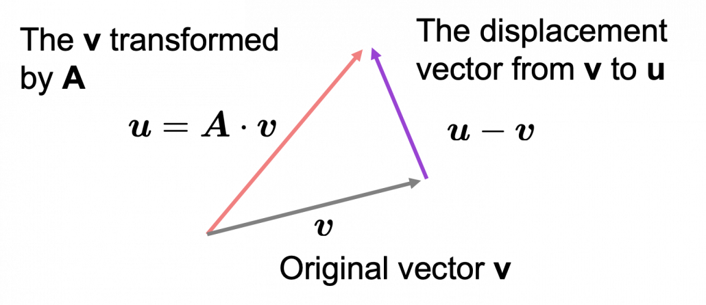 Let’s calculate the displacement vector with more vectors
  , and I prepared several grid vectors
  , which are in purple.
 square matrices
  , and I plotted displace vectors made by the matrices respectively in the figure below.
 , the matrix does not have any real eigan values.
 is classified to, and I am going to explain positive semidefinite matrices in the fourth section.
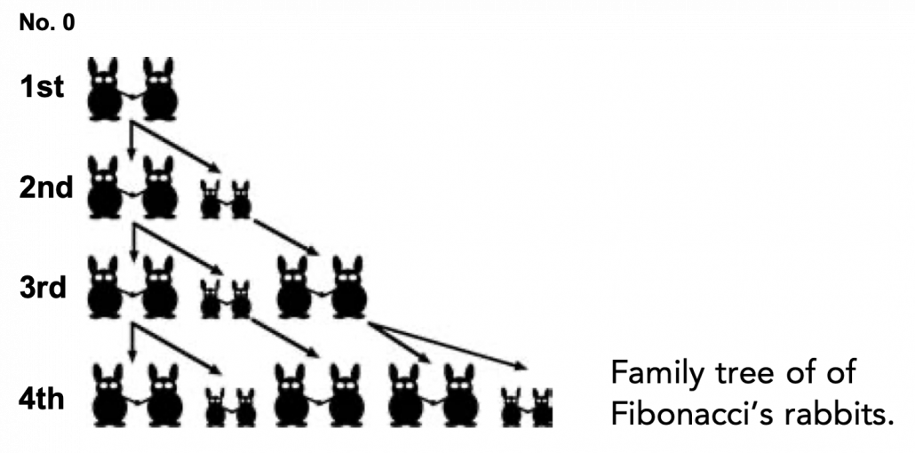
 be the number of pairs of grown up rabbits in the
  generation. One pair of grown up rabbits produce one pair of young rabbit The concrete values of
  are
are  ,
,  ,
,  ,
,  ,
,  ,
,  ,
,  ,
,  . Assume that
  and that
  , then you can calculate the number of the pairs of grown up rabbits in the next generation with the following recurrence relation.
  .Let
.Let  be
be  , then the recurrence relation can be written as
  , and the transition of
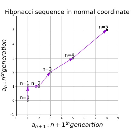
 are eigen values of
  scalars such that
  . According to the definition of eigen values and eigen vectors belonging to them, the following two equations hold:
  . If you calculate
  is, using eigen vectors of
  . In the same way,
  , and
, and  . These equations show that in coordinate system made by eigen vectors of
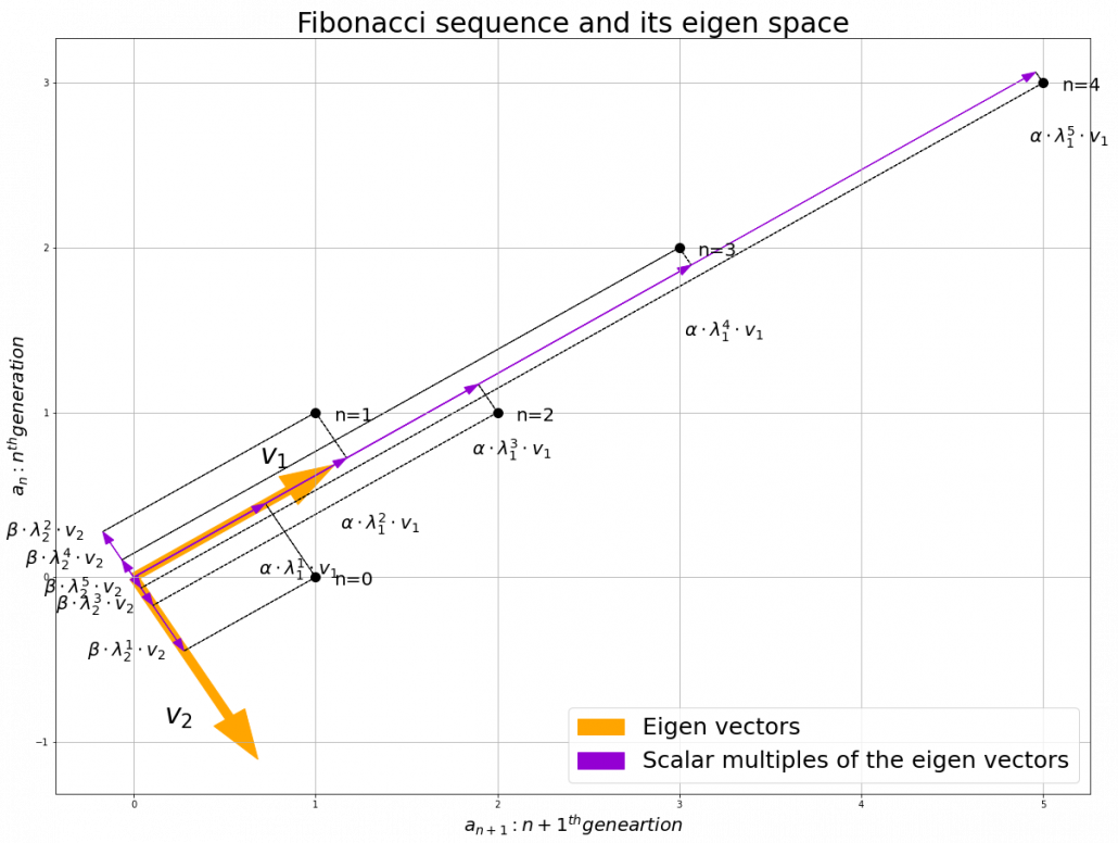
 for all values of the vector
  for all the eigen values
  .
. for all values of the vector
  square positive semidefinite matrix
  , whose linear transformation I visualized the second section, is also positive semidefinite.
 .
.
 , where
  . In other words column vectors
  form an orthonormal coordinate system.
 . Combining this fact with what I have told you so far, you we can reach one conclusion: you can orthogonalize a real symmetric matrix
  is also orthonormal. In other words, assume
  ,
,  also forms a orthonormal coordinate system.
 expands or contracts vectors along each axis. I am going to explain that more precisely in the upcoming articles.
 plotted against parameter
  out of 12 parameters.
 grids respectively in 1, 2, 3 dimensional spaces, the number of the small regions in the grids are respectively 10, 100, 1000. Even though you cannot visualize it anymore, you can make grids for more than 3 dimensional data. If you continue increasing the degree of dimension, the number of grids increases exponentially, and that can soon surpass the number of training data points. That means there would be a lot of empty spaces in such high dimensional grids. And the classifying method above: coloring each grid and classifying unknown samples depending on the colors of the grids, does not work out anymore because there would be a lot of empty grids.
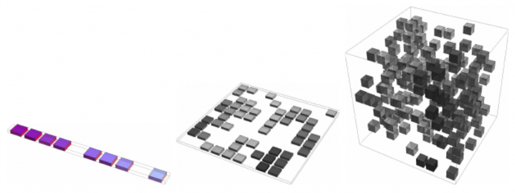
 , where
  is the center point and
  is length of radius. When
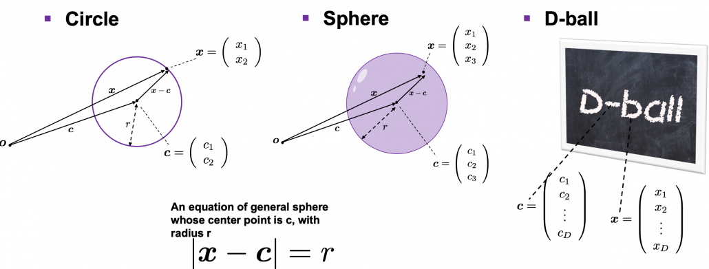
 , and that in each cube is
  .
. 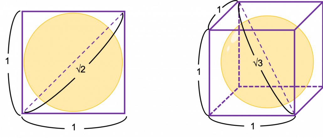
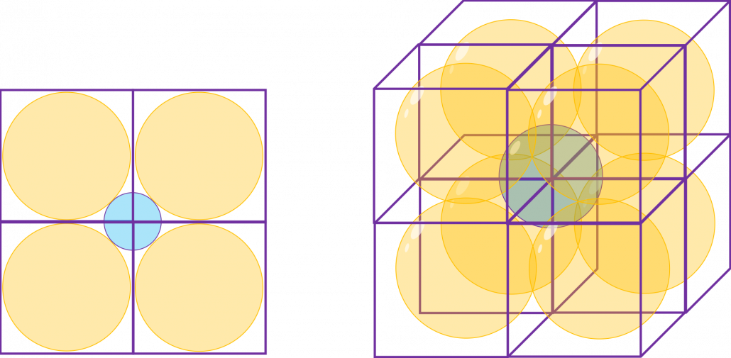
 , and the diameter of the blue sphere is
  .
. . If that is true, there is one strange point:
  can soon surpass 2: that means in the chart above the blue sphere will stick out of the stacked cubes. That sounds like a paradox, but with one hypothesis, the phenomenon makes sense: cubes become more spiky as the degree of dimension grows. This hypothesis is a natural deduction because diagonal lines of hyper cubes get longer, and the the center of each surface of hypercubes still touches the unit D-ball with diameter 1, inscribing inscribing inside each unit hypercube.
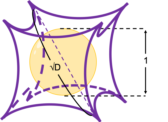
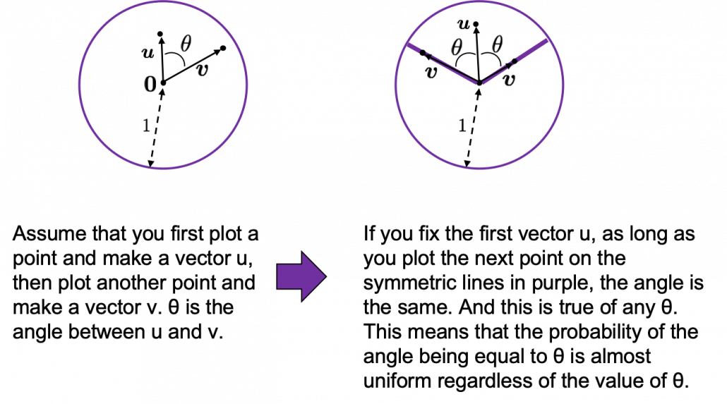
 . Let’s see the general meaning of angle between two vectors in any dimensional spaces. Assume that the angle between two vectors
  , then
  is calculated as
  . In 1, 2, or 3 dimensional space, you can actually see the angle, but again you can define higher dimensional angle, which you cannot visualize anymore. And angles are sometimes used as similarity of two vectors.
 is the inner product of
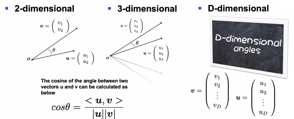
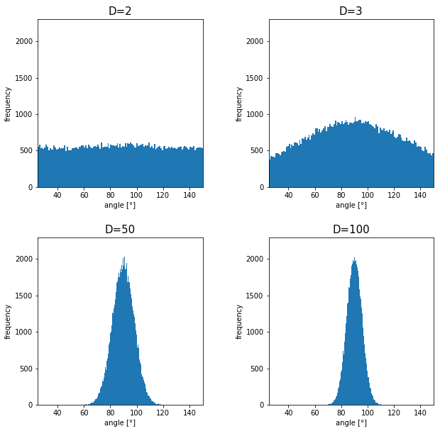
 How about in 3-dimensional space? In fact the distribution of
  is the most likely to be generated. As I explain in the figure below, if you compare the area of cross section of a hemisphere and the area of a cone whose vertex is the center point of the sphere, you can see why.
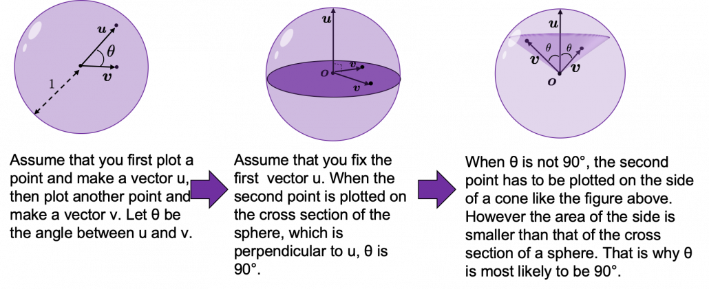
 surface of general spheres with radius
  First, in 2 two dimensional space, spheres are circles. The area of the brown part of the circle below is
  . In order calculate the are of
  thick surface of the circle, you have only to subtract the area of
  . When
  , the area of outer most surface is
  , and its proportion to the area of the whole circle is
  .
.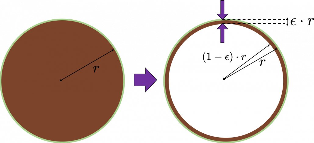
 , so the proportion of the
  . Compared to the case in 2 dimensional space, the proportion is a little bigger.
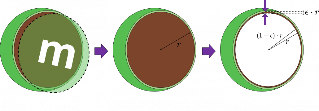

 is called gamma function, but in this article it is not so important. The most important point now is, if you discuss any D-ball, their volume only depends on their radius
  . When
  , and when
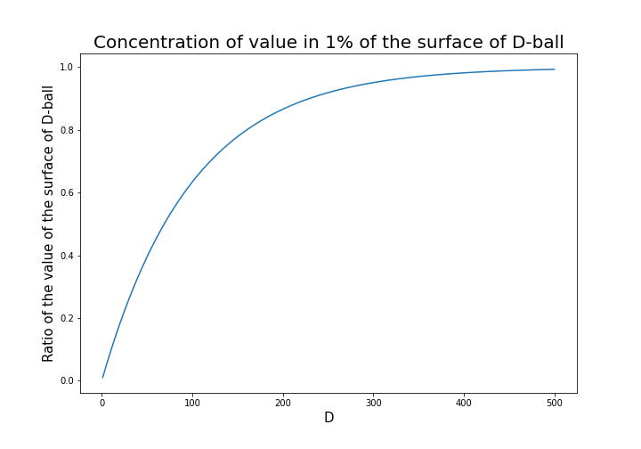
 radius of the center is almost zero. But if you reach the outermost