Automatic Financial Trading Agent for Low-risk Portfolio Management using Deep Reinforcement Learning
This article focuses on autonomous trading agent to solve the capital market portfolio management problem. Researchers aim to achieve higher portfolio return while preferring lower-risk actions. It uses deep reinforcement learning Deep Q-Network (DQN) to train the agent. The main contribution of their work is the proposed target policy.
Introduction
Author emphasizes the importance of low-risk actions for two reasons: 1) the weak positive correlation between risk and profit suggests high returns can be obtained with low-risk actions, and 2) customer satisfaction decreases with increases in investment risk, which is undesirable. Author challenges the limitation of Supervised Learning algorithm since it requires domain knowledge. Thus, they propose Reinforcement Learning to be more suitable, because it only requires state, action and reward specifications.
The study verifies the method through the back-test in the cryptocurrency market because it is extremely volatile and offers enormous and diverse data. Agents then learn with shorter periods and are tested for the same period to verify the robustness of the method.
2 Proposed Method
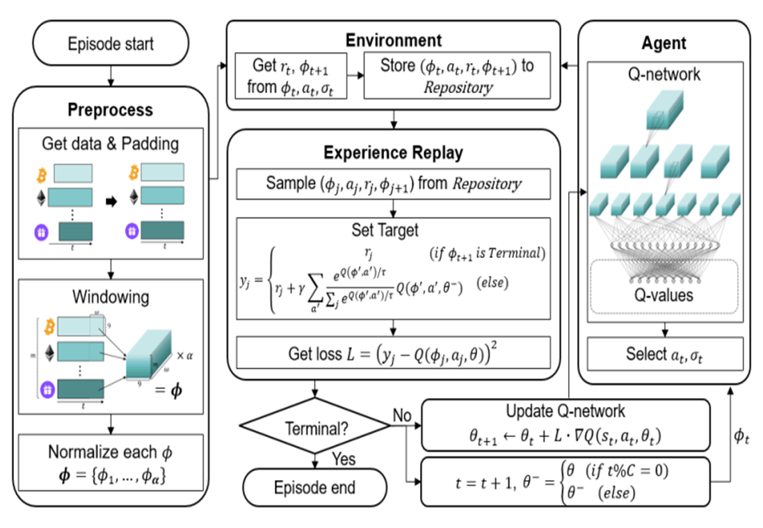
The overall structure of the proposed method is shown below.
2.1 Problem Definition
The portfolio consists of m assets and one base currency.
The price vector p stores the price p of all assets:
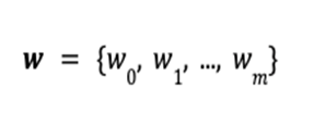
The portfolio vector w stores the amount of each asset:
At time ![]() , the total value
, the total value ![]() of the portfolio is defined as the inner product of the price vector
of the portfolio is defined as the inner product of the price vector ![]() and the portfolio vector
and the portfolio vector ![]() .
.
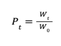
Finally, the goal is to maximize the profit ![]() at the terminal time step
at the terminal time step ![]() .
.
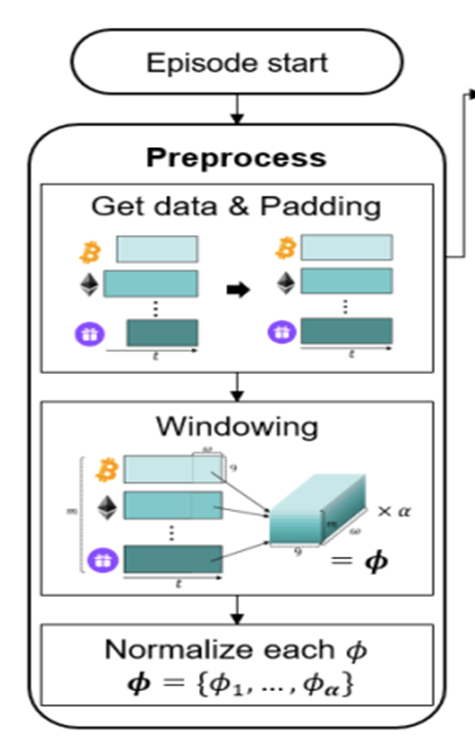
2.2 Asset Data Preprocessing
1) Asset Selection
Data is drawn from the Binance Exchange API, where top m traded coins are selected as assets.
2) Data Collection
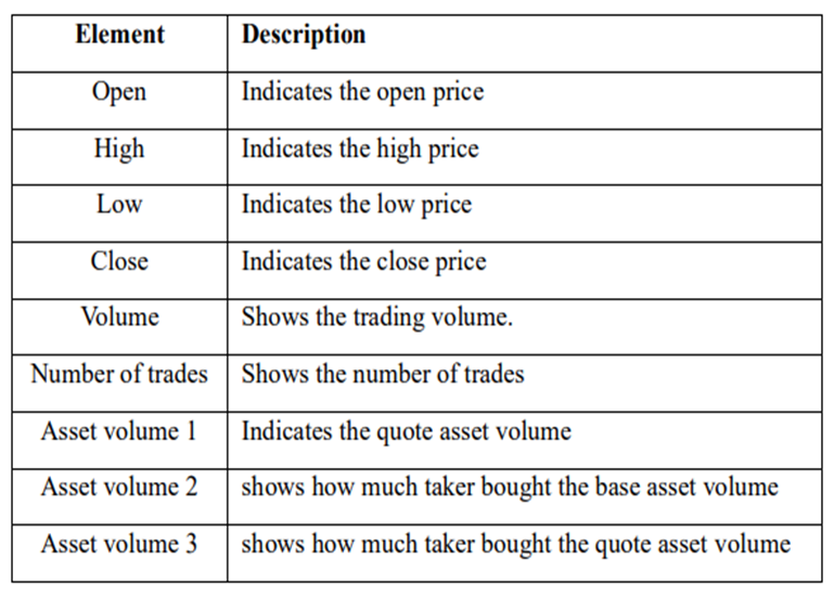
Each coin has 9 properties, shown in Table.1, so each trade history matrix has size (α * 9), where α is the size of the target period converted into minutes.
3) Zero-Padding
Pad all other coins to match the matrix size of the longest coin. (Coins have different listing days)
Comment: Author pointed out that zero-padding may be lacking, but empirical results still confirm their method covering the missing data well.
4) Stack Matrices
Stack m matrices of size (α * 9) to form a block of size (m* α * 9). Then, use sliding window method with widow size w to create (α – w + 1) number of sequential blocks with size (w * m * 9).
5) Normalization
Normalize blocks with min-max normalization method. They are called history block 𝜙 and used as input (ie. state) for the agent.
3. Deep Q-Network
The proposed RL-based trading system follows the DQN structure.
Deep Q-Network has 2 networks, Q- and Target network, and a component called experience replay. The Q-network is the agent that is trained to produce the optimal state-action value (aka. q-value).
Comment: Q-value is calculated by the Bellman equation, which, in short, consists of the immediate reward from next action, and the discounted value of the next state by following the policy for all subsequent steps.
Here,
Agent: Portfolio manager
Action a: Trading strategy according to the current state
State 𝜙 : State of the capital market environment
Environment: Has all trade histories for assets, return reward r and provide next state 𝜙’ to agent again
DQN workflow:
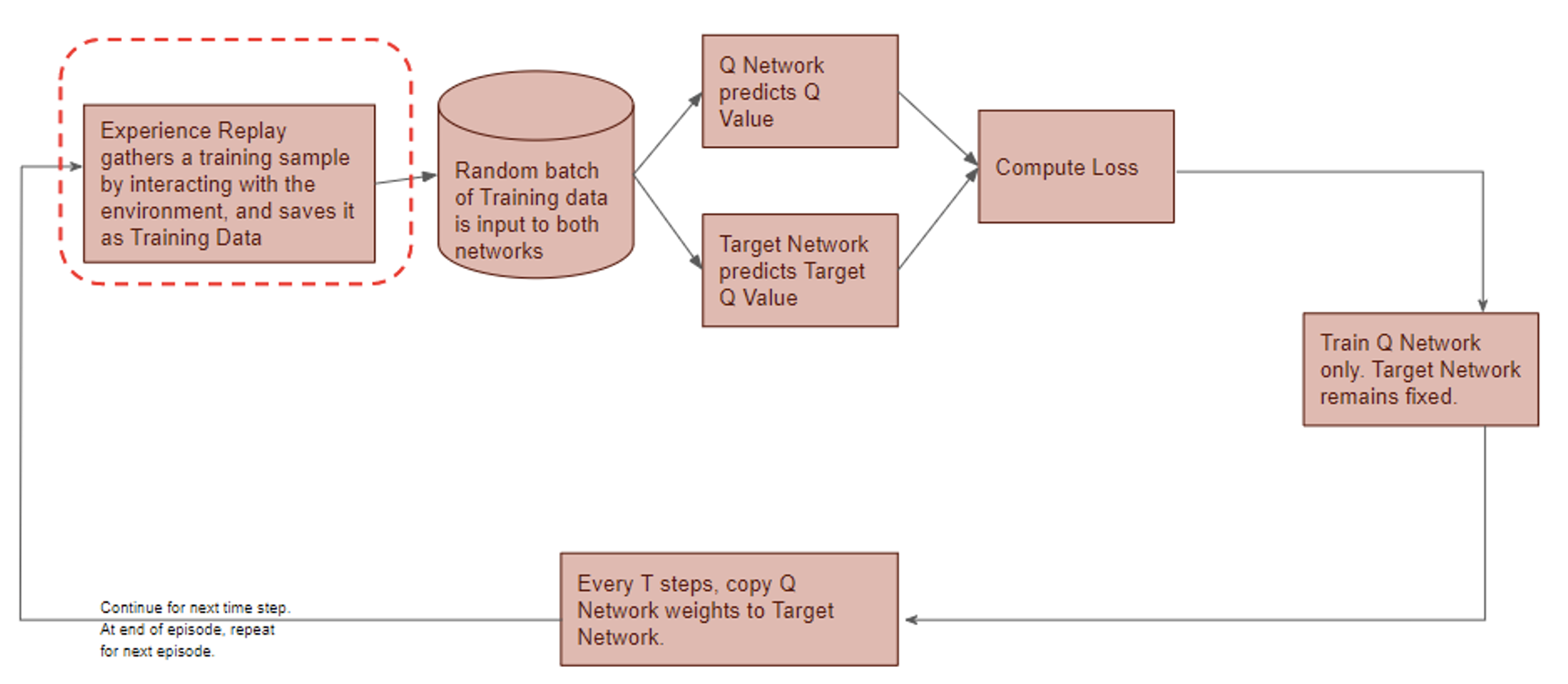
DQN gets trained in multiple time steps of multiple episodes. Let’s look at the workflow of one episode.
1) Experience replay selects an action according to the behavior policy, executes in the environment, returns the reward and next state. This experience set (![]() ) is stored in the repository as a sample of training data.
) is stored in the repository as a sample of training data.
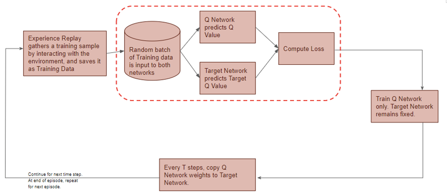
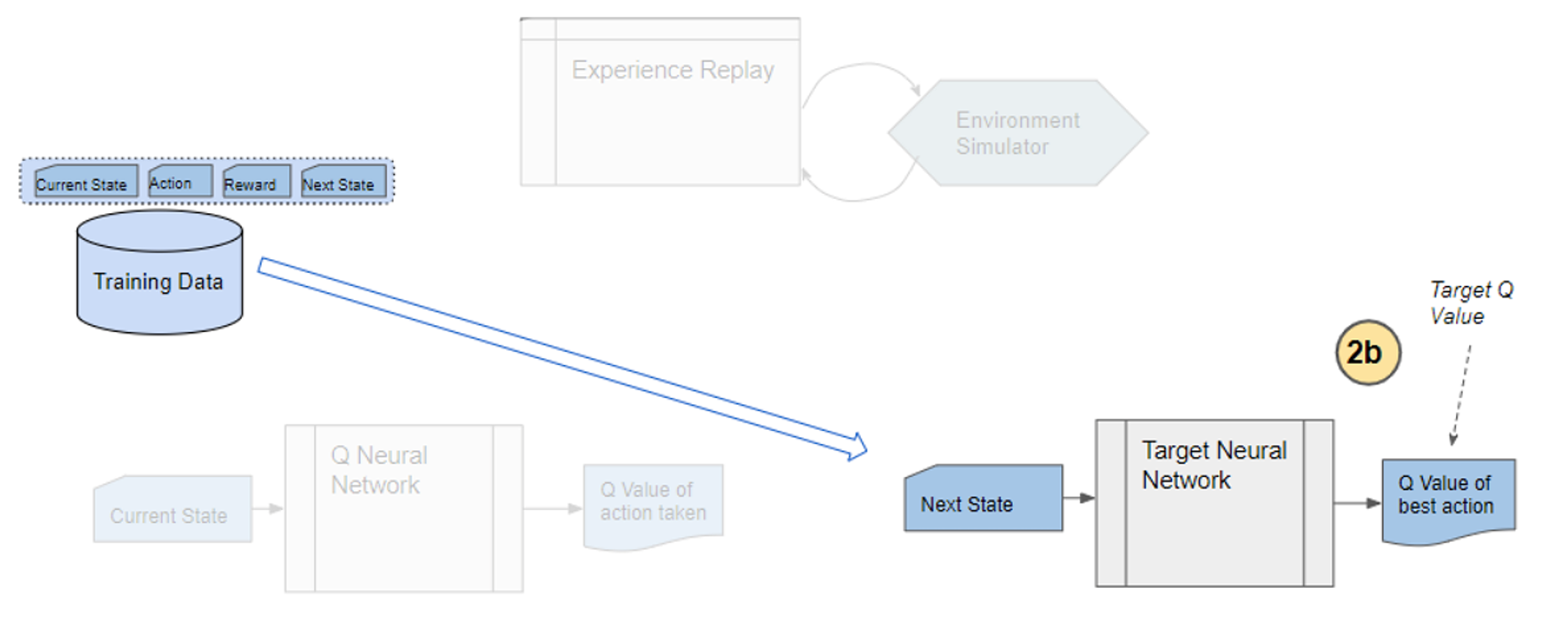
2) From the repository of prior observations, take a random batch of samples as the input to both Q- and Target network. The Q-network takes the current state and action from each data sample and predicts the q-value for that particular action. This is the ‘Predicted Q-Value’.Comment: Author uses 𝜀-greedy algorithm to calculate q-value and select action. To simplify, 𝜀-greedy policy takes the optimal action if a randomly generated number is greater than 𝜀, which represents a tradeoff between exploration and exploitation.
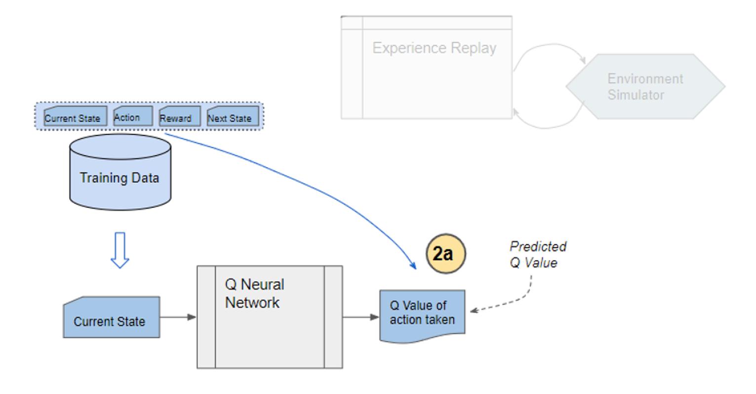 The Target network takes the next state from each data sample and predicts the best q-value out of all actions that can be taken from that state. This is the ‘Target Q-Value’.
Comment: Author proposes a different target policy to calculate the target q-value.
3) The Predicted q-value, Target q-value, and the observed reward from the data sample is used to compute the Loss to train the Q-network.
Comment: Target Network is not trained. It is held constant to serve as a stable target for learning and will be updated with a frequency different from the Q-network.
4) Copy Q-network weights to Target network after n time steps and continue to next time step until this episode is finished.
4.0 Main Contribution of the Research
4.1 Action and Reward
Agent determines not only action a but ratio , at which the action is applied.
- Action:
Hold, buy and sell. Buy and sell are defined discretely for each asset. Hold holds all assets. Therefore, there are (2m + 1) actions in the action set A.

Agent obtains q-value of each action through q-network and selects action by using 𝜀-greedy algorithm as behavior policy. - Ratio:
 is defined as the softmax value for the q-value of each action (ie. i-th asset at
  , then i-th asset is bought using 50% of base currency).

- Reward:
Reward depends on the portfolio value before and after the trading strategy. It is clipped to [-1,1] to avoid overfitting.
4.2 Proposed Target Policy
Author sets the target based on the expected SARSA algorithm with some modification.
Comment: Author claims that greedy policy ignores the risks that may arise from exploring other outcomes other than the optimal one, which is fatal for domains where safe actions are preferred (ie. capital market).
The proposed policy uses softmax algorithm adjusted with greediness according to the temperature term 𝜏. However, softmax value is very sensitive to the differences in optimal q-value of states. To stabilize learning, and thus to get similar greediness in all states, author redefine 𝜏 as the mean of absolute values for all q-values in each state multiplied by a hyperparameter 𝜏’.
4.3 Q-Network Structure
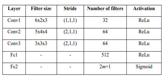
This study uses Convolutional Neural Network (CNN) to construct the networks. Detailed structure of the networks is shown in Table 2.
Comment: CNN is a deep neural network method that hierarchically extracts local features through a weighted filter. More details see: https://towardsdatascience.com/stock-market-action-prediction-with-convnet-8689238feae3.
5 Experiment and Hyperparameter Tuning
5.1 Experiment Setting
Data is collected from August 2017 to March 2018 when the price fluctuates extensively.
Three evaluation metrics are used to compare the performance of the trading agent.
- Profit
 introduced in 2.1.
 - Sharpe Ratio: A measure of return, taking risk into account.

Comment: is the standard deviation of the expected return and
  is the return of a risk-free asset, which is set to 0 here.
 - Maximum Drawdown: Maximum loss from a peak to a through, taking downside risk into account.

5.2 Hyperparameter Optimization
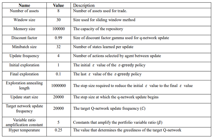
The proposed method has a number of hyperparameters: window size mentioned in 2.2, 𝜏’ in the target policy, and hyperparameters used in DQN structure. Author believes the former two are key determinants for the study and performs GridSearch to set w = 30, 𝜏’ = 0.25. The other hyperparameters are determined using heuristic search. Specifications of all hyperparameters are summarized in the last page.
Comment: Heuristic is a type of search that looks for a good solution, not necessarily a perfect one, out of the available options.
5.3 Performance Evaluation
Benchmark algorithms:
UBAH (Uniform buy and hold): Invest in all assets and hold until the end.
UCRP (Uniform Constant Rebalanced Portfolio): Rebalance portfolio uniformly for every trading period.
Methods from other studies: hyperparameters as suggested in the studies
EG (Exponential Gradient)
PAMR (Passive Aggressive Mean Reversion Strategy)
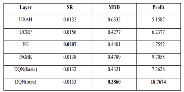
Comment: DQN basic uses greedy policy as the target policy.
The proposed DQN method exhibits the best overall results out of the 6 methods. When the agent is trained with shorter periods, although MDD increases significantly, it still performs better than benchmarks and proves its robustness.
6 Conclusion
The proposed method performs well compared to other methods, but there is a main drawback. The encoding method lacked a theoretical basis to successfully encode the information in the capital market, and this opaqueness is a rooted problem for deep learning. Second, the study focuses on its target policy, while there remains room for improvement with its neural network structure.
References
- Shin, S. Bu and S. Cho, “Automatic Financial Trading Agent for Low-risk Portfolio Management using Deep Reinforcement Learning”, https://arxiv.org/pdf/1909.03278.pdf
- Li, P. Zhao, S. C. Hoi, and V. Gopalkrishnan, “PAMR: passive aggressive mean reversion strategy for portfolio selection,” Machine learning, vol. 87, pp. 221-258, 2012.
- P. Helmbold, R. E. Schapire, Y. Singer, and M. K. Warmuth, “On‐line portfolio selection using multiplicative updates,” Mathematical Finance, vol. 8, pp. 325-347, 1998.
http://www.kasimte.com/2020/02/14/how-does-temperature-affect-softmax-in-machine-learning.html





 DATANOMIQ


Leave a Reply
Want to join the discussion?Feel free to contribute!