Stop saying “trial and errors” for now: seeing reinforcement learning through some spectrums
*This is the fourth article of the series My elaborate study notes on reinforcement learning.
*In this article series “the book by Barto and Sutton” means “Reinforcement Learning: An Introduction second edition.” This book is said to be almost mandatory for those who seriously learn Reinforcement Learning (RL). And “the whale book” means a Japanese textbook named 「強化学習 (機械学習プロフェッショナルシリーズ)」(“Reinforcement Learning (Machine Learning Processional Series)”), by Morimura Tetsuro. I would say the former is for those who want to mainly learn how to use RL, and the latter is for more theoretical understanding. I am trying to make something between them in my series.
1, Finally to reinforcement learning
Some of you might have got away with explaining reinforcement learning (RL) only by saying an obscure thing like “RL enables computers to learn through trial and errors.” But if you have patiently read my articles so far, you might have come to say “RL is a family of algorithms which simulate procedures similar to dynamic programming (DP).” Even though my article series has not covered anything concrete and unique to RL yet, I think my series has already laid a hopefully effective foundation of discussions on RL. And in the first article, I already explained that “trial and errors” are only agents’ actions for collecting data from the environment. Such “trial and errors” lead to “experiences” of computers. And in this article we can finally start discussing how computers “experience” things in more practical and theoretical ways.
*The expression “to learn” is also frequently used in contexts of other machine learning algorithms. Thus in order to clearly separate the ideas, let me use the expression “to experience” when it comes to explaining RL. At any rate, what computers are doing is updating parameters, and in RL also updating values and policies. But some terms related to RL also use the word “experience,” for example experience replay, so “to experience” might be a preferred phrase in RL fields.
I think changing discussions on DP into those on RL is like making graphs more “open” rather than “closed.” In the second article, I explained DP problems, where the models of environments are completely known, as repeatedly updating graphs like neural networks. As I have been repeatedly saying RL, or at least model-free RL, is an approximated application of DP in the environments without a complete model. That means, connections of nodes of the graph, that is relations of actions and states, are something agents have to estimate directly or indirectly. I think that can be seen as untying connections of the graphs which I displayed when I explained DP. By doing so, I propose to see RL or more exactly model-free RL like the graph of the right side of the figure below.

*For the time being, I would prefer to use the term model-free RL rather than just RL. That is not only because this article is about model-free RL but also because I want to avoid saying inaccurate things about wider range of RL algorithms I would have to study more precisely and explain.
Some people might say these are tree structures, and that might be technically correct. But in my sense, this is more of “willows.” The cover of the second edition of the books by Barto and Sutton also looks like willows. The cover design comes from a paper on RL named “Learning to Drive a Bicycle using Reinforcement Learning and Shaping.” The paper is about learning to ride a bike in a simulator with RL. The geometric patterns are not models of human brain nerves, but trajectories of an agent learning to balance a bike. However interestingly, the trajectories of the bike, which are inscribed on a road, partly diverge but converge in a certain way as a whole, like the RL graph I propose. That is why I chose some pictures of 「花札 (hanafuda)」as the main picture of this series. Hanafuda is a Japanese gamble card game with monthly seasonal flower pictures. And the cards of June have pictures of willows.

Source: Learning to Drive a Bicycle using Reinforcement Learning and Shaping, Randløv, (1998) Richard S. Sutton, Andrew G. Barto, “Reinforcement Learning: An Introduction,” MIT Press, (2018)
2, Untying DP graphs: planning or learning
Even though I have just loudly declared that my RL graphs are more of “willow” structures in my aesthetic sense, I must admit they should basically be discussed as popular tree structures. That is because, when you start discussing practical RL algorithms you need to see relations of states and actions as tree structures extending. If you already more or less familiar with tree structures or searching algorithms on tree graphs, learning RL with tree structures should be more or less straightforward to you. Another reason for using tree structures with nodes of states and actions is that the book by Barto and Sutton use buck up diagrams of Bellman equations which are tree graphs. But I personally think the graphs should be used more effectively, so I am trying to expand its uses to DP and RL algorithms in general. In order to avoid confusions about current discussions on RL in my article series, I would like to give an overall review on how to look at my graphs.
The graphs in the figure below are going to be used in my articles, at least when I talk about model-free RL. I made them based on the backup diagram of Bellman equation introduced in the book by Barto and Sutton. I would like you to first remember that in RL we are basically discussing Markov decision process (MDP) environment, where the next action and the resulting next states depends only on the current state. Such models are composed of white nodes representing each state  in an state space
  , and black nodes representing each action
  , which is a member of an action space
  . Any behaviors of agents are represented as going back and forth between black and white nodes of the model, and that is why connections in the MDP model are bidirectional. In my articles let me call such model of environments “a closed model.” RL or general planning problems are matters of optimizing policies in such models of environments. Optimizing the policies are roughly classified into two types, planning/searching or RL, and the main difference between them is whether connections of graphs of models are known or not. Planning or searching is conducted without actually moving in the environment. DP are family of planning algorithms which are known to converge, and so far in my articles we have seen that DP are enabled by repeatedly applying Bellman operators. But instead of considering and updating all the possible transitions in the model like DP, planning can be conducted more sparsely. Such sparse planning are often called searching, and many of them use tree structures. If you have learned any general decision making problems with tree graphs, you might be already familiar with some searching techniques like alpha-beta pruning.

*In explanations on DP in my articles, directions of connections of model graphs are confusing, so I precisely explained how to look at them in the second section in the last article.
On the other hand, RL algorithms are matters of learning the linkages of models of environments by actually moving in them. For example, when the agent in the figure below move on a grid map like the purple arrows, the movement is represented like in the closed model in the middle. However as the agent does not have the complete closed model, the agent has to move around in the environment like the tree structure at the right side to learn values of each node.
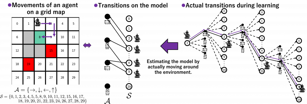
The point is, whether models of environments are known or unknown, or whether agents actually move in the environment or not, movements of agents are basically represented as going back and forth between white nodes and black nodes in closed models. And such closed models are entangled in searching or RL. They are similar operations, but they are essentially different in that searching agents do not actually move in searching but in RL they actually move. In order to distinguish searching and learning, in my articles, trees for searching are extended vertically, trees for learning horizontally.
*DP and searching are both planning, but DP consider all the connections of actions and states by repeatedly applying Bellman operators. Thus I would not count DP as “untying” of closed models.
3, Some spectrums in RL algorithms
Starting studying actual RL algorithms also means encountering various algorithms one after another. Some of you might have already been overwhelmed by new terms coming up one after another in study materials on RL. That is because, as I explained in the first article, RL is more about how to train models of values or policies. Thus it is natural that compared to general machine learning, which more or less share the same training frameworks, RL has a variety of training procedures. Rather than independently studying each RL algorithm, I think it is more effective to see connections of each algorithm, which is linked by adjusting degrees of some important elements in RL. In fact I have already introduced those elements as some pairs of key words of RL in the first article. But it would be all the more effective to review them, especially after learning DP algorithms as representative planning methods. If you study RL that way, you would come to see trial and errors or RL as a crucial but just one aspect of RL.
I think if you care less about the trial-and-error aspect of RL that allows you to study RL more effectively in the beginning. And for the time being, you should stop viewing RL in the popular way as presented above. Not that I am encouraging you to ignore the trial and error part, namely relations of actions, rewards, and states. My point is that it is more of inside the agent that should be emphasized. Planning, including DP is conducted inside the agent, and trial and errors are collection of data from the environment for the sake of the planning. That is why in many study materials on RL, DP is first introduced. And if you see differences of RL algorithms as adjusting of some pairs of elements of planning problems, it would be less likely that you would get lost in curriculums on RL. The pairs are like some spectrums. Not that you always have to choose either of each pair, but rather ideal solutions are often in the middle of the two ends of the spectrums depending on tasks. Let’s take a look at the types of those spectrums one by one.
(1) Value-policy or actor-critic spectrum
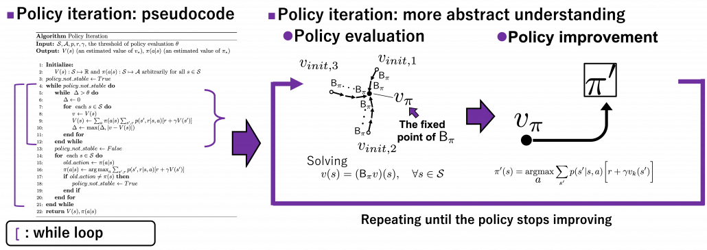
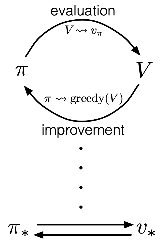
The crucial type of spectrum you should be already familiar with is the value-policy one. I think this spectrum can be adjusted in various ways. For example, over the last two articles we have seen how values and policies reach the optimal functions in DP using policy iteration or value iteration. Policy iteration alternates between updating values and policies until convergence to the optimal policy, whereas value iteration keeps updating only values until reaching the optimal value, to get the optimal policy at the end. And similar discussions can be seen also in the upcoming RL algorithms. The book by Barto and Sutton sees such operations in general as generalized policy iteration (GPI).
Source: Richard S. Sutton, Andrew G. Barto, “Reinforcement Learning: An Introduction,” MIT Press, (2018)
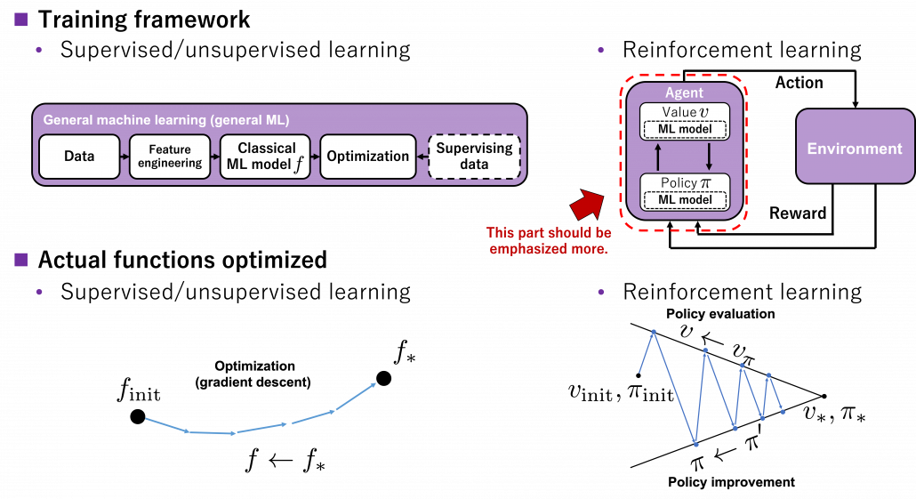
You should pay attention to the idea of GPI because this is what makes RL different form other general machine learning. In many cases RL is explained as a field of machine learning which is like trial and errors, but I personally think that GPI, interactive optimization between values and policies, should be more emphasized. As I said in the first article, RL optimizes decision making rules, that is policies  , in MDPs. Other general machine learning algorithms have more direct supervision by loss functions and models are optimized so that loss functions are minimized. In the case of the figure below, an ML model
  is optimized to
  by optimization such as gradient descent. But on the other hand in RL policies
  do not have direct loss functions. Then RL uses values
  , which are functions of how good it is to be in states . As one part of GPI, the value function
  for the current policy is calculated, and this is called estimation in the book by Barto and Sutton. And based on the estimated value function, the policy is improved as
  , which is called policy improvement, and overall processes of estimation and policy improvement are called control in the book. And and are updated alternately this way until converging to the optimal values
  or policies
  . This interactive updates of values and policies are done inside the agent, in the dotted frame in red below. I personally think this part should be more emphasized than trial-and-error-like behaviors of agents. Once you see trial and errors of RL as crucial but just one aspect of GPI and focus more inside agents, you would see why so many study materials start explaining RL with DP.
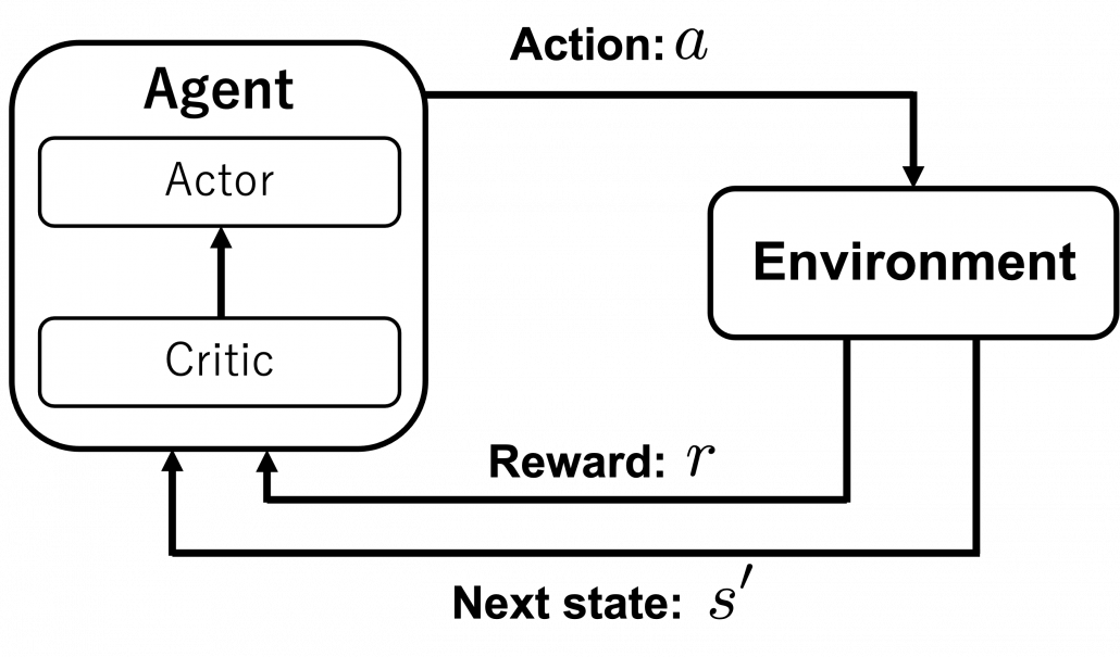
You can explicitly model such interactions of values and policies by modeling each of them with different functions, and in this case such frameworks of RL in general are called actor-critic methods. I am gong to explain actor-critic methods in an upcoming article. Thus the value-policy spectrum also can be seen as a actor-critic spectrum. Differences between the pairs of value-policy or actor-critic spectrums are something you would little by little understand. For now I would say GPI is the most general and important idea behind RL. But practical RL algorithms are implemented as actor-critic methods. Critic parts gives some signals to actor parts, and critic parts get its consequence by actor parts taking actions in environments. Not that actors directly give feedback to critics.
*I think one of confusions in studying RL come from introducing Q-learning or SARSA at the first algorithms or a control in RL. As I have said earlier, interactive relations between values and policies or actors and critics, that is GPI, should be emphasized. And I think that is why DP is first introduced in many books. But in Q-learning or SARSA, an actor and a critic parts are combined as one module. But explicitly separating the actor and critic parts would be just too difficult at the beginning. And modeling an actor and a critic with separate modules would lead to difficulties in optimizing them together.
(2) Exploration-exploitation or on-off policy spectrum
I think the most straightforward spectrum is the exploitation-exploration spectrum. You can adjust how likely agents take random actions to collect data. Occasionally it is ideal for agents to have some degree of randomness in taking actions to explore unknown states of environments. One of the simplest algorithms to formulate randomness of actions is ε-greedy method, which I explained in the first article. In this method in short agents take a random action with a probability of ε. Instead of arbitrarily setting a hyperparameter  , randomness of actions can be also learned by modeling policies with certain functions. This randomness of functions can be also modeled in actor-critic frameworks. That means, depending on a choice of an actor, such actor can learn randomness of actions, that is explorations.
The two types of spectrums I have introduced so far lead to another type of spectrum. It is an on-off policy spectrum. Even though I explained types of policies in the last article using examples of home-lab-Starbucks diagrams, there is another way to classify policies: there are target policies and behavior policies. The former are the very policies whose optimization we have been discussing. The latter are policies for taking actions and collecting data. When agents use target policies also as behavior policies, they are on-policy algorithms. If agents use different policies for taking actions during optimization of target policies, they are off-policy methods.
Policy iteration and value iteration of DP can be also classified into on-policy or off-policy in a sense. In policy iteration values are updated using an up-to-date estimated policy, and the policy becomes optimal when it converges. Thus behavior and target policies are the same in this case. On the other hand in value iteration, values are updated with Bellman optimality operator, which updates values in a greedy way. Using greedy method means the policy is not used for considering which action to take. Thus target and behavior policies are different. As you will see soon, concrete model-free RL algorithms like SARSA or Q-learning also have the same structure: the former is on-policy and the latter is off-policy. The difference of on-policy or off-policy would be more straightforward if we model behavior policies and target policies with different functions. An advantage of off-policy RL is you can model randomness of exploration of agents with extra functions. On the other hand, a disadvantage is that it would be harder to train different models at the same time. That might be a kind of tradeoff similar to an actor-critic method.
Even though this exploration-exploitation aspect of RL is relatively easy to understand, at the same time that can lead to much more complicated discussions on RL, which I would not be able to cover in this article series. I recommended you to stop seeing RL as trial and errors for the time being, but in the end trial and errors would prove to be crucial because data needed for GPI are collected mainly via trial and errors. Even if you implement some simple RL algorithms, you would soon realize it is hard to deal with unvisited states. Enough explorations need to be modeled by a behavior policy or some sophisticated heuristic techniques. I am planning to explain convergence of several RL algorithms, and they are guaranteed by sufficiently exploring all the states. However, thorough explorations of all the states lead to massive computational costs. But lack of exploration would let RL agents myopically overestimate current policies, never finding policies which pay off in the long run. That might be close to discussions on how to efficiently find a global minimum of a loss function, avoiding local minimums.
(3) TD-MonteCarlo spectrum
A variety of spectrums so far are enabled by modeling proper functions on demand. But in AI problems such functions are something which have to be automatically trained with some supervision. Instead of giving supervision explicitly with annotated data like in supervised learning of general machine learning, RL agents train models with “experiences.” As I am going to explain in the next part of this article, “experiences” in RL contexts mean making some estimations of values and adjusting such estimations based on actual rewards they get. And the timings of such feedback lead to another spectrum, which I call a TD-MonteCarlo spectrum. When the feedback happens every time an agent takes an action, it is TD method, on the other hand when that happens only at the end of an episode, that is Monte Carlo method. But it is easy to imagine that ideal solutions are usually at the middle of them. I am going to dig this topic soon in the next article. And n-step methods or TD(λ), which bridge the TD and Monte Carlo, are going to be covered in one of upcoming articles.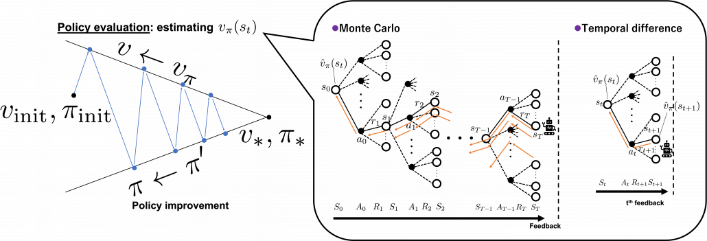
(4) Model free-based spectrum
The next spectrum might be relatively hard to understand, and to be honest I am still not completely sure about this topic. Please bear that in your mind. In the last section, I said RL is a kind of untying DP graphs and make them open because in RL, models of environments are unknown. However to be exact, that was mainly about model-free RL, which this article is going to cover for the time being. And I would say the graphs I showed in the last section were just two extremes of this model based-free spectrum. Some model-based RL methods exist in the middle of those two ends. In short RL agents can retain models of environments and do some plannings even when they do trial and errors. The figure below briefly compares planning, model-based RL, and model-free RL in the spectrum.
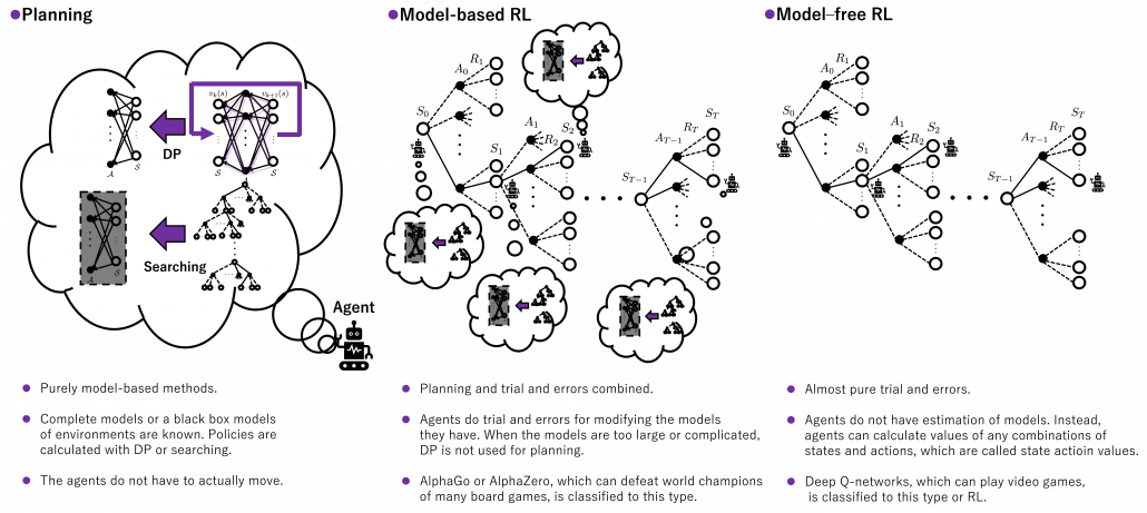
Let’s take a rough example of humans solving a huge maze. DP, which I have covered is like having a perfect map of the maze and making plans of how to move inside in advance. On the other hand, model-free reinforcement learning is like soon actually entering the maze without any plans. In model-free reinforcement learning, you only know how big the maze is, and you have a great memory for remembering in which directions to move, in all the places. However, as the model of how paths are connected is unknown, and you naively try to remember all the actions in all the places, it generally takes a longer time to solve the maze. As you could easily imagine, having some heuristic ideas about the model of the maze and taking some notes and making plans about courses would be the most efficient and the most peaceful. And such models in your head can be updated by actually moving in the maze.
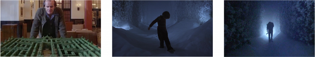
*I believe that you would not say the pictures above are spoilers.
I need to more clearly talk about what a model is in RL or general planning problems. The book by Barto and Sutton simply defines a model this way: “By a model of the environment we mean anything that an agent can use to predict how the environment will respond to its actions. ” The book also says such models can be also classified to distribution models and sample models. The difference between them is the former describes an environment as combinations of known models, but the latter is like a black box model of an environment. An intuitive example is, as introduced in the book by Barto and Sutton, throwing dozens of dices can be seen in the both types. If you just throw the dices, sometimes chancing numbers of dices, and record the sum of the numbers on the dices s every time, that is equal to getting the sum from a black box. But a probabilistic distribution of such sums can be actually calculated as a multinomial distribution. Just as well, you can see a probability of transitions in an RL environment as a black box, but the probability can be also modeled. Some readers might have realized that distribution or sample models can be almost the same in the end, with sufficient data. In many cases of machine learning or statistics algorithms, complicated distributions have to be approximated with samples. Or rather how to approximate them is more of interest. In the case of dozens of dices, you can analytically calculate its distribution model as a multinomial distribution. But if you throw the dices numerous times, you would get precise approximated distributions.
When we discuss model-based RL, we need to consider not only DP but also other planning algorithms. DP is a family of planning algorithms which are known to converge, and many of RL algorithms share a lot with DP at theoretical levels. But in fact DP has one shortcoming even if the MDP model of an environment is known: DP needs to consider and update all the states. When models of environments are too complicated and large, applying DP is not a good idea. Also in many of such cases, you could not even get such a huge model of the environment. You would rather get only a black box model of the environment. Such a black box model only gets a pair of current state and action  , and gives out the next state
  and corresponding reward
  , that is the black box is a sample model. In this case other planning methods with some searching algorithms are used, for example Monte Carlo tree search. Such search algorithms are designed to more efficiently and sparsely search states and actions of interest. Many of searching algorithms used in RL make uses of tree structures. Model-based approaches can be roughly classified into three types below based on size or complication of models.
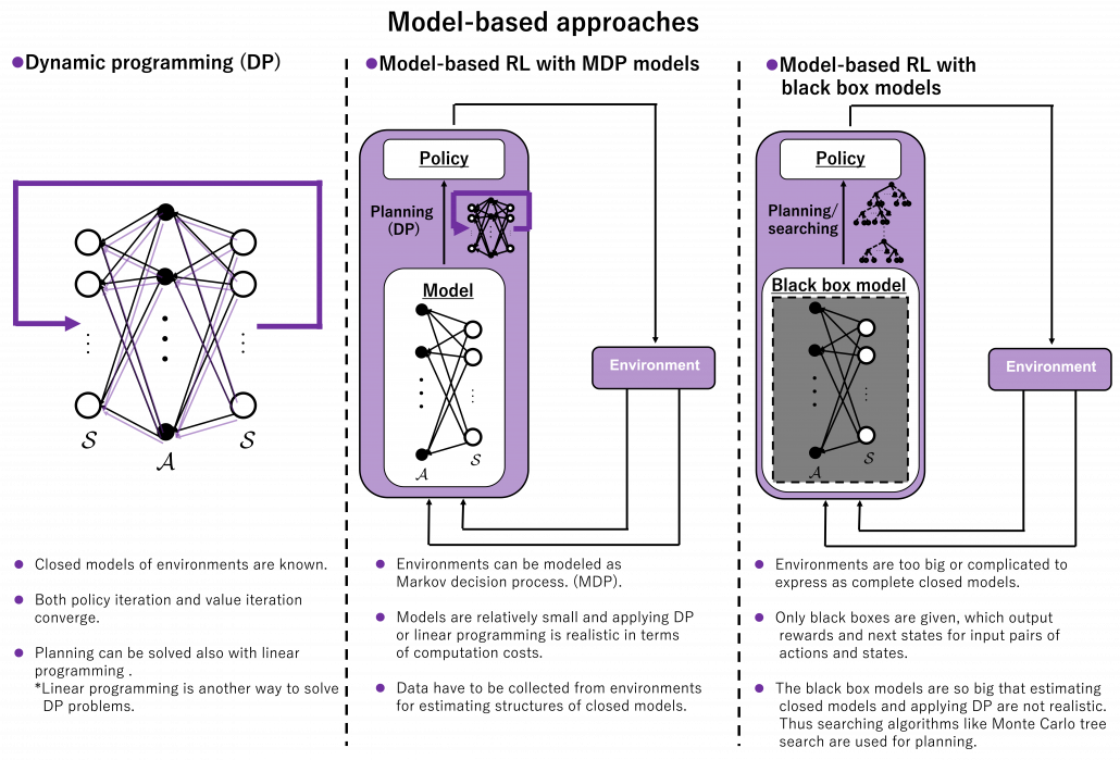
*As you could see, differences between sample models and distribution models can be very ambiguous. So are differences between model-free and model-based RL, I guess. As a matter of fact the whale book says the distributions of models approximated in model-free RL are the same as those in model-based ones. I cannot say anything exactly anymore, but I guess model-free RL is more of “memorizing” an environment, or combinations of states and actions in the environments. But memorizing environments can be computationally problematic in many cases, so assuming some distributions of models can help. That is my impression for now.
*Tree search algorithms alone shows very impressive performances, as long as you have massive computation resources. A heuristic tree search without reinforcement learning could defeat Garri Kasparow, a former chess champion, as long as enough computation resource is available. Searching algorithms were enough for “simplicity” of chess.
*I am not sure whether model-free RL algorithms are always simpler than model-based ones. For example Deep Q-Learning, a model-free method with some neural networks can learn to play Atari or Nintendo Entertainment System. Model-based deep RL is used in more complex task like AlphaGo or AlphaZero, which can defeat world champions of various board games. AlphaGo or AlphaZero models intuitions in phases of board games with convolutional neural networks (CNN), prediction of some phases ahead with search algorithms, and learning from past experiences with RL. I am not going to cover model-based RL in general in this series, but instead I would like to explain how RL enables computers to play video games after introducing some searching algorithms.
(5) Model expressivity spectrum
No matter how impressive or dreamy RL algorithms sound, their competence largely depend on model expressivity. In the first article, I emphasized “simplicity” of RL. DP or RL algorithms so far or in upcoming several articles consider incredibly simple cases like kids playbooks. And that beginning parts of most RL study materials cover only the left side of the figure below. In order to enable RL agents with more impressive tasks such as balancing cart-pole or playing video games, we need to raise the bar of expressivity spectrum, from the left to the right side of the figure below. You need to wait until a chapter or a section on “function approximation” in order to actually feel that your computer is doing trial and errors. And such chapters finally appear after reading half of both the book by Barto and Sutton and the whale book.
 *And this spectrum is also a spectrum of computation costs or convergence. The left type could be easily implemented like programming assignments of schools since it in short needs only Excel sheets, and you would soon get results. The middle type would be more challenging, but that would not b computationally too expensive. But when it comes to the type at the right side, that is not something which should be done on your local computer. At least you need a GPU. You should expect some hours or days even for training RL agents to play 8 bit video games. That is of course due to cost of training deep neural networks (DNN), especially CNN. But another factors is potential inefficiency of RL. I hope I could explain those weak points of RL and remedies for them.
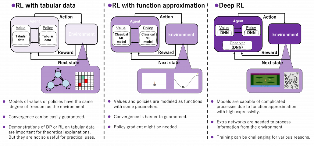
We need to model values and policies with certain functions. For the time being, in my articles values and policies are just modeled as tabular data, that is some NumPy arrays or Excel sheets. These are types of cases where environments and actions are relatively simple and discrete. Thus they can be modeled with some tabular data with the same degree of freedom. Assume a case where there are only 30 grids in an environment and only 4 types of actions in every grid. In such case, values are stored as arrays with 30 elements, and so are policies. But when environments are more complex or require continuous values of some parameters, values and policies have to be approximated with some models. When only relatively few parameters need to be estimated, simple machine learning models such as softmax functions can be used as such models. But compared to the cases with tabular data, convergence of training has to be discussed more carefully. And when you need to estimate continuous values, techniques like policy gradients have to be introduced. And we can dramatically enhance expressivity of models with deep neural netowrks (DNN), and such RL is called deep RL. Deep RL has showed great progress these days, and it is capable of impressive performances. Deep RL often needs observers to process inputs like video frames, and for example convolutional neural networks (CNN) can be used to make such observers. At any rate, no matter how much expressivity RL models have, they need to be supervised with some signals just as general machine learning often need labeled data. And “experiences” give such supervisions to RL agents.
(6) Adjusting sliders of spectrum
As you might have already noticed, these spectrums are not something you can adjust independently like faders on mixing board. They are more like some sliders for adjusting colors, brightness, or chroma on painting software. If you adjust one element, other parts are more or less influenced. And even though there are a variety of colors in the world, they continuously change by adjusting those elements of colors. Just as well, even if each RL algorithms look independent, many of them share more or less the same ideas, and only some parts are different in terms of their degrees. When you get lost in the course of studying RL, I would like you to decompose the current topic into these spectrums of RL elements I have explained.

I hope my explanations so far changed how you see RL. In the first article I already said RL is approximation of DP-like procedures with data collected by trial and errors, but from now on I would explain it also this way: RL is a family of algorithms which enable GPI by adjusting some spectrums.
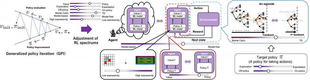
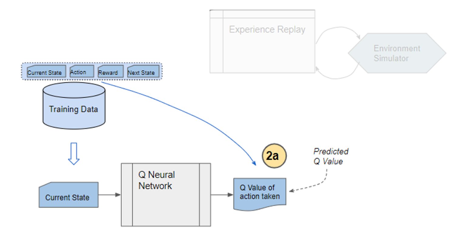
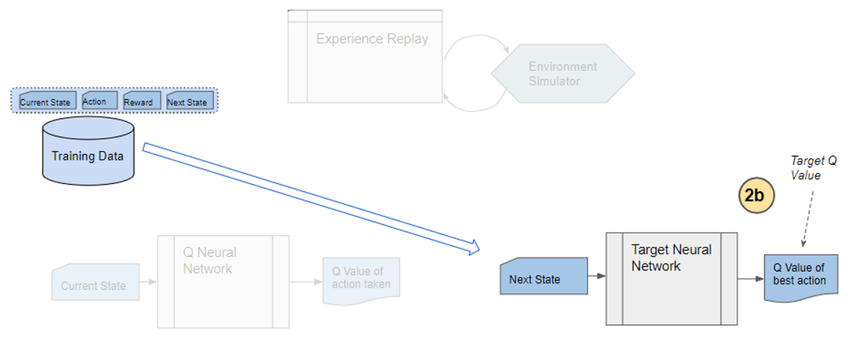
In the next some articles, I am going to mainly cover RL algorithms named SARSA and Q-learning. Both of them use tabular data, and they are model-free. And in values and policies, or actors and critics are together modeled as action-value functions, which I am going to explain later in this article. The only difference is SARSA is on-policy, and Q-learning is off-policy, just as I have already mentioned. And when it comes to how to train them, they both use Temporal Difference (TD), and this gives signals of “experience” to RL agents. Altering DP in to model-free RL is, in the figure above, adjusting the model-based-free and MonteCarlo-TD spectrums to the right end. And you also adjust the low-high-expressivity and value-policy spectrums to the left end. In terms of actor-critic spectrum, the actor and the critic parts are modeled as the same module. Seeing those algorithms this way would be much more effective than looking at their pseudocode independently.
* I make study materials on machine learning, sponsored by DATANOMIQ. I do my best to make my content as straightforward but as precise as possible. I include all of my reference sources. If you notice any mistakes in my materials, including grammatical errors, please let me know (email: yasuto.tamura@datanomiq.de). And if you have any advice for making my materials more understandable to learners, I would appreciate hearing it.

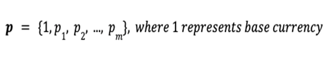
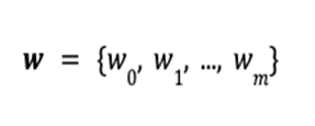
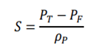
 , the total value
  of the portfolio is defined as the inner product of the price vector
  and the portfolio vector
  .
. at the terminal time step
  .
.
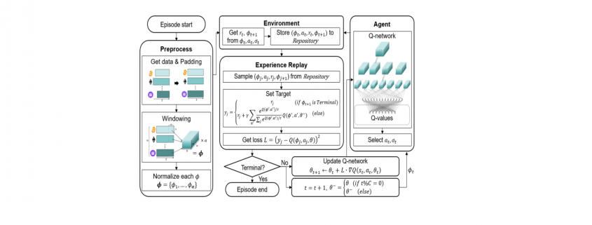
 ) is stored in the repository as a sample of training data.
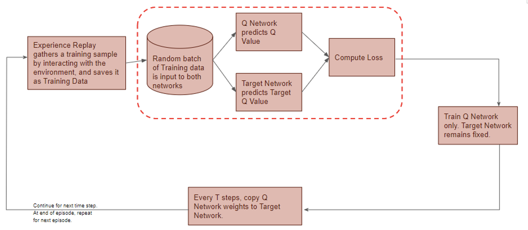
 is defined as the softmax value for the q-value of each action (ie. i-th asset at
  , then i-th asset is bought using 50% of base currency).
 is the return of a risk-free asset, which is set to 0 here.


 dependent variable.


 produces meaningful information of
  .
.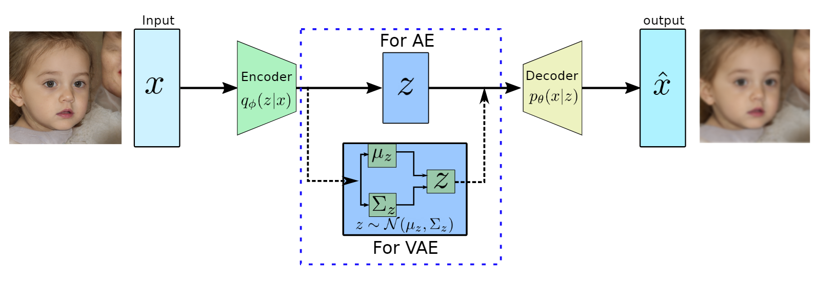
 usually has a much lower dimension than input
  and has the most dominant features of
 to approximate the conditional
  to generate images based on a sample from a true prior,
  are generally of Gaussian distribution.
 as it will be performing probabilistic generation of data. Therefore the encoder and decoder should be probabilistic.
 prior distribution, which is a Gaussian function, therefore, both of them are tractable. However, the integration won’t be tractable because of the high dimensionality of data.
 to approximate the conditional
  . Furthermore, the conditional
  , which is intractable. This additional encoder part will help to derive a lower bound on the data likelihood that will make the likelihood function tractable. In the following we will derive the lower bound of the likelihood function:
![\begin{equation*} \begin{flalign} \begin{aligned} log \: p_\theta (x) = & \mathbf{E}_{z\sim q_\phi(z|x)} \Bigg[log \: \frac{p_\theta (x|z) p_\theta (z)}{p_\theta (z|x)} \: \frac{q_\phi(z|x)}{q_\phi(z|x)}\Bigg] \\ = & \mathbf{E}_{z\sim q_\phi(z|x)} \Bigg[log \: p_\theta (x|z)\Bigg] - \mathbf{E}_{z\sim q_\phi(z|x)} \Bigg[log \: \frac{q_\phi (z|x)} {p_\theta (z)}\Bigg] + \mathbf{E}_{z\sim q_\phi(z|x)} \Bigg[log \: \frac{q_\phi (z|x)}{p_\theta (z|x)}\Bigg] \\ = & \mathbf{E}_{z\sim q_\phi(z|x)} \Big[log \: p_\theta (x|z)\Big] - \mathbf{D}_{KL}(q_\phi (z|x), p_\theta (z)) + \mathbf{D}_{KL}(q_\phi (z|x), p_\theta (z|x)). \end{aligned} \end{flalign} \end{equation*}](https://data-science-blog.com/en/wp-content/ql-cache/quicklatex.com-94567d6202e7ed5971ce2e83cbc2d369_l3.png "Rendered by QuickLaTeX.com")
 and then it is expanded using Bayes theorem with additional constant
  multiplication. In the next line, it is expanded using the logarithmic rule and then rearranged. Furthermore, the last two terms in the second line are the definition of KL divergence and the third line is expressed in the same.
![\begin{equation*} log \: p_\theta (x)\geq \mathcal{L}(x, \phi, \theta) , \: \text{where} \: \mathcal{L}(x, \phi, \theta) = \mathbf{E}_{z\sim q_\phi(z|x)} \Big[log \: p_\theta (x|z)\Big] - \mathbf{D}_{KL}(q_\phi (z|x), p_\theta (z)). \end{equation*}](https://data-science-blog.com/en/wp-content/ql-cache/quicklatex.com-959a973388a0ab24ad2464bb87d185e7_l3.png "Rendered by QuickLaTeX.com")
 is presenting the tractable lower bound for the optimization and is also termed as ELBO (Evidence Lower Bound Optimization). During the training process, we maximize ELBO using the following equation:

 and
and  are constants to define the contributions of previous samples
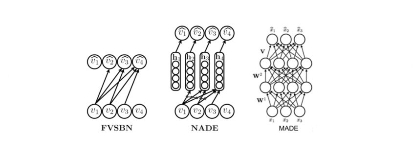
  for the future value prediction. In the other words, autoregressive deep generative models are directed and fully observed models where outcome of the data completely depends on the previous data points as shown in Figure 1.
 , where
  is a set of images and each images is
  dimensional (n pixels). Then the prediction of new data pixel will be depending all the previously predicted pixels (Figure ?? shows the one row of pixels from an image). Referring to our last blog, deep generative models (DGMs) aim to learn the data distribution
  of the given training data and by following the chain rule of the probability, we can express it as:
 random variables. On the other hand, these kind of representation can have exponential space complexity. Therefore, in autoregressive generative models (AGM), these conditionals are approximated/parameterized by neural networks.

 does not depend on
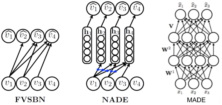


 is known, and
  , given that the state at the time step
  is
is ![v_{\pi} (s)\doteq \mathbb{E}_{\pi} [ G_t | S_t =s ] =\mathbb{E}_{\pi} [ R_{t+1} + \gamma R_{t+2} + \gamma ^2 R_{t+3} + \cdots + \gamma ^{T-t -1} R_{T} |S_t =s]](https://data-science-blog.com/en/wp-content/ql-cache/quicklatex.com-10b9dc282a7d98ce7ecaf0316096f9c9_l3.png "Rendered by QuickLaTeX.com")
 like
like  . But the number
 ![v_{\pi} (s)= \mathbb{E}_{\pi} [ R_{t+1} + \gamma v_{\pi}(S_{t+1}) | S_t =s ]](https://data-science-blog.com/en/wp-content/ql-cache/quicklatex.com-349331e8707784287bb3fd227c4f03af_l3.png "Rendered by QuickLaTeX.com")
 at the left side,
 ![v_{k+1} (s)\doteq \mathbb{E}_{\pi} [ R_{t+1} + \gamma v_{k}(S_{t+1}) | S_t =s ]](https://data-science-blog.com/en/wp-content/ql-cache/quicklatex.com-ba20177dbed44812a6f2ce98154e2c2e_l3.png "Rendered by QuickLaTeX.com")
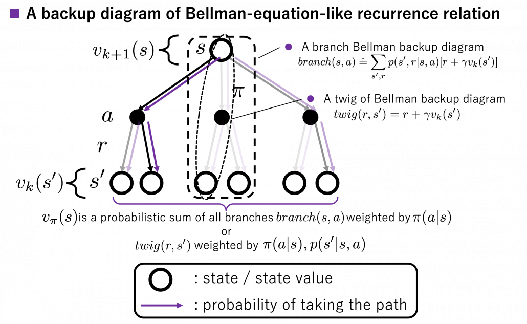
 , namely a probabilistic sum of future rewards is defined as follows.
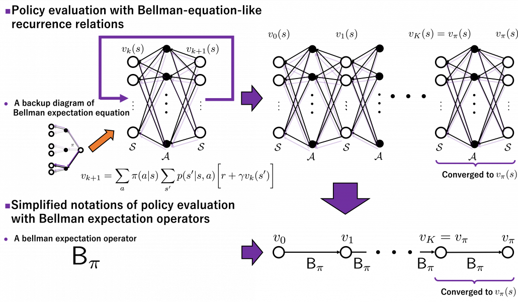
![v_{k+1} (s) = \mathbb{E}_{\pi} [R_{t+1} + \gamma v_k (S_{t+1}) | S_t = s] \doteq \sum_a {\pi(a|s)} \sum_{s', r} {p(s', r|s, a)[r + \gamma v_k(s')]}](https://data-science-blog.com/en/wp-content/ql-cache/quicklatex.com-1a1aa71a4846a76bd8220751fa988103_l3.png "Rendered by QuickLaTeX.com")
 are probabilities of transitions. Policies are probabilities of taking an action
  weighted by
  weighted by
  . “Branches” and “twigs” are terms which I coined.
 is calculated like in the figure below, using values of
  . As I explained earlier, the value of the state
  is a sum of
  . And I showed the weight as strength of purple color of the arrows.
  are corresponding rewards of each transition. And importantly, the Bellman-equation-like operation, whish is a part of DP, is conducted inside the agent. The agent does not have to actually move, and that is what planning is all about.
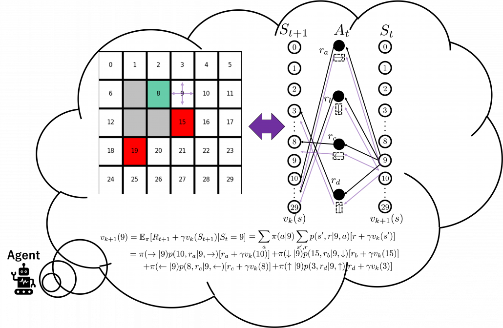
 to
to  . I tried to show the idea that values
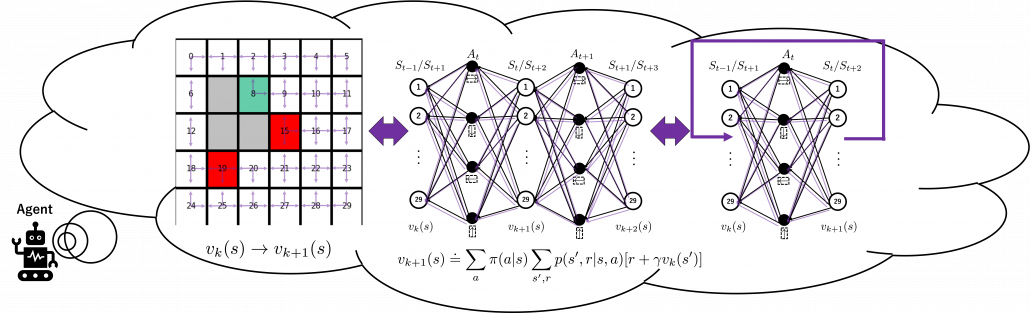
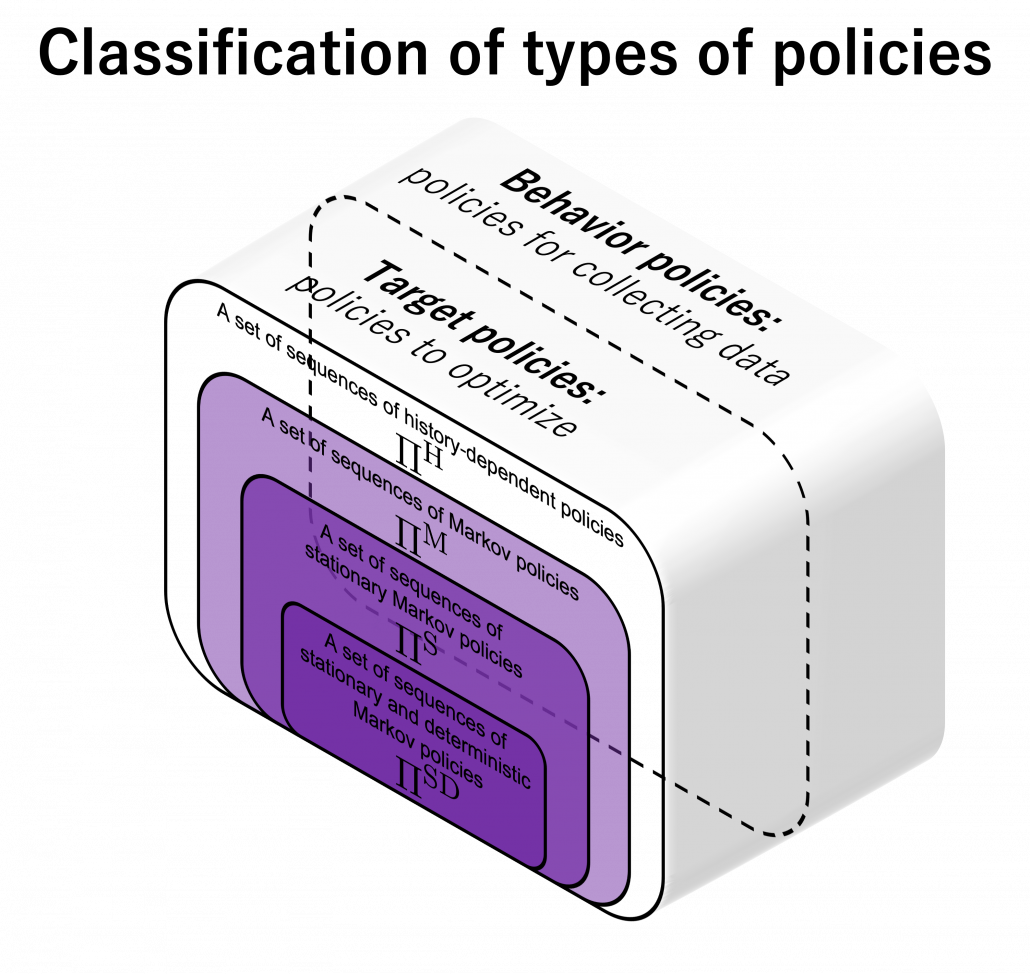
 in the figure below are of interest when you learn RL as a beginner. I am going to explain what each set of policies means one by one.
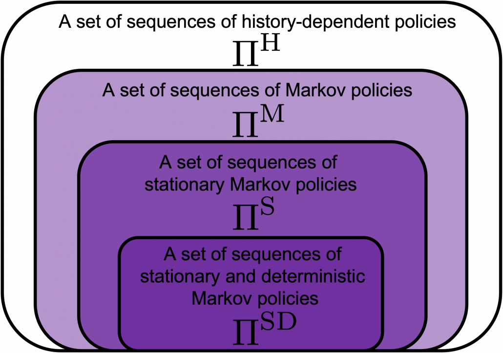
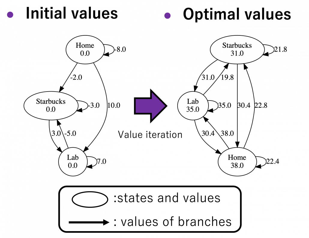
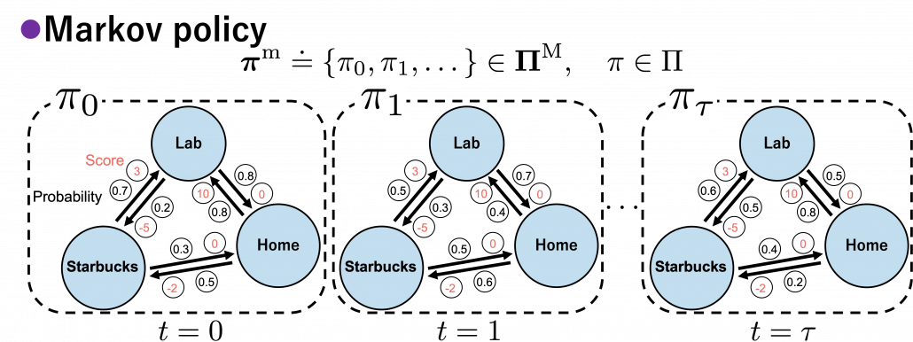
 , which mean probabilistic Markov policies. Remember that in the first article I explained Markov decision processes can be described like diagrams of daily routines. For example, the diagrams below are my daily routines. The indexes
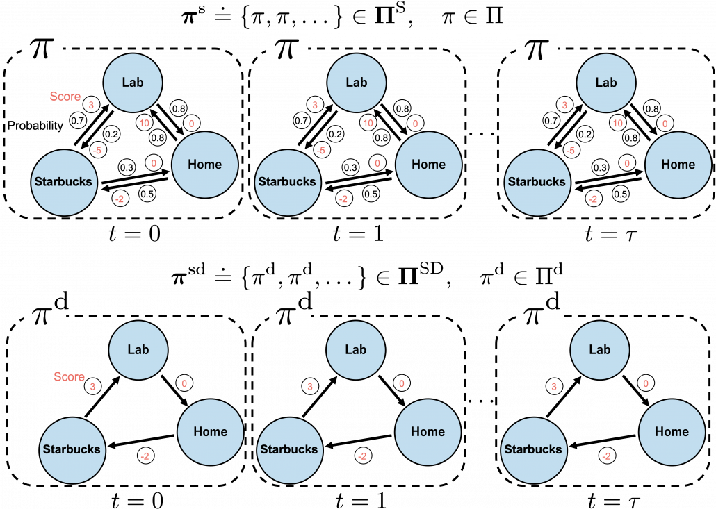
![\Pi \doteq \biggl\{ \pi : \mathcal{A}\times\mathcal{S} \rightarrow [0, 1]: \sum_{a \in \mathcal{A}}{\pi (a|s) =1, \forall s \in \mathcal{S} } \biggr\}](https://data-science-blog.com/en/wp-content/ql-cache/quicklatex.com-9a217cc6d5cfd59e564fd2132620f89f_l3.png "Rendered by QuickLaTeX.com")
 maps any combinations of an action
  and a state
  to a probability. The diagram above means you choose a policy
  , and you use the policy every time step
  . And a set of such stationary Markov policy sequences is denoted as
  .
. are called deterministic policies.
 .
.
 . However as I said, only
  in the context of DP or RL are defined as follows.

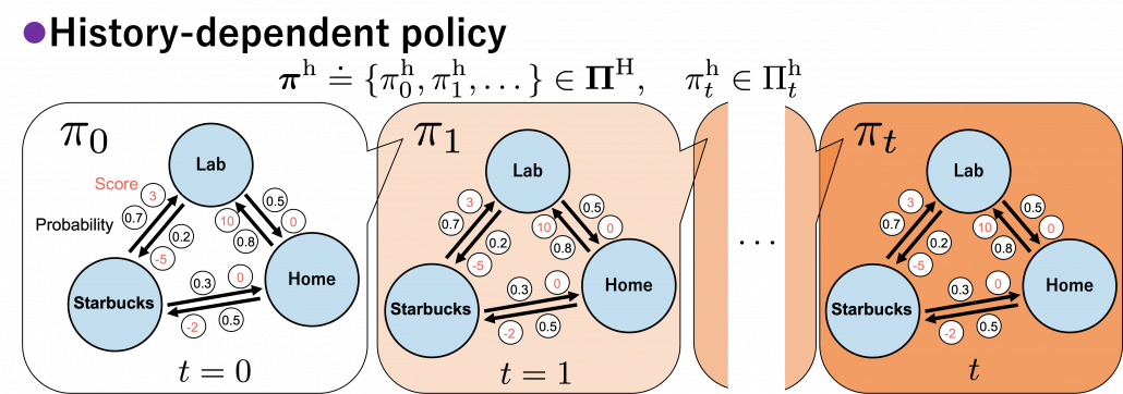
 . It might be more understandable with the graphical model below, which I showed also in the first article. In the graphical model,
  is a random variable, and
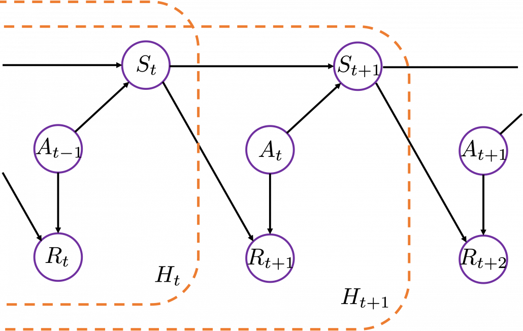
![\Pi _{t}^{\text{h}} \doteq \biggl\{ \pi _{t}^{h} : \mathcal{A}\times\mathcal{H}_t \rightarrow [0, 1]: \sum_{a \in \mathcal{A}}{\pi_{t}^{\text{h}} (a|h_{t}) =1 } \biggr\}](https://data-science-blog.com/en/wp-content/ql-cache/quicklatex.com-6414a4a7c3e4041e14077fce7a8c3fa1_l3.png "Rendered by QuickLaTeX.com")
 .
. or
or  is defined as the maximum value functions for all states
  .
.

 . That means, in the example graphical models I displayed, you just have to deterministically go back and forth between the lab and the home in order to maximize value function, never stopping by at a Starbucks. Also you do not have to change your plans depending on days.
 is defined. But to make things easier for now, let me skip ore precise formulations. Value functions are defined as expectations of rewards with respect to a single policy or a sequence of policies. You have only to keep it in mind that
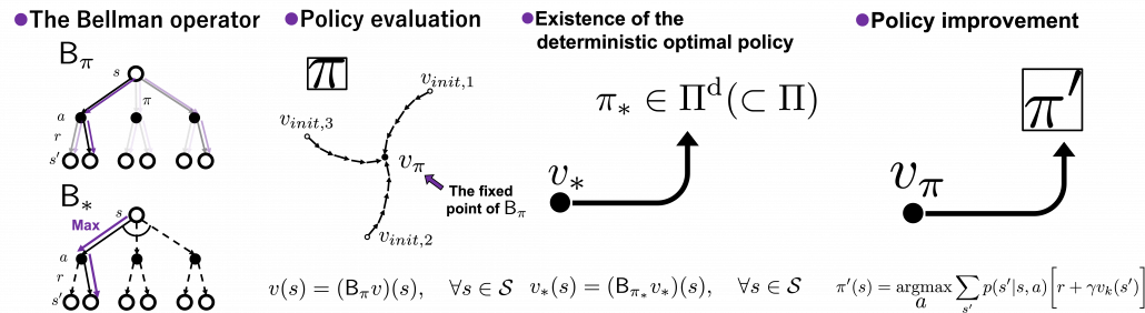
 or
or  .
. , which is deterministic. And it is an optimal policy if and only if it satisfies the Bellman expectation equation
  , with the optimal value function
  .
. , or rather an application of a Bellman expectation operator on any state functions
  is defined as below.
![(\mathsf{B}_{\pi} (v))(s) \doteq \sum_{a}{\pi (a|s)} \sum_{s'}{p(s'| s, a) \biggl[r + \gamma v (s') \biggr]}, \quad \forall s \in \mathcal{S}](https://data-science-blog.com/en/wp-content/ql-cache/quicklatex.com-35022b46d30c7f99c53089770a9dea7e_l3.png "Rendered by QuickLaTeX.com")
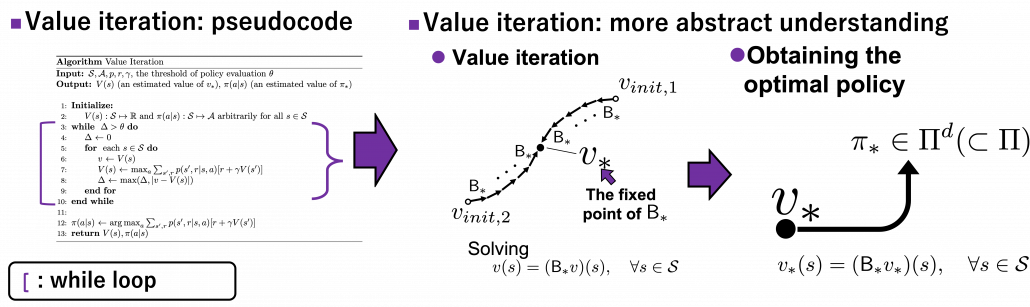
 . In the last article I explained that when
  is an arbitrarily initialized value function, a sequence of value functions
  converge to
 ![v_{k+1} = \sum_{a}{\pi (a|s)} \sum_{s'}{p(s'| s, a) \biggl[r + \gamma v_{k} (s') \biggr]}](https://data-science-blog.com/en/wp-content/ql-cache/quicklatex.com-792e43affeeb5f73e731a3bbd6469f93_l3.png "Rendered by QuickLaTeX.com")

 is obtained by applying
 times in total. Such operation is denoted as follows.
 converges to
 is defined as follows.
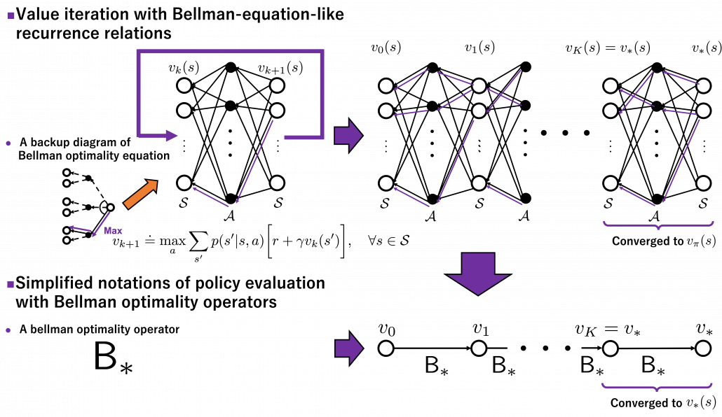
![(\mathsf{B}_{\ast} v)(s) \doteq \max_{a} \sum_{s'}{p(s' | s, a) \biggl[r + \gamma v(s') \biggr]}, \quad \forall s \in \mathcal{S}](https://data-science-blog.com/en/wp-content/ql-cache/quicklatex.com-1c6fc7233a418b4abdfbde6886da4b58_l3.png "Rendered by QuickLaTeX.com")
 . With a Bellman optimality operator, you can get a recurrence relation
  . Multiple applications of Bellman optimality operators can be written down as below.
 converges to the optimal value function
 . If you apply Bellman operators of the policies one by one in an order of
  on a state function
  , the resulting state function is calculated as below.
 , we can also discuss convergence of
  , but that is just confusing. Please let me know if you are interested.
![v(s) = \sum_{a}{\pi (a|s)} \sum_{s'}{p(s'| s, a) \biggl[r + \gamma v (s') \biggr]}](https://data-science-blog.com/en/wp-content/ql-cache/quicklatex.com-d96ea8fd9bc433436f0c1636288df540_l3.png "Rendered by QuickLaTeX.com")
 . But whichever the notation is, the equation holds when the value function
  .
. , and the
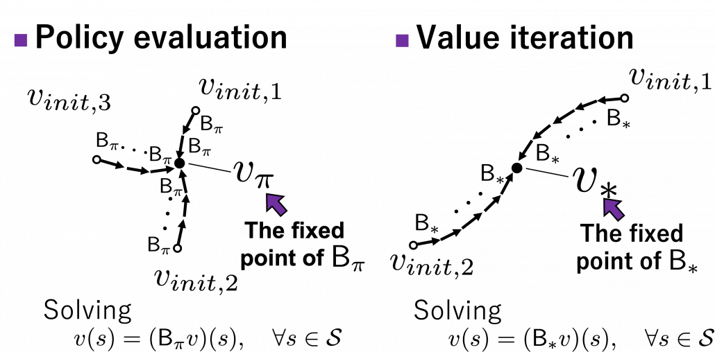
 . And also, you can judge whether a policy is optimal by a Bellman expectation equation below.
![\[v_{\ast}(s) = (\mathsf{B}_{\pi^{\ast} } v_{\ast})(s), \quad \forall s \in \mathcal{S} \]](https://data-science-blog.com/en/wp-content/ql-cache/quicklatex.com-c1a7be583f553c908c51f71b23ea4cff_l3.png "Rendered by QuickLaTeX.com")
![\[\pi^{\text{d}}_{\ast}(s) = \argmax_{a\in \matchal{A}} \sum_{s'}{p(s' | s, a) \biggl[r + \gamma v_{\ast}(s') \biggr]}, \quad \forall s \in \mathcal{S}\]](https://data-science-blog.com/en/wp-content/ql-cache/quicklatex.com-df3b441c33bb9e154ed039a5431676f9_l3.png "Rendered by QuickLaTeX.com")
 . After some calculations,
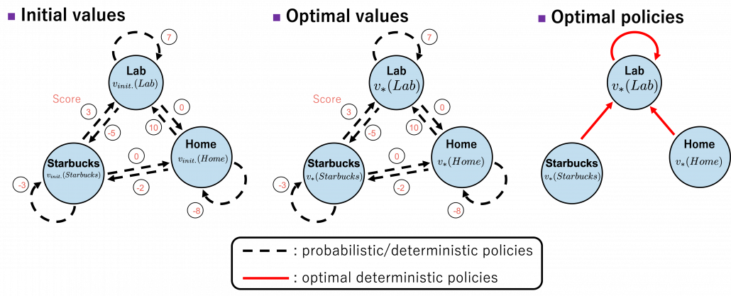
![b(s, a)\doteq\sum_{s'}{p(s' | s, a) \biggl[r + \gamma v_{\ast}(s') \biggr]} = r + \gamma \sum_{s'}{p(s' | s, a) v_{\ast}(s') }](https://data-science-blog.com/en/wp-content/ql-cache/quicklatex.com-cb95afc26ed333c0bc782b865d2595f1_l3.png "Rendered by QuickLaTeX.com") . Let me call the part
. Let me call the part  ” a value of a branch,” and finding the optimal deterministic policy is equal to choosing the maximum branch for all
  and all the all the states
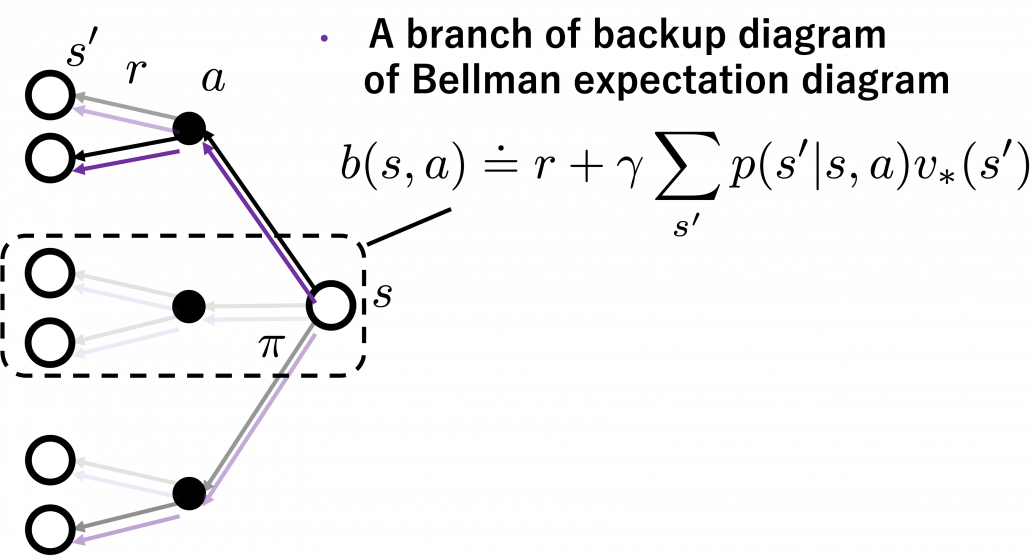
 , and after some iterations they converged to the optimal values. The numbers in each node are values of the sates. And the numbers next to each edge are corresponding values of branches
  . After you get the optimal value, if you choose the direction with the maximum branch at each state, you get the optimal deterministic policy. And that means “Just go to the lab, not Starbucks.”