AI for games, games for AI
1, Who is playing or being played?
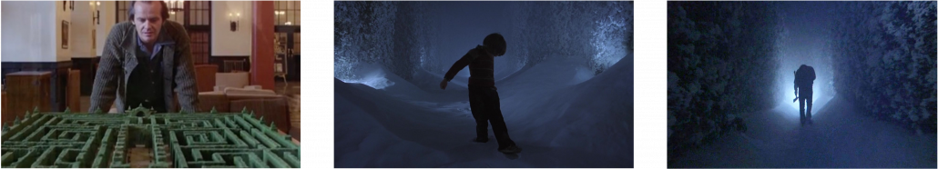
Since playing Japanese video games named “Demon’s Souls” and “Dark Souls” when they were released by From Software, I had played almost no video games for many years. During the period, From Software established one genre named soul-like games. Soul-like games are called 死にゲー in Japanese, which means “dying games,” and they are also called マゾゲー, which means “masochistic games.” As the words imply, you have to be almost masochistic to play such video games because you have to die numerous times in them. And I think recently it has been one of the most remarkable times for From Software because in November of 2021 “Dark Souls” was selected the best video game ever by Golden Joystick Awards. And in the end of last February a new video game by From Software called “Elden Ring” was finally released. After it proved that Miyazaki Hidetaka, the director of Soul series, collaborated with George RR Martin, the author of the original of “Game of Thrones,” “Elden Ring” had been one of the most anticipated video games. In spite of its notorious difficulty as well as other soul-like games so far, “Elden Ring” became a big hit, and I think Miyazak Hidetaka is now the second most famous Miyazaki in the world. A lot of people have been playing it, raging, and screaming. I was no exception, and it took me around 90 hours to finish the video game, breaking a game controller by the end of it. It was a long time since I had been so childishly emotional last time, and I was almost addicted to trial and errors the video game provides. At the same time, one question crossed my mind: is it the video game or us that is being played?
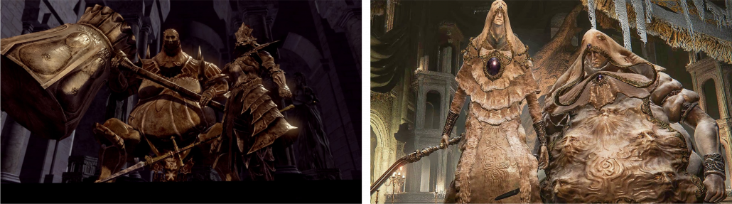
The childhood nightmare strikes back. Left: the iconic and notorious boss duo Ornstein and Smough in Dark Souls (2011), right: Godskin Duo in Elden Ring (2022).
Miyazaki Hidetaka entered From Software in 2004 and in the beginning worked as a programmer of game AI, which controls video games in various ways. In the same year an AI researcher Miyake Youichiro also joined From Software, and I studied a little about game AI by his book after playing “Elden Ring.” I found that he also joined “Demon’s Souls,” in which enemies with merciless game AI were arranged, and I had to conquer them to reach the demon in the end at every dungeon. Every time I died, even in the terminal place with the boss fight, I had to restart from the start, with all enemies reviving. That requires a lot of trial and errors, and that was the beginning of soul-like video games today. In the book by the game AI researcher who was creating my tense and almost traumatizing childhood experiences, I found that very sophisticated techniques have been developed to force players to do trial and errors. They were sophisticated even at a level of controlling players at a more emotional level. Even though I am familiar with both of video games and AI at least more than average, it was not until this year that I took care about this field. After technical breakthroughs mainly made Western countries, video game industry showed rapid progress, and industry is now a huge entertainment industry, whose scale is now bigger that those of movies and music combined. Also the news that Facebook changed its named to Meta and that Microsoft announced to buy Activision Blizzard were sensational recently. However media coverage about those events would just give you impressions that those giant tech companies are making uses of the new virtual media as metaverse or new subscription services. At least I suspect these are juts limited sides of investments on the video game industry.
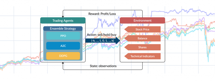
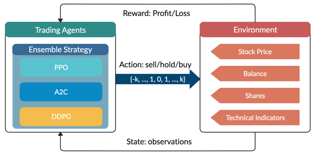
The book on game AI also made me rethink AI technologies also because I am currently writing an article series on reinforcement learning (RL) as a kind of my study note. RL is a type of training of an AI agent through trial-and-error-like processes. Rather than a labeled dataset, RL needs an environment. Such environment receives an action from an agent and gives the consequent state and next reward. From a view point of the agent, it give an action and gets the consequent next state and a corresponding reward, which looks like playing a video game. RL mainly considers a more simplified version of video-game-like environments called a Markov decision processes (MDPs), and in an MDP at a time step  an RL agents takes an action
  , and gets the next state
  and a corresponding reward
  . An MDP is often displayed as a graph at the left side below or the graphical model at the right side.

Compared to a normal labeled dataset used for other machine learning, such environment is something hard to prepare. The video game industry has been a successful manufacturer of such environments, and as a matter of fact video games of Atari or Nintendo Entertainment System (NES) are used as benchmarks of theoretical papers on RL. Such video games might be too primitive for considering practical uses, but researches on RL are little by little tackling more and more complicated video games or simulations. But also I am sure creating AI that plays video games better than us would not be their goals. The situation seems like they are cultivating a form of more general intelligence inside computer simulations which is also effective to the real world. Someday, experiences or intelligence grown in such virtual reality might be dragged to our real world.
Testing systems in simulations has been a fascinating idea, and that is also true of AI research. As I mentioned, video games are frequently used to evaluate RL performances, and there are some tools for making RL environments with modern video game engines. Providing a variety of such sophisticated computer simulations will be indispensable for researches on AI. RL models need to be trained in simulations before being applied on physical devices because most real machines would not endure numerous trial and errors RL often requires. And I believe the video game industry has a potential of developing such experimental fields of AI fueled by commercial success in entertainment. I think the ideas of testing systems or training AI in simulations is getting a bit more realistic due to recent development of transfer learning.
Transfer learning is a subfield of machine learning which apply intelligence or experiences accumulated in datasets or tasks to other datasets or tasks. This is not only applicable to RL but also to more general machine learning tasks like regression or classification. Or rather it is said that transfer learning in general machine learning would show greater progress at a commercial level than RL for the time being. And transfer learning techniques like using pre-trained CNN or BERT is already attracting a lot of attentions. But I would say this is only about a limited type of transfer learning. According to Matsui Kota in RIKEN AIP Data Driven Biomedical Science Team, transfer learning has progressed rapidly after the advent of deep learning, but many types of tasks and approaches are scattered in the field of transfer learning. As he says, the term transfer learning should be more carefully used. I would like to say the type of transfer learning discussed these days are a family of approaches for tackling lack of labels. At the same time some of current researches on transfer learning is also showing possibilities that experiences or intelligence in computer simulations are transferable to the real world. But I think we need to wait for more progress in RL before such things are enabled.
![]()
In this article I would like to explain how video games or computer simulations can provide experiences to the real world in two ways. I am first going to briefly explain how video game industry in the first place has been making game AI to provide game users with tense experiences. And next I will explain how RL has become a promising technique to beat such games which were originally invented to moderately harass human players. And in the end, I am going to briefly introduce ideas of transfer learning applicable to video games or computer simulations. What I can talk in this article is very limited for these huge study areas or industries. But I hope you would see the video game industry and transfer learning in different ways after reading this article, and that might give you some hints about how those industries interact to each other in the future. And also please keep it in mind that I am not going to talk so much about growing video game markets, computer graphics, or metaverse. Here I focus on aspects of interweaving knowledge and experiences generated in simulation or real physical worlds.
2, Game AI
The fact that “Dark Souls” was selected the best game ever at least implies that current video game industry makes much of experiences of discoveries and accomplishments while playing video games, rather than cinematic and realistic computer graphics or iconic and world widely popular characters. That is a kind of returning to the origin of video games. Video games used to be just hard because the more easily players fail, the more money they would drop in arcade games. But I guess this aspect of video games tend to be missed when you talk about video games as a video game fan. What you see in advertisements of video games are more of beautiful graphics, a new world, characters there, and new gadgets. And it has been actually said that qualities of computer graphics have a big correlation with video game sales. In the third article of my series on recurrent neural networks (RNN), I explained how video game industry laid a foundation of the third AI boom during the second AI winter in 1990s. To be more concrete, graphic cards developed rapidly to realize more photo realistic graphics in PC games, and the graphic card used in Xbox was one of the first programmable GPU for commercial uses. But actually video games developed side by side with computer science also outside graphics. Thus in this section I am going to how video games have developed by focusing on game AI, which creates intelligence in video games in several ways. And my explanations on game AI is going to be a rough introduction to a huge and great educational works by Miyake Youichiro.
Playing video games is made up by decision makings, and such decision makings are made in react to game AI. In other words, a display is input into your eyes or sight nerves, and sequential decision makings, that is how you have been moving fingers are outputs. Complication of the experiences, namely hardness of video games, highly depend on game AI. Game AI is mainly used to design enemies in video games to hunt down players. Ideally game AI has to be both rational and human. Rational game AI implemented in enemies frustrate or sometimes despair users by ruining users’ efforts to attack them, to dodge their attacks, or to use items. At the same time enemies have to retain some room for irrationality, that is they have to be imperfect. If enemies can perfectly conquer players’ efforts by instantly recognizing their commands, such video games would be theoretically impossible to beat. Trying to defeat such enemies is nothing but frustrating. Ideal enemies let down their guard and give some timings for attacking and trying to conquer them. Sophisticated game AI is inevitable to make grownups all over the world childishly emotional while playing video games.
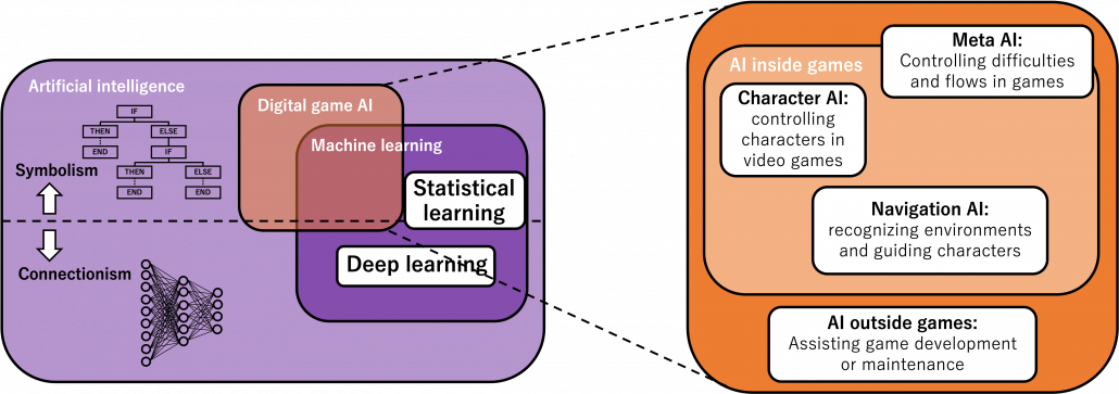
These behaviors of game AI are mainly functions of character AI, which is a part of game AI. In order to explain game AI, I also have to explain a more general idea of AI, which is not the one often called “AI” these days. Artificial intelligence (AI) is in short a family of technologies to create intelligence, with computers. And AI can be divided into two types, symbolism AI and connectionism AI. Roughly speaking, the former is manual and the latter is automatic. Symbolism AI is described with a lot of rules, mainly “if” or “else” statements in code. For example very simply “If the score is greater than 5, the speed of the enemy is 10.” Or rather many people just call it “programming.”
*Note that in contexts of RL, “game AI” often means AI which plays video games or board games. But “game AI” in video games is a more comprehensive idea orchestrating video games.
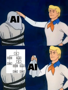
This meme describes symbolism AI well.
What people usually call “AI” in this 3rd AI boom is the latter, connictionism AI. Connectionism AI basically means neural networks, which is said to be inspired by connections of neurons. But the more you study neural networks, the more you would see such AI just as “functions capable of universal approximation based on data.” That means, a function  , which you would have learned in school such as
  is replaced with a complicated black box, and such black box is automatically learned with many combinations of
  . And such black boxes are called neural networks, and the combinations of datasets. Connectionism AI might sound more ideal, but in practice it would be hard to design characters in AI based on such training with datasets.
*Connectionism, or deep learning is of course also programming. But in deep learning we largely depend on libraries, and a lot of parameters of AI models are updated automatically as long as we properly set datasets. In that sense, I would connectionism is more automatic. As I am going to explain, game AI largely depends on symbolism AI, namely manual adjustment of lesser parameters, but such symbolism AI would behave much more like humans than so called “AI” these days when you play video games.
Digital game AI today is application of the both types of AI in video games. It initially started mainly with symbolism AI till around 2010, and as video games get more and more complicated connectionism AI are also introduced in game AI. Video game AI can be classified to mainly navigation AI, character AI, meta AI, procedural AI, and AI outside video games. The figure below shows relations of general AI and types of game AI.
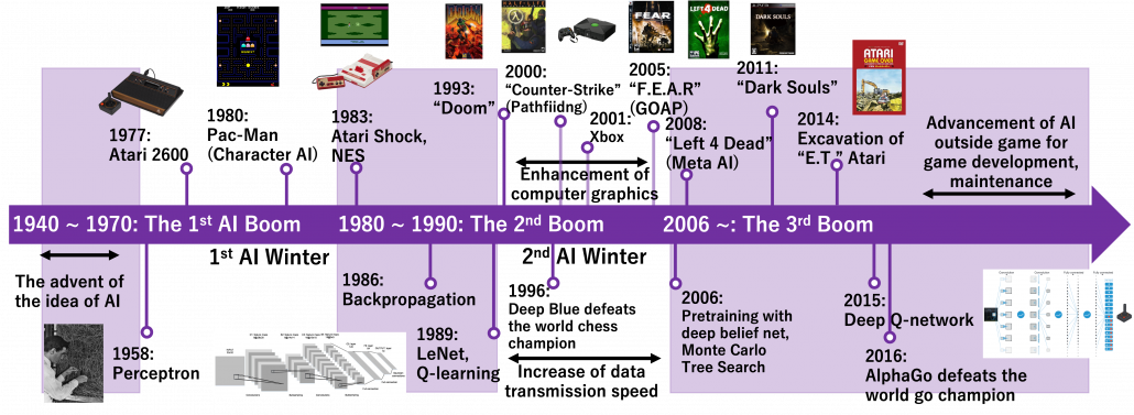
Very simply putting, video game AI traced a history like this: the initial video games were mainly composed of navigation AI showing levels, maps, and objects which move deterministically based on programming. Players used to just move around such navigation AI. Sooner or later, enemies got certain “intelligence” and learned to chase or hunt down players, and that is the advent of character AI. But of course such “intelligence” is nothing but just manual programs. After rapid progress of video games and their industry, meta AI was invented to control difficulties of video games, thereby controlling players’ emotions. Procedural AI automatically generates contents of video games, so video games are these days becoming more and more massive. And as modern video games are too huge and complicated to debug or maintain manually, AI technologies including deep learning are used. The figure below is a chronicle of development of video games and AI technologies covered in this article. Let’s see a brief history of video games and game AI by taking a closer look at each type of game AI a little more precisely.
Navigation AI
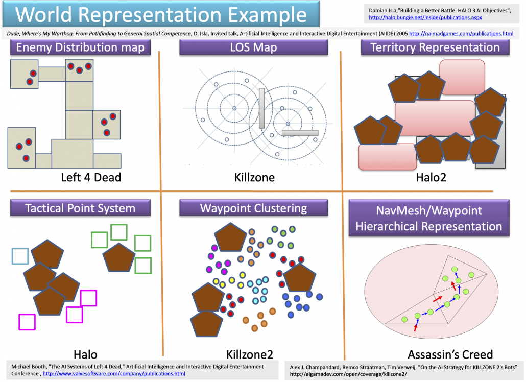
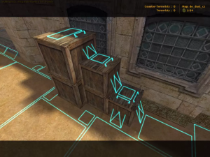
Navigation AI is the most basic type of game AI, and that allows character AI to recognize the world in video games. Even though I think character AI, which enables characters in video games to behave like humans, would be the most famous type of game AI, it is said navigation AI has an older history. One important function of navigation AI is to control objects in video games, such as lifts, item blocks, including attacks by such objects. The next aspect of navigation AI is that it provides character AI with recognition of worlds. Unlike humans, who can almost instantly roughly recognize circumstances, character AI cannot do that as we do. Even if you feel as if the character you are controlling are moving around mountains, cities, or battle fields, sometimes escaping from attacks by other AI, for character AI that is just moving on certain graphs. The figure below are some examples of world representations adopted in some popular video games. There are a variety of such representations, and please let me skip explaining the details of them. An important point is, relatively wide and global recognition of worlds by characters in video games depend on how navigation AI is designed.
The next important feature of navigation AI is path finding. If you have learned engineering or programming, you should be already familiar with pathfiniding algorithms. They had been known since a long time ago, but it was not until “Counter-Strike” in 2000 the techniques were implemented at an satisfying level for navigating characters in a 3d world. Improvements of pathfinding in video games released game AI from fixed places and enabled them to be more dynamic.
*According to Miyake Youichiro, the advent of pathfinding in video games released character AI from staying in a narrow space and enable much more dynamic and human-like movements of them. And that changed game AI from just static objects to more intelligent entity.
Navigation meshes in “Counter-Strike (2000).” Thanks to these meshes, continuous 3d world can be processed as discrete nodes of graphs.
Character AI
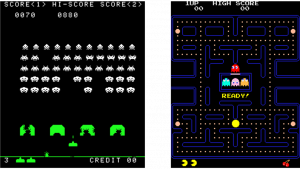
Character AI is something you would first imagine from the term AI. It controls characters’ actions in video games. And differences between navigation AI and character AI can be ambiguous. It is said Pac-Man is one of the very first character AI. Compared to aliens in Space Invader deterministically moved horizontally, enemies in Pac-Man chase a player, and this is the most straightforward difference between navigation AI and character AI.
Character AI is a bunch of sophisticated planning algorithms, so I can introduce only a limited part of it just like navigation AI. In this article I would like to take an example of “F.E.A.R.” released in 2005. It is said goal-oriented action planning (GOAP) adopted in this video game was a breakthrough in character AI. GOAP is classified to backward planning, and if there exists backward ones, there is also forward ones. Using a game tree is an examples of forward planning. The figure below is an example of a tree game of tic-tac-toe. There are only 9 possible actions at maximum at each phase, so the number of possible states is relatively limited.

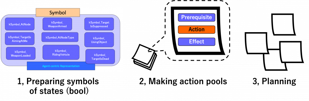
But with more options of actions like most of video games, forward plannings have to deal much larger sizes of future action combinations. GOAP enables realistic behaviors of character AI with a heuristic idea of planning backward. To borrow Miyake Youichiro’s expression, GOAP processes actions like sticky notes. On each sticky note, there is a combination of symbols like “whether a target is dead,” “whether a weapon is armed,” or “whether the weapon is loaded.” A sticky note composed of such symbols form an action, and each action comprises a prerequisite, an action, and an effect. And behaviors of character AI is conducted with planning like pasting the sticky notes.
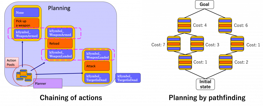
 More practically sticky notes, namely actions are stored in actions pools. For a decision making, as displayed in the left side of the figure below, actions are connected as a chain. First an action of a goal is first set, and an action can be connected to the prerequisite of the goal via its effect. Just as well corresponding former actions are selected until the initial state. In the example of chaining below, the goal is “kSymbol_TargetIsDead,” and actions are chained via “kSymbol_TargetIsDead,” “kSymbol_WeaponLoaded,” “kSymbol_WeaponArmed,” and “None.” And there are several combinations of actions to reach a certain goal, so more practically each action has a cost, and the most ideal behavior of character AI is chosen by pathfinding on a graph like the right side of the figure below. And the best planning is chosen by a pathfinding algorithm.
Even though many of highly intelligent behaviors of character AI are implemented as backward plannings as I explained, planning forward can be very effective in some situations. Board game AI is a good example. A searching algorithm named Monte Carlo tree search is said to be one breakthroughs in board game AI. The searching algorithm randomly plays a game until the end, which is called playout. Numerous times of playouts enables evaluations of possibilities of winning. Monte Carlo Tree search also enables more efficient searches of games trees.
Meta AI
Meta AI is a type of AI such that controls a whole video game to enhance player’s experiences. To be more concrete, it adjusts difficulties of video games by for example dynamically arranging enemies. I think differences between meta AI and navigation AI or character AI can be also ambiguous. As I explained, the earliest video games were composed mainly with navigation AI, or rather just objects. Even if there are aliens or monsters, they can be just part of interactive objects as long as they move deterministically. I said character AI gave some diversities to their behaviors, but how challenging a video game is depends on dynamic arrangements of such objects or enemies. And some of classical video games like “Xevious,” as a matter of fact implemented such adjustments of difficulties of game plays. That is an advent of meta AI, but I think they were not so much distinguished from other types of AI, and I guess meta AI has been unconsciously just a part of programming.
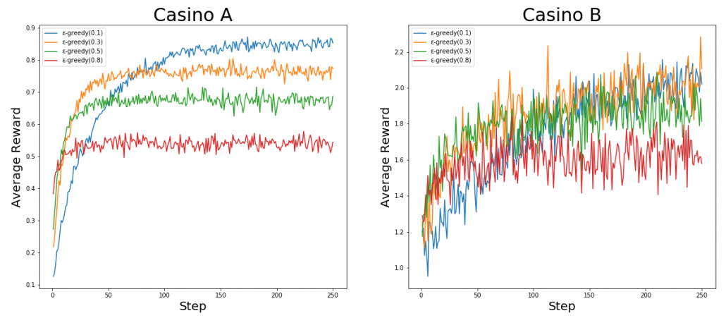
It is said a turning point of modern meta AI is a shooting game “Left 4 Dead” released in 2008, where zombies are dynamically arranged. As well as many masterpiece thriller films, realistic and tense terrors are made by combinations of intensities and relaxations. Tons of monsters or zombies coming up one after another and just shooting them look stupid or almost like comedies. .And analyzing the success of “Counter-Strike,” they realized that users liked rhythms of intensity and relaxation, so they implemented that explicitly in “Left 4 Dead.” The graphs below concisely shows how meta AI works in the video game. When the survivor intensity, namely players’ intensity is low, the meta AI arrange some enemies. Survivor intensity increases as players fight with zombies or something, and then meta AI places fewer enemies so that players can relax. While players re relatively relaxing, desired population of enemies increases when they actually show up in video games, again the phase of intensity comes.
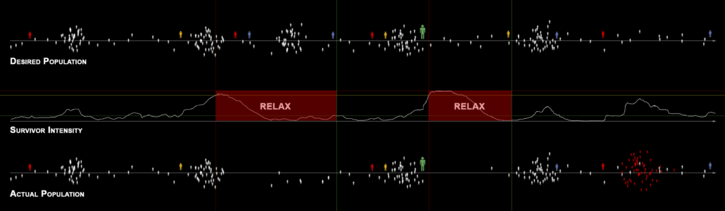
*Soul series video games do not seem to use meta AI so much. Characters in the games are rearranged in more or less the same ways every time players fail. Soul-like games make much of experiences that players find solutions by themselves, which means that manual but very careful arrangements of enemies and interactive objects are also very effective.
Meta AI can be used to make video games more addictive using data analysis. Recent social network games can record logs of game plays. Therefore if you can observe a trend that more users unsubscribe when they get less rewards in certain online events, operating companies of the game can adjust chances of getting “rare” items.
Procedural AI and AI outside video games
How clearly you can have an image of what I am going to explain in this subsection would depend how recently you have played video games. If your memories of playing video games stops with good old days of playing side-scrolling ones like Super Mario Brothers, you should at first look up some videos of playing open world games. Open world means a use of a virtual reality in which players can move an behave with a high degree of freedom. The term open world is often used as opposed to the linear games, where players have process games in the order they are given. Once you are immersed in photorealistic computer graphic worlds in such open world games, you would soon understand why metaverse is attracting attentions these days. Open world games for example like “Fallout 4” are astonishing in that you can even talk to almost everyone in them. Just as “Elden Ring” changed former soul series video games into an open world one, it seems providing open world games is one way to keep competitive in the video game industry. And such massive world can be made also with a help of procedural AI. Procedural AI can be seen as a part of meta AI, and it generates components of games such as buildings, roads, plants, and even stories. Thanks to procedural AI, video game companies with relatively small domestic markets like Poland can make a top-level open world game such as “The Witcher 3: Wild Hunt.”

An example of technique of procedural AI adopted in “The Witcher 3: Wild Hunt” for automatically creating the massive open world.
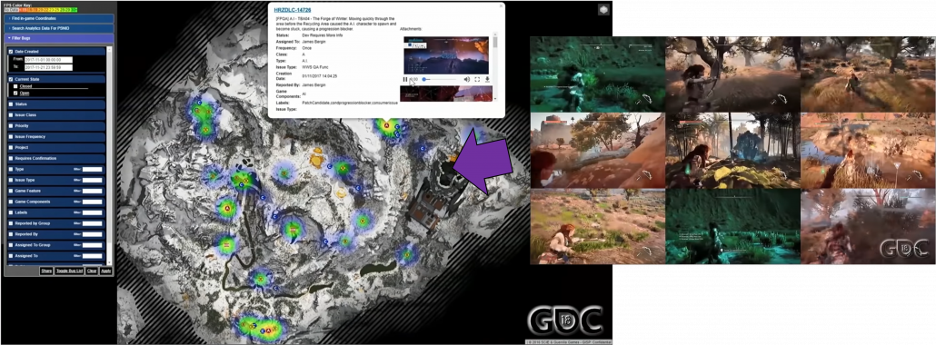
Creating a massive world also means needs of tons of debugging and quality assurance (QA). Combining works by programmers, designers, and procedural AI will cause a lot of unexpected troubles when it is actually played. AI outside game can be used to find these problems for quality assurance. Debugging and and QA have been basically done manually, and especially when it comes to QA, video game manufacturer have to employ a lot of gamer to let them just play prototype of their products. However as video games get bigger and bigger, their products are not something that can be maintained manually anymore. If you have played even one open world game, that would be easy to imagine, so automatic QA would remain indispensable in the video game industry. For example an open world game “Horizon Zero Dawn” is a video game where a player can very freely move around a massive world like a jungle. The QA team of this video game prepared bug maps so that they can visualize errors in video games. And they also adopted a system named “Apollo-Autonomous Automated Autobots” to let game AI automatically play the video game and record bugs.
As most video games both in consoles or PCs are connected to the internet these days, these bugs can be fixed soon with updates. In addition, logs of data of how players played video games or how they failed can be stored to adjust difficulties of video games or train game AI. As you can see, video games are not something manufacturers just release. They are now something develop interactively between users and developers, and players’ data is all exploited just as your browsing history on the Internet.
I have briefly explained AI used for video games over four topics. In the next two sections, I am going to explain how board games and video games can be used for AI research.
3, Reinforcement learning: we might be a sort of well-made game AI models
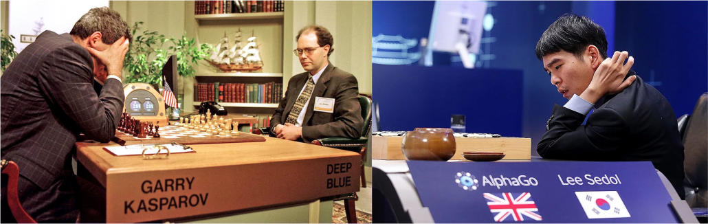
Machine learning, especially RL is replacing humans with computers, however with incredible computation resources. Invention of game AI, in this context including computers playing board games, has been milestones of development of AI for decades. As Western countries had been leading researches on AI, defeating humans in chess, a symbol of intelligence, had been one of goals. Even Alan Turing, one of the fathers of computers, programmed game AI to play chess with one of the earliest calculators. Searching algorithms with game trees were mainly studied in the beginning. Game trees are a type of tree graphs to show how games proceed, by expressing future possibilities with diverging tree structures. And searching algorithms are often used on tree graphs to ignore future steps which are not likely to be effective, which often looks like cutting off branches of trees. As a matter of fact, chess was so “simple” that searching algorithms alone were enough to defeat Garry Kasparov, the world chess champion at that time in 1997. That is, growing trees and trimming them was enough for the “simplicity” of chess as long as a super computer of IBM was available. After that computer defeated one of the top players of shogi, a Japanese version of chess, in 2013. And remarkably, in 2016 AlphaGo of DeepMind under Google defeated the world go champion. Game AI has been gradually mastering board games in order of increasing search space size.
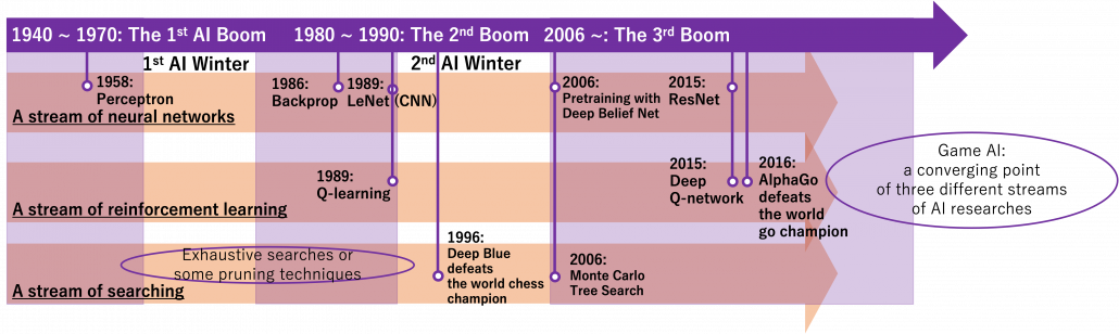
We can say combinations of techniques which developed in different streams converged into game AI today, like I display in the figure below. In AlphaGo or maybe also general game AI, neural networks enable “intuition” on phases of board games, searching algorithms enables “foreseeing,” and RL “experiences.” And as almost no one can defeat computers in board games anymore, the next step of game AI is how to conquer other video games. Since progress of convolutional neural network (CNN) in this 3rd AI boom, computers got “eyes” like we do, and the invention of ResNet in 2015 is remarkable. Thus we can now use displays of video games as inputs to neural networks. And combinations of reinforcement learning and neural networks like (CNN) is called deep reinforcement learning. Since the advent of deep reinforcement learning, many people are trying to apply it on various video games, and they show impressive results. But in general that is successful in bird’s-eye view games. Even if some of researches can be competitive or outperform human players, even in first person shooting video games, they require too much computational resources and heuristic techniques. And usually they take too much time and computer resource to achieve the level.
*Even though CNN is mainly used as “eyes” of computers, it is also used to process a phase of a board game. That means each phase of is processed like an arrangement of pixels of an image. This is what I mean by “intuition” of deep learning. Just as neural networks can recognize objects, depending on training methods they can recognize boards at a high level.
Now I would like you to think about what “smartness” means. Competency in board games tend to have correlations with mathematical skills. And actually in many cases people proficient in mathematics are also competent in board games. Even though AI can defeat incredibly smart top board game players to the best of my knowledge game AI has yet to play complicated video games with more realistic computer graphics. As I explained, behaviors of character AI is in practice implemented as simpler graphs, and tactics taken in such graphs will not be as complicated as game trees of competitive board games. And the idea of game AI playing video games itself not new, and it is also used in debugging of video games. Thus the difficulties of computers playing video games would come more from how to associate what they see on displays with more long-term and more abstract plannings. And currently, kids would more flexibly switch to other video games and play them more professionally in no time. I would say the difference is due to frames of tasks. A frame roughly means a domain or a range which is related to a task. When you play a board game, its frame is relatively small because everything you can do is limited in the rule of the game which can be expressed as simple data structure. But playing video games has a wider frame in that you have to recognize only the necessary parts important for playing video games from its constantly changing displays, namely sequences of RGB images. And in the real world, even a trivial action like putting a class on a table is selected from countless frames like what your room looks like, how soft the floor is, or what the temperature is. Human brains are great in that they can pick up only necessary frames instantly.
As many researchers would already realize, making smaller models with lower resources which can learn more variety of tasks is going to be needed, and it is a main topic these days not only in RL but also in other machine learning. And to be honest, I am skeptical about industrial or academic benefits of inventing specialized AI models for beating human players with gigantic computation resources. That would be sensational and might be effective for gathering attentions and funds. But as many AI researchers would already realize, inventing a more general intelligence which would more flexibly adjust to various tasks is more important. Among various topics of researches on the problem, I am going to pick up transfer learning in the next section, but in a more futuristic and dreamy sense.
4, Transfer learning and game for AI
In an event with some young shogi players, to a question “What would you like to request to a god?” Fujii Sota, the youngest top shogi player ever, answered “If he exists, I would like to ask him to play a game with me.” People there were stunned by the answer. The young genius, contrary to his sleepy face, has an ambition which only the most intrepid figures in mythology would have had. But instead of playing with gods, he is training himself with game AI of shogi. His hobby is assembling computers with high end CPUs, whose performance is monstrous for personal home uses. But in my opinion such situation comes from a fact that humans are already a kind of well-made machine learning models and that highly intelligent games for humans have very limited frames for computers.
*It seems it is not only computers that need huge energy consumption to play board games. Japanese media often show how gorgeous and high caloric shogi players’ meals are during breaks. And more often than not, how fancy their feasts are is the only thing most normal spectators like me in front of TVs can understand, albeit highly intellectual tactics made beneath the wooden boards.
As I have explained, the video game industry has been providing complicated simulational worlds with sophisticated ensemble of game AI in both symbolism and connectionism ways. And such simulations, initially invented to hunt down players, are these days being conquered especially by RL models, and the trend showed conspicuous progress after the advent of deep learning, that is after computers getting “eyes.” The next problem is how to transfer the intelligence or experiences cultivated in such simulations to the real world. Only humans can successfully train themselves with computer simulations today as far as I know, but more practically it is desired to transfer experiences with wider frames to more inflexible entities like robots. Such technologies would be ideal especially for RL because physical devices cannot make numerous trial and errors in the real world. They should be trained in advance in computer simulations. And transfer learning could be one way to take advantages of experiences in computer simulations to the real world. But before talking about such transfer learning, we need to be careful about the term “transfer learning.” Transfer learning is a family of machine learning technologies to makes uses of knowledge learned in a dataset, which is usually relatively huge, to another task with another dataset. Even though I have been emphasizing transferring experiences in computer simulations, transfer learning is a more general idea applicable to more general use cases, also outside computer simulations. Or rather, transfer learning is attracting a lot of attentions as a promising technique for tackling lack of data in general machine learning. And another problem is even though transfer learning has been rapidly developing recently, various research topics are scattered in the field called “transfer learning.” And arranging these topics would need extra articles or something. Thus in the rest of this article, I would like to especially focus on uses of video games or computer simulations in transfer learning. When it comes to already popular and practical transfer learning techniques like fine tuning with pre-trained backbone CNN or BERT, I am planning to cover them with more practical introduction in one of my upcoming articles. Thus in this article, after simply introducing ideas of domains and transfer learning, I am going to briefly introduce transfer learning and explain domain adaptation/randomization.
Domain and transfer learning
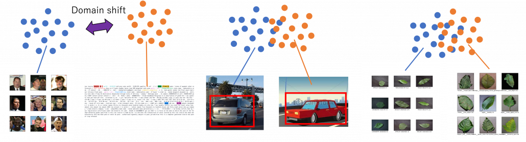
There is a more strict definition of a domain in machine learning, but all you have to know is it means in short a type of dataset used for a machine learning task. And different domains have a domain shift, which in short means differences in the domains. A text dataset and an image dataset have a domain shift. An image dataset of real objects and one with cartoon images also have a smaller domain shift. Even differences in lighting or angles of cameras would cause a domain shift. In general, even if a machine learning model is successful in tasks in a domain, even a domain shift which is trivial to humans declines performances of the model. In other words, intelligence learned in one domain is not straightforwardly applicable to another domain as humans can do. That is, even if you can recognize objects both a real and cartoon cars as a car, that is not necessarily true of machine learning models. As a family of techniques for tackling this problem, transfer learning makes a use of knowledge in a source domain (the dots in blue below), and apply the knowledge to a target domain. And usually, a source domain is assumed to be large and labeled, and on the other hand a target domain is assumed to be relatively small or even unlabeled. And tasks in a source or a target domain can be different. For example, CNN models trained on classification of ImageNet can be effectively used for object detection. Or BERT is trained on a huge corpus in a self-supervised way, but it is applicable to a variety of tasks in natural language processing (NLP).
*To people in computer vision fields, an explanation that BERT is a NLP version of pre-trained CNN would make the most sense. Just as a pre-trained CNN maps an image, arrangements of RGB pixels values, to a vector representing more of “meaning” of the image, BERT maps a text, a sequence of one-hot encodings, into a vector or a sequence of vectors in a semantic field useful for NLP.
Transfer learning is a very popular topic, and it is hard to arrange and explain types of existing techniques. I think that is because many people are tackling more or less the similar problems with slightly different approaches. For now I would like you to keep it in mind that there are roughly three points below to consider in transfer learning
- What to transfer
- When to transfer
- How to transfer
The answer of the second point above “When to transfer” is simply “when domains are more or less alike.” Transfer learning assume similarities between target and source domains to some extent. “How to transfer” is very task-specific, so this is not something I can explain briefly here. I think the first point “what to transfer” is the most important for now to avoid confusions about what “transfer learning” means. “What to transfer” in transfer learning is also classified to the three types below.
- Instance transfer (transferring datasets themselves)
- Feature transfer (transferring extracted features)
- Parameter transfer (transferring pre-trained models)
In fact, when you talk about already practical transfer learning techniques like using pre-trained CNN or BERT, they refer to only parameter transfer above. And please let me skip introducing it in this article. I am going to focus only on techniques related to video games in this article.
*I would like to give more practical introduction on for example BERT in one of my upcoming articles.
Domain adaptation or randomization
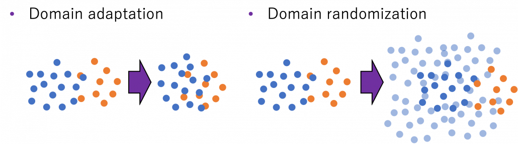
I first got interested in relations of video games and AI research because I was studying domain adaptation, which tackles declines of machine learning performance caused by a domain shift. Domain adaptation is sometimes used as a synonym to transfer learning. But compared to that general transfer learning also assume different tasks in different domains, domain adaptation assume the same task. Thus I would say domain adaptation is a subfield of transfer learning. There are several techniques for domain adaptation, and in this article I would like to take feature alignment as an example of frequently used approaches. Input datasets have a certain domain shift like blue and circle dots in the figure below. This domain shift cannot be changed if datasets themselves are not directly converted. Feature alignment make the domain shift smaller in a feature space after data being processed by the feature extractor. The features expressed as square dots in the figure are passed to task-specific networks just as normal machine learning. With sufficient labels in the source domain and with fewer or no labels in the target one, the task-specific networks are supervised. On the other hand, the features are also passed to the domain discriminator, and the discriminator predicts which domain the feature comes from. The domain discriminator is normally trained with supervision by classification loss, but the feature supervision is reversed when it trains the feature extractor. Due to the reversed supervision the feature extractor learns mix up features because that is worse for discriminating distinguishing the source or target domains. In this way, the feature extractor learns extract domain invariant features, that is more general features both domains have in common.
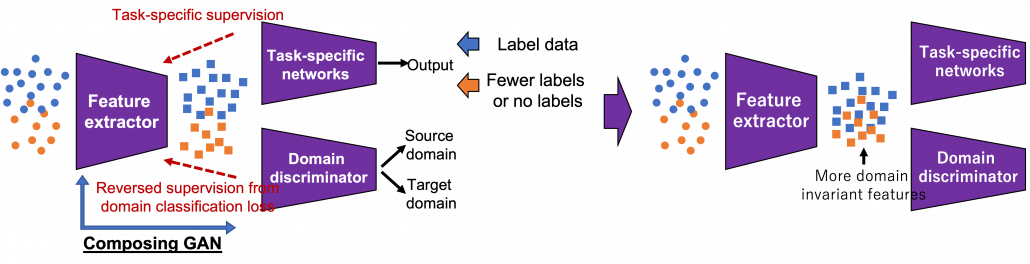
*The feature extractor and the domain discriminator is in a sense composing generative adversarial networks (GAN), which is often used in data generation. To know more about GAN, you could check for example this article.
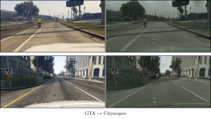
One of motivations behind domain adaptation is that it enables training AI tasks with synthetic datasets made by for example computer graphics because they are very easy to annotate and prepare labels necessary for machine learning tasks. In such cases, domain invariant features like curves or silhouettes are expected to learn. And learning computer vision tasks from GTA5 dataset which are applicable to Cityscapes dataset is counted as one of challenging tasks in papers on domain adaptation. GTA of course stands for “Grand Theft Auto,” the video open-world video game series. If this research continues successfully developing, that would imply possibilities of capability of teaching AI models to “see” only with video games. Imagine that a baby first learns to play Grand Theft Auto 5 above all and learns what cars, roads, and pedestrians are. And when you bring the baby outside, even they have not seen any real cars, they point to a real cars and people and say “car” and “pedestrians,” rather than “mama” or “dada.”
In order to enable more effective domain adaptation, Cycle GAN is often used. Cycle GAN is a technique to map texture in one domain to another domain. The figure below is an example of applying Cycle GAN on GTA5 dataset and Cityspaces Dataset, and by doing so shiny views from a car in Los Santos can be converted to dark and depressing scenes in Germany in winter. This instance transfer is often used in researches on domain adaptation.
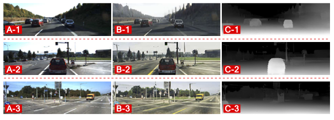
Even if you mainly train depth estimation with data converted like above, the model can predict depth data of the real world domain without correct depth data. In the figure below, A is the target real data, B is the target domain converted like a source domain, and C is depth estimation on A.
Crowd counting is another field where making a labeled dataset with video games is very effective. A MOD for making a crowd arbitrarily is released, and you can make labeled datasets like below.

*Introducing GTA mod into research is hilarious. You first need to buy PC software of Grand Theft Auto 5 and gaming PC at first. And after finishing the first tutorial in the video game, you need to find a place to place a camera, which looks nothing but just playing video games with public money.
Domain adaptation problems I mentioned are more of matters of how to let computers “see” the world with computer simulations. But the gap between the simulational worlds and the real world does not exist only in visual ways like in CV. How robots or vehicles are parametrized in computers also have some gaps from the real world, so even if you replace only observations with simulations, it would be hard to train AI. But surprisingly, some researches have already succeeded in training robot arms only with computer simulations. An approach named domain randomization seems to be more or less successful in training robot arms only with computer simulations and apply the learned experience to the real world. Compared to domain adaptation aligned source domain to the target domain, domain randomization is more of expanding the source domain by changing various parameters of the source domain. And the target domain, namely robot arms in the real world is in the end included in the expanded source domain. And such expansions are relatively easy with computer simulations.
For example a paper “Closing the Sim-to-Real Loop: Adapting Simulation Randomization with Real World Experience” proposes a technique to reflect real world feed back to simulations in domain randomization, and this pipeline enables a robot arm to do real world tasks in a few iteration of real world trainings.

As the video shows, the ideas of training a robot with computer simulations is becoming more realistic.
The future of games for AI
I have been emphasizing how useful video games are in AI researches, but I am not sure if how much the field purely rely on video games like it is doing especially on RL. Autonomous driving is a huge research field, and modern video games like Grand Thef Auto are already good driving simulations in urban areas. But other realistic simulations like CARLA have been developed independent of video games. And in a paper “Exploring the Limitations of Behavior Cloning for Autonomous Driving,” some limitations of training self-driving cars in the simulation are reported. And some companies like Waymo switched to recurrent neural networks (RNN) for self-driving cars. It is natural that fields like self-driving, where errors of controls can be fatal, are not so optimistic about adopting RL for now.
But at the same time, Microsoft bought a Project Bonsai, which is aiming at applying RL to real world tasks. Also Microsoft has Project Malmo or AirSim, which respectively use Minecraft or Unreal Engine for AI reseraches. Also recently the news that Microsoft bought Activision Blizzard was a sensation last year, and media’s interests were mainly about metaverse or subscription service of video games. But Microsoft also bouth Zenimax Media, is famous for open world like Fallout or Skyrim series. Given that these are under Microsoft, it seems the company has been keen on merging AI reserach and developing video games.
As I briefly explained, video games can be expanded with procedural AI technologies. In the future AI might be trained in video game worlds, which are augmented with another form of AI. Combinations of transfer learning and game AI might possibly be a family of self-supervising technologies, like an octopus growing by eating its own feet. At least the biggest advantage of the video game industry is, even technologies themselves do not make immediate profits, researches on them are fueled by increasing video game fans all over the world. This is a kind of my sci-fi imagination of the world. Though I am not sure which is more efficient to manually design controls of robots or training AI in such indirect ways. And I prefer to enhance physical world to metaverse. People should learn to put their controllers someday and to enhance the real world. Highly motivated by “Elden Ring” I wrote this article. Some readers might got interested in the idea of transferring experiences in computer simulations to the real world. I am also going to write about transfer learning in general that is helpful in practice.
* I make study materials on machine learning, sponsored by DATANOMIQ. I do my best to make my content as straightforward but as precise as possible. I include all of my reference sources. If you notice any mistakes in my materials, including grammatical errors, please let me know (email: yasuto.tamura@datanomiq.de). And if you have any advice for making my materials more understandable to learners, I would appreciate hearing it.


 in an state space
  , and black nodes representing each action
  , which is a member of an action space
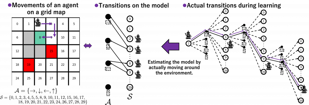
  . Any behaviors of agents are represented as going back and forth between black and white nodes of the model, and that is why connections in the MDP model are bidirectional. In my articles let me call such model of environments “a closed model.” RL or general planning problems are matters of optimizing policies in such models of environments. Optimizing the policies are roughly classified into two types, planning/searching or RL, and the main difference between them is whether connections of graphs of models are known or not. Planning or searching is conducted without actually moving in the environment. DP are family of planning algorithms which are known to converge, and so far in my articles we have seen that DP are enabled by repeatedly applying Bellman operators. But instead of considering and updating all the possible transitions in the model like DP, planning can be conducted more sparsely. Such sparse planning are often called searching, and many of them use tree structures. If you have learned any general decision making problems with tree graphs, you might be already familiar with some searching techniques like alpha-beta pruning.

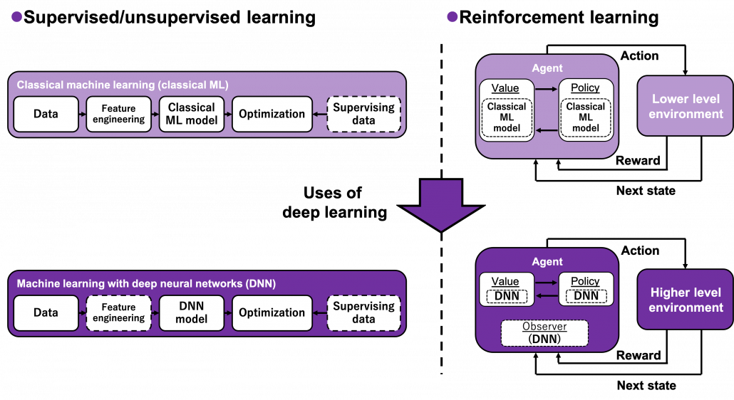
 , in MDPs. Other general machine learning algorithms have more direct supervision by loss functions and models are optimized so that loss functions are minimized. In the case of the figure below, an ML model
  by optimization such as gradient descent. But on the other hand in RL policies
  do not have direct loss functions. Then RL uses values
  , which are functions of how good it is to be in states
  for the current policy
  , which is called policy improvement, and overall processes of estimation and policy improvement are called control in the book. And
  or policies
  . This interactive updates of values and policies are done inside the agent, in the dotted frame in red below. I personally think this part should be more emphasized than trial-and-error-like behaviors of agents. Once you see trial and errors of RL as crucial but just one aspect of GPI and focus more inside agents, you would see why so many study materials start explaining RL with DP.
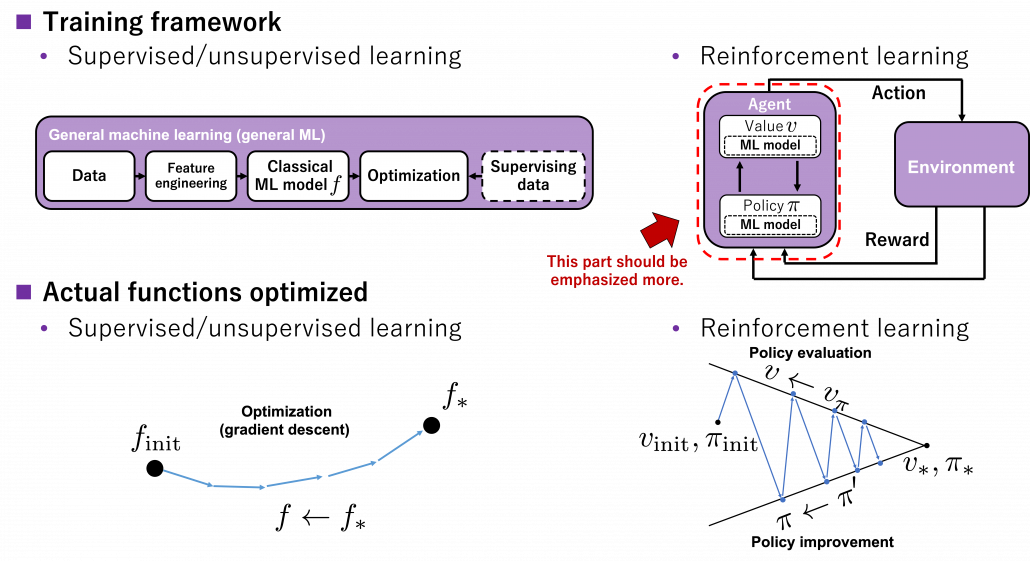
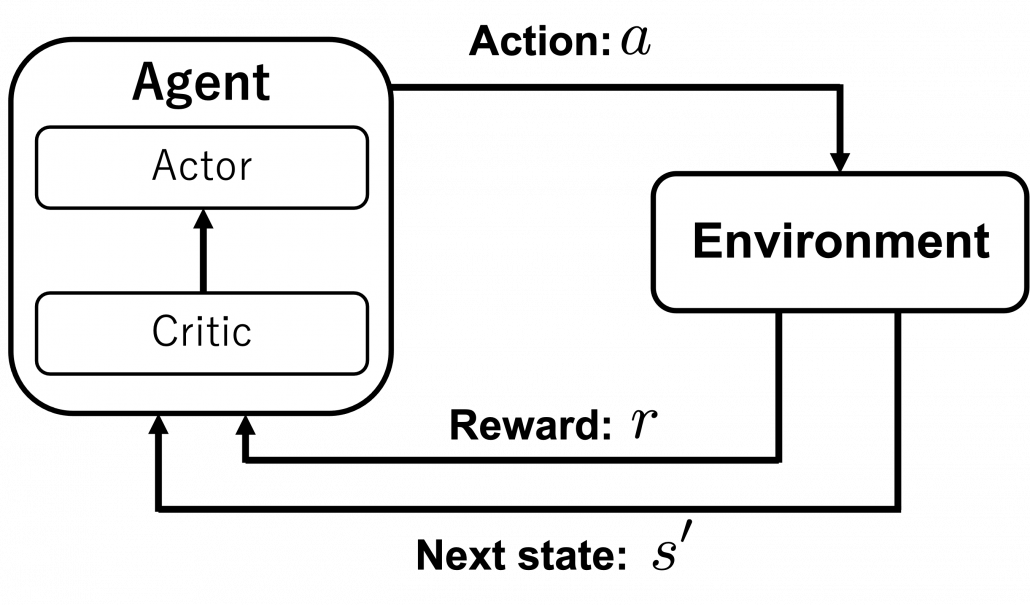
 , randomness of actions can be also learned by modeling policies with certain functions. This randomness of functions can be also modeled in actor-critic frameworks. That means, depending on a choice of an actor, such actor can learn randomness of actions, that is explorations.
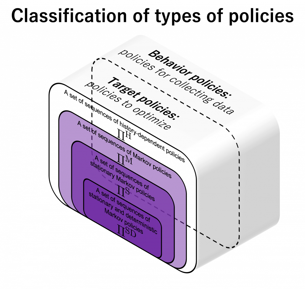
 , and gives out the next state
  and corresponding reward
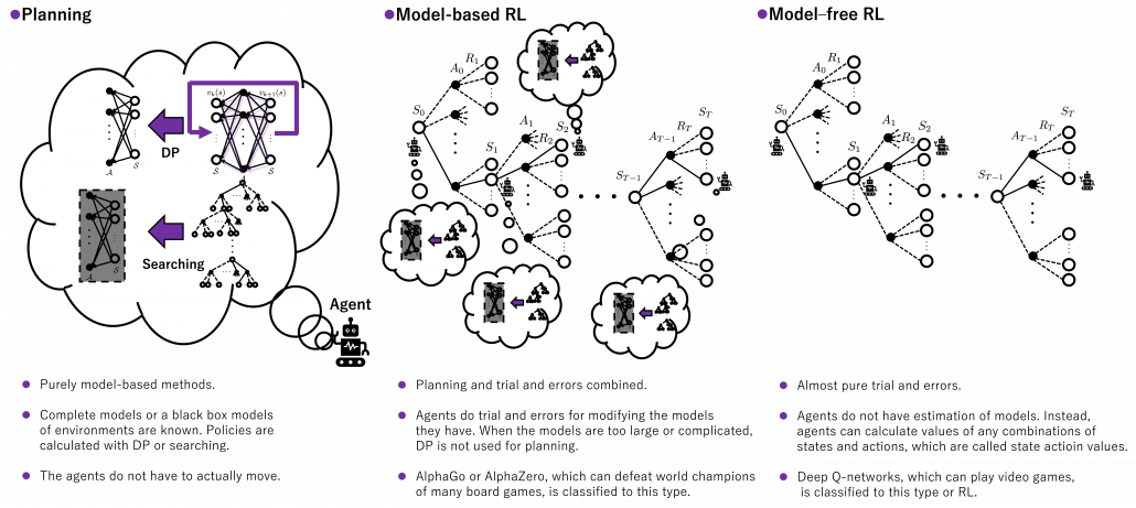
  , that is the black box is a sample model. In this case other planning methods with some searching algorithms are used, for example Monte Carlo tree search. Such search algorithms are designed to more efficiently and sparsely search states and actions of interest. Many of searching algorithms used in RL make uses of tree structures. Model-based approaches can be roughly classified into three types below based on size or complication of models.
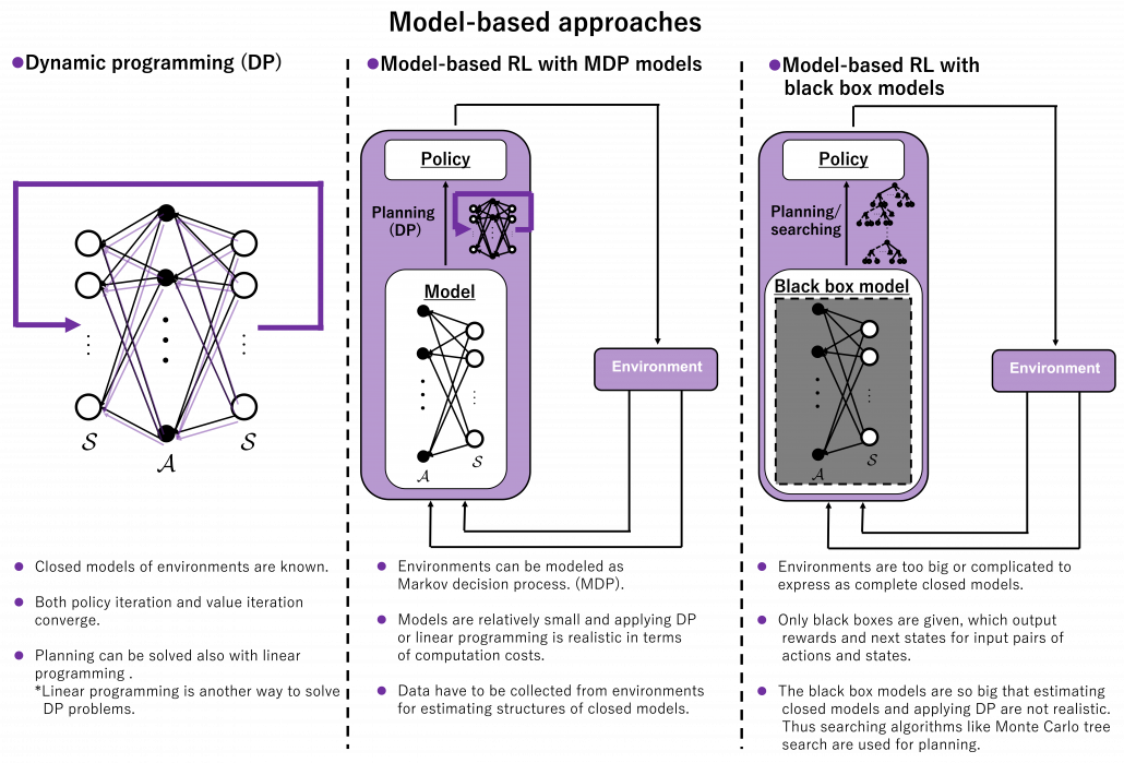
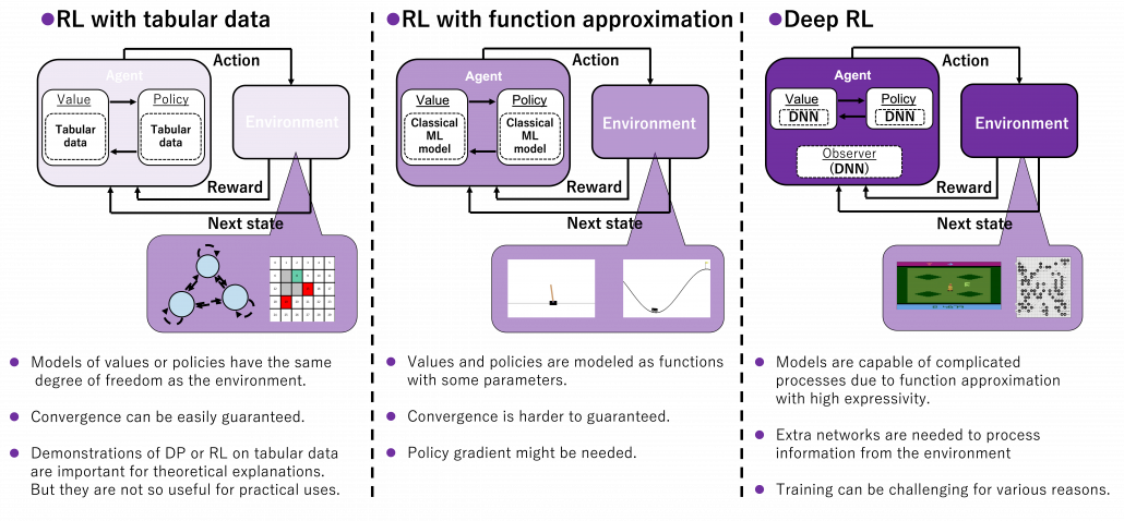 *And this spectrum is also a spectrum of computation costs or convergence. The left type could be easily implemented like programming assignments of schools since it in short needs only Excel sheets, and you would soon get results. The middle type would be more challenging, but that would not b computationally too expensive. But when it comes to the type at the right side, that is not something which should be done on your local computer. At least you need a GPU. You should expect some hours or days even for training RL agents to play 8 bit video games. That is of course due to cost of training deep neural networks (DNN), especially CNN. But another factors is potential inefficiency of RL. I hope I could explain those weak points of RL and remedies for them.
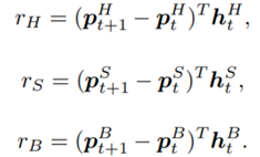
 , the total value
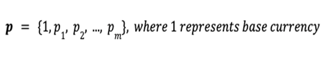
  of the portfolio is defined as the inner product of the price vector
  and the portfolio vector
  .
. at the terminal time step
  .
.
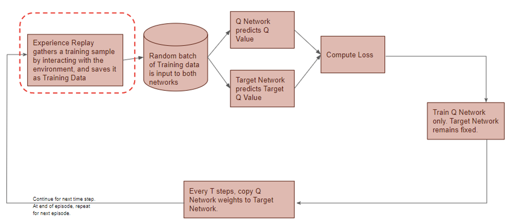
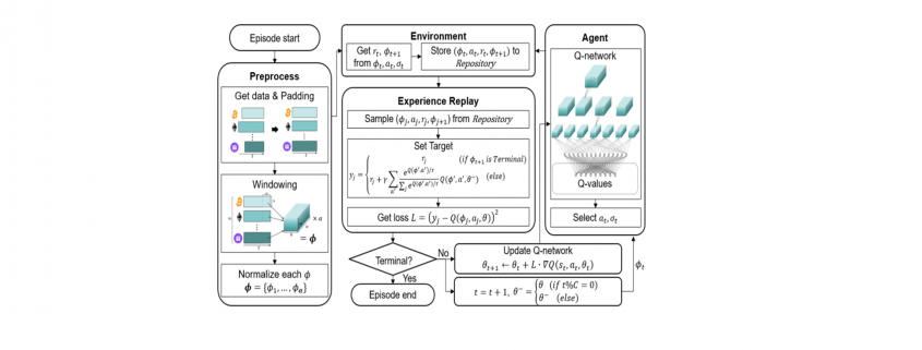
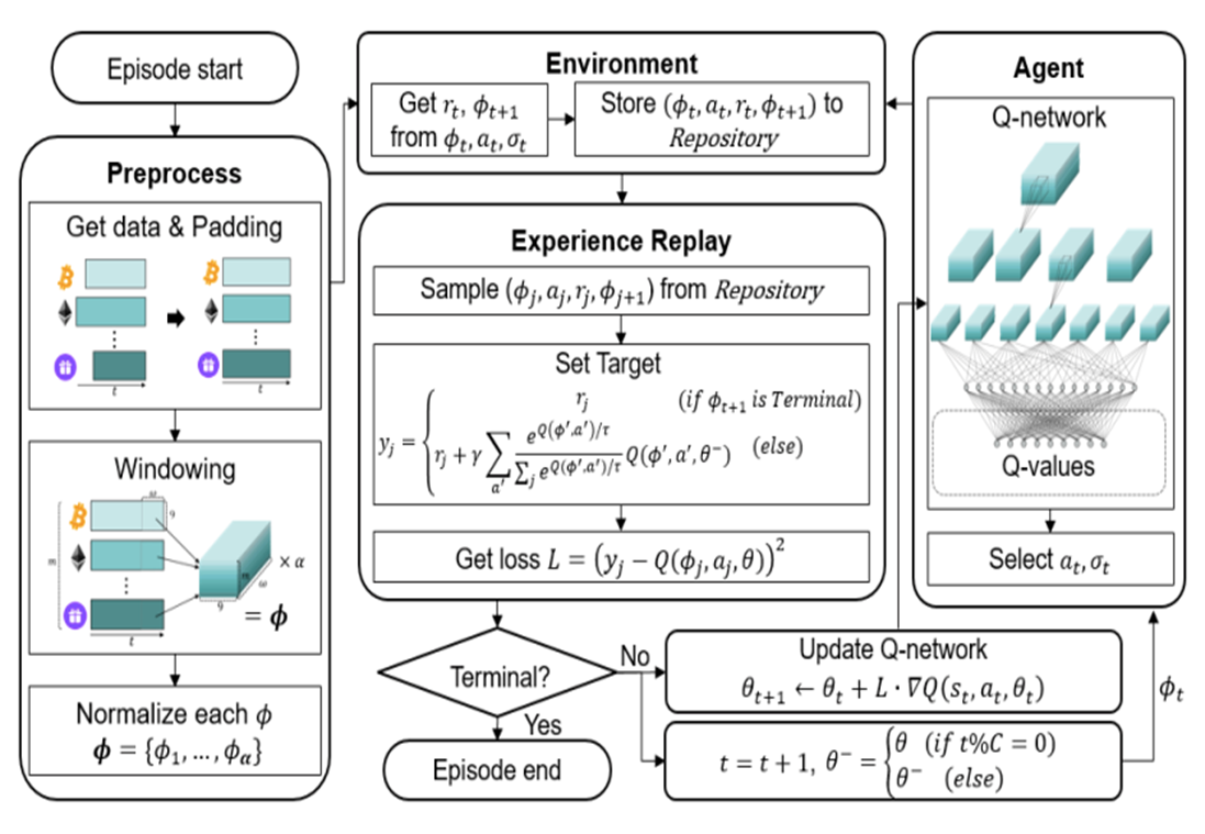
 ) is stored in the repository as a sample of training data.
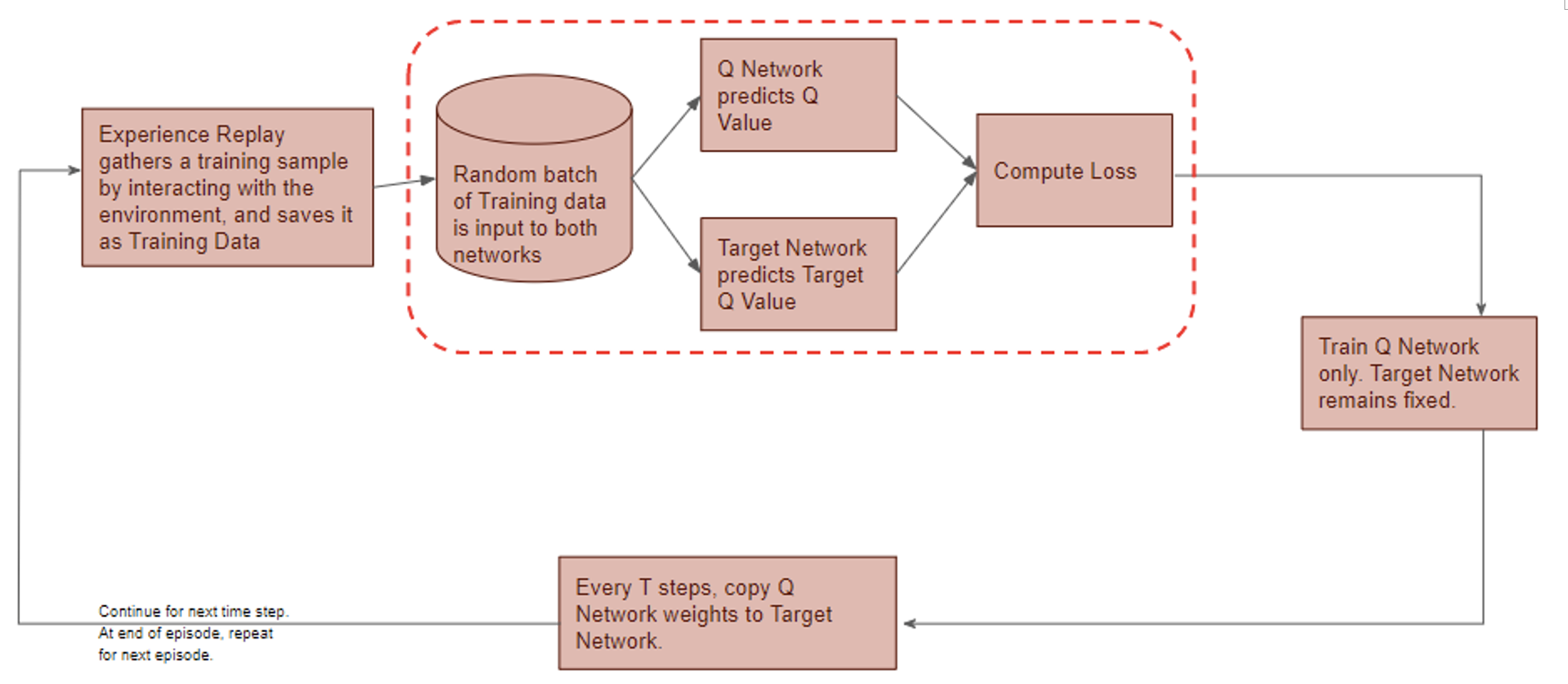
 is defined as the softmax value for the q-value of each action (ie. i-th asset at
  , then i-th asset is bought using 50% of base currency).
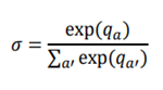
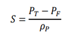
 is the return of a risk-free asset, which is set to 0 here.
 are initialized to 0, while the policy π(s) is uniformly distributed among all actions. Afterwards, everything is updated through interacting with the stock market environment. By the Bellman Equation,
  is the expectation of the sum of direct reward
  and the future reqard
  at the next state discounted by a factor γ, resulting in the state-action value function:
![[b_t, p_t, h_t, M_t, R_t, C_t, X_t]](https://data-science-blog.com/en/wp-content/ql-cache/quicklatex.com-0fbdf800e4e901e62bc4396f3815d15f_l3.png "Rendered by QuickLaTeX.com") storing information about
storing information about : Portfolio balance
 : Shares owned of each stock
 : Moving Average Convergence Divergence
 : Commodity Channel Index
 : Average Directional Index
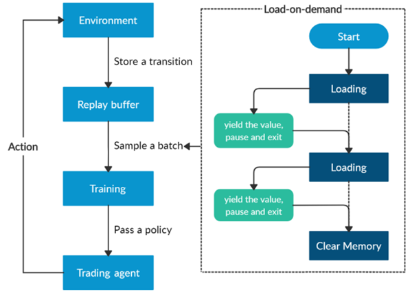
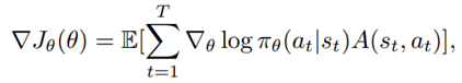
 is the policy network, and
  is the advantage function to reduce the high variance of it:
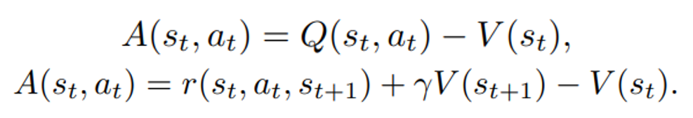
 is the value function of state

 is known, and
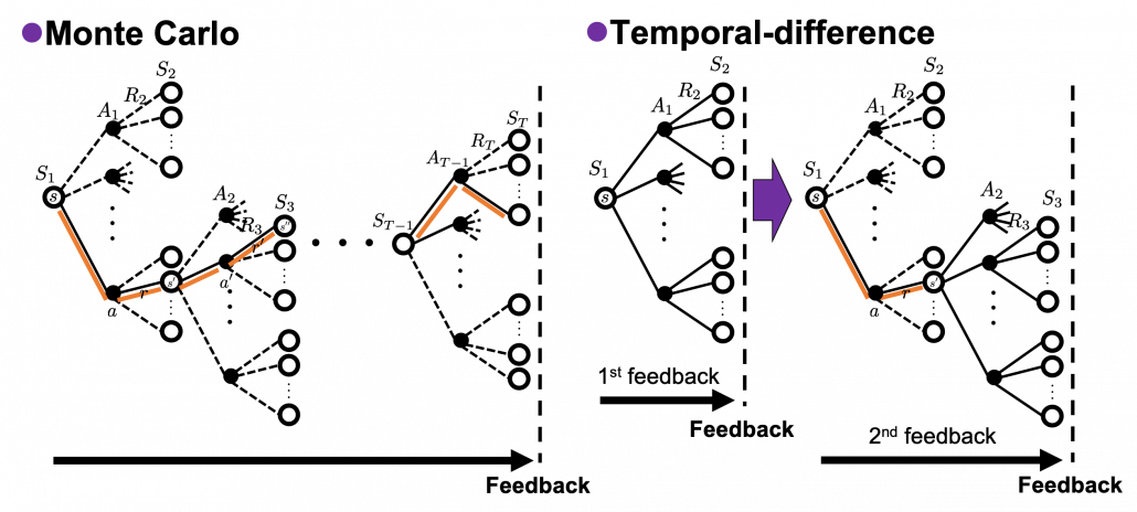
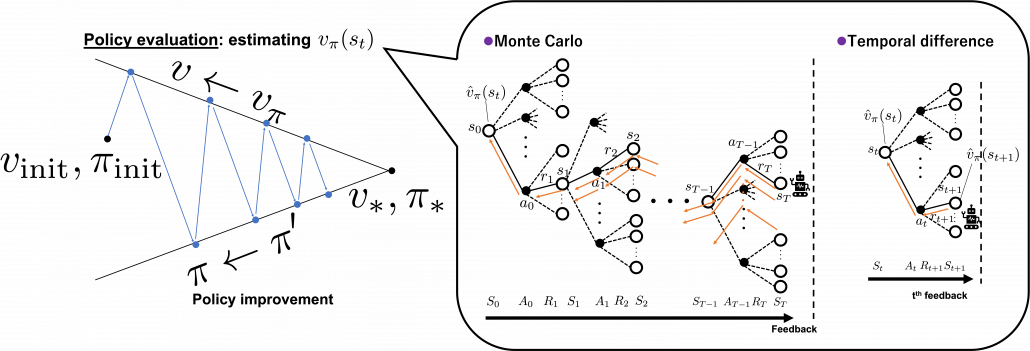
 ![v_{\pi} (s)\doteq \mathbb{E}_{\pi} [ G_t | S_t =s ] =\mathbb{E}_{\pi} [ R_{t+1} + \gamma R_{t+2} + \gamma ^2 R_{t+3} + \cdots + \gamma ^{T-t -1} R_{T} |S_t =s]](https://data-science-blog.com/en/wp-content/ql-cache/quicklatex.com-10b9dc282a7d98ce7ecaf0316096f9c9_l3.png "Rendered by QuickLaTeX.com")
 like
like  . But the number
 ![v_{\pi} (s)= \mathbb{E}_{\pi} [ R_{t+1} + \gamma v_{\pi}(S_{t+1}) | S_t =s ]](https://data-science-blog.com/en/wp-content/ql-cache/quicklatex.com-349331e8707784287bb3fd227c4f03af_l3.png "Rendered by QuickLaTeX.com")
 at the left side,
 ![v_{k+1} (s)\doteq \mathbb{E}_{\pi} [ R_{t+1} + \gamma v_{k}(S_{t+1}) | S_t =s ]](https://data-science-blog.com/en/wp-content/ql-cache/quicklatex.com-ba20177dbed44812a6f2ce98154e2c2e_l3.png "Rendered by QuickLaTeX.com")
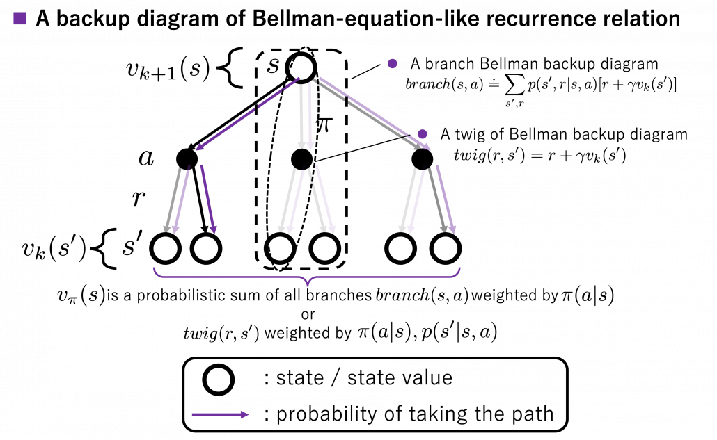
 , namely a probabilistic sum of future rewards is defined as follows.
![v_{k+1} (s) = \mathbb{E}_{\pi} [R_{t+1} + \gamma v_k (S_{t+1}) | S_t = s] \doteq \sum_a {\pi(a|s)} \sum_{s', r} {p(s', r|s, a)[r + \gamma v_k(s')]}](https://data-science-blog.com/en/wp-content/ql-cache/quicklatex.com-1a1aa71a4846a76bd8220751fa988103_l3.png "Rendered by QuickLaTeX.com")
 are probabilities of transitions. Policies are probabilities of taking an action
  weighted by
  weighted by
  . “Branches” and “twigs” are terms which I coined.
 is calculated like in the figure below, using values of
  . As I explained earlier, the value of the state
  is a sum of
  . And I showed the weight as strength of purple color of the arrows.
  are corresponding rewards of each transition. And importantly, the Bellman-equation-like operation, whish is a part of DP, is conducted inside the agent. The agent does not have to actually move, and that is what planning is all about.
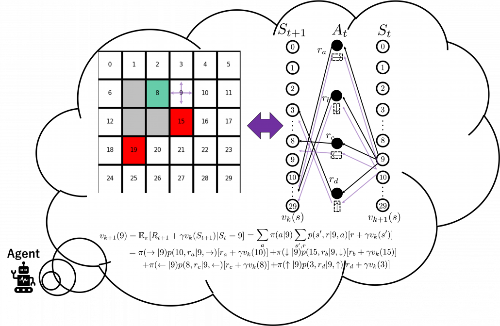
 to
to  . I tried to show the idea that values
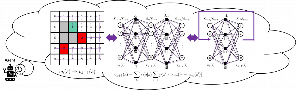
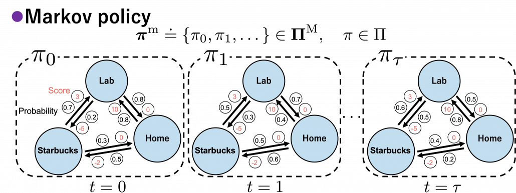
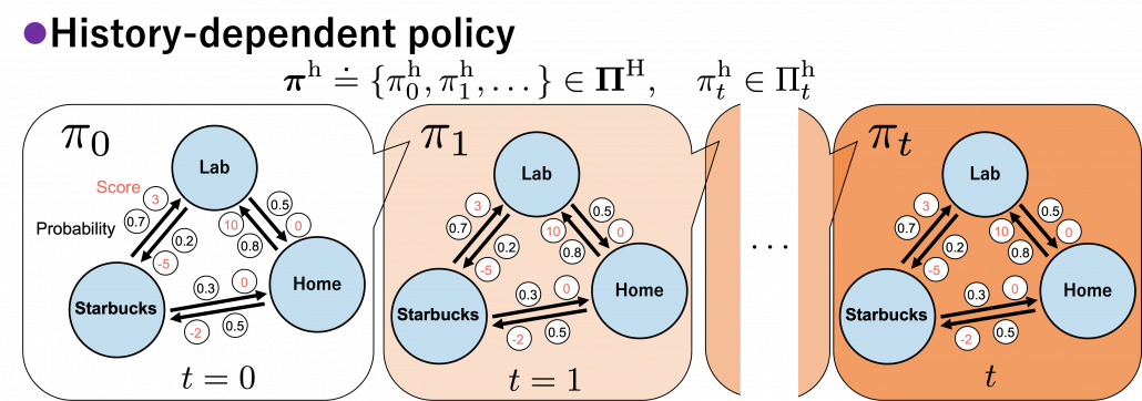
 in the figure below are of interest when you learn RL as a beginner. I am going to explain what each set of policies means one by one.
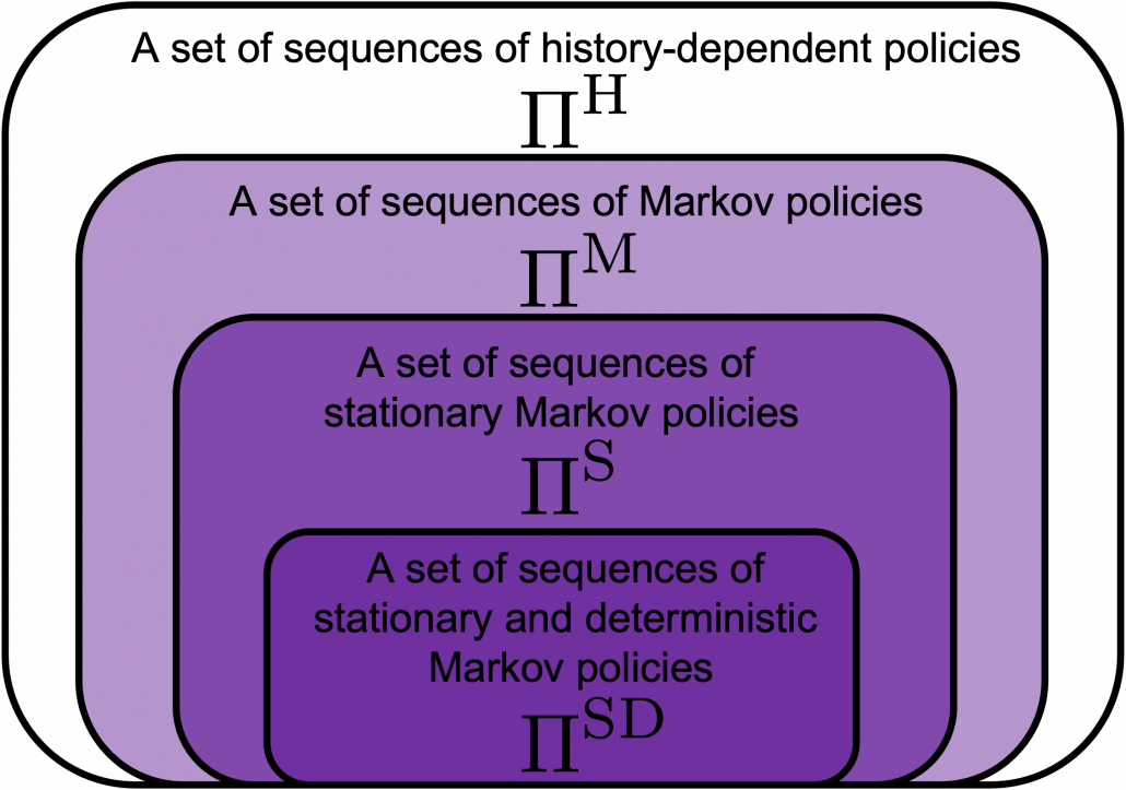
 , which mean probabilistic Markov policies. Remember that in the first article I explained Markov decision processes can be described like diagrams of daily routines. For example, the diagrams below are my daily routines. The indexes
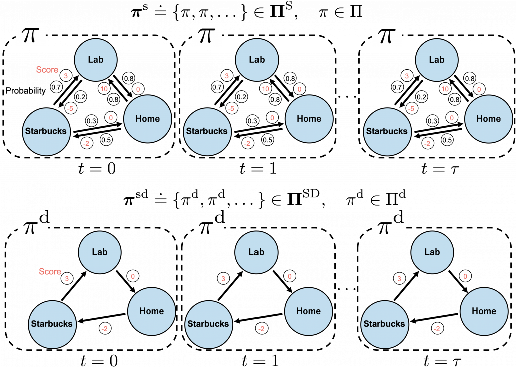
![\Pi \doteq \biggl\{ \pi : \mathcal{A}\times\mathcal{S} \rightarrow [0, 1]: \sum_{a \in \mathcal{A}}{\pi (a|s) =1, \forall s \in \mathcal{S} } \biggr\}](https://data-science-blog.com/en/wp-content/ql-cache/quicklatex.com-9a217cc6d5cfd59e564fd2132620f89f_l3.png "Rendered by QuickLaTeX.com")
 maps any combinations of an action
  and a state
  to a probability. The diagram above means you choose a policy
  , and you use the policy every time step
  . And a set of such stationary Markov policy sequences is denoted as
  .
. are called deterministic policies.
 .
.
 . However as I said, only
  in the context of DP or RL are defined as follows.

 is a random variable, and
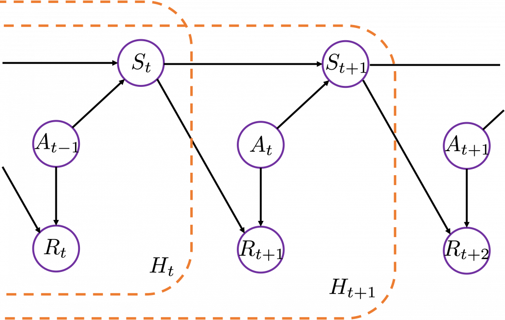
![\Pi _{t}^{\text{h}} \doteq \biggl\{ \pi _{t}^{h} : \mathcal{A}\times\mathcal{H}_t \rightarrow [0, 1]: \sum_{a \in \mathcal{A}}{\pi_{t}^{\text{h}} (a|h_{t}) =1 } \biggr\}](https://data-science-blog.com/en/wp-content/ql-cache/quicklatex.com-6414a4a7c3e4041e14077fce7a8c3fa1_l3.png "Rendered by QuickLaTeX.com")
 .
. or
or  is defined as the maximum value functions for all states
  .
.

 . That means, in the example graphical models I displayed, you just have to deterministically go back and forth between the lab and the home in order to maximize value function, never stopping by at a Starbucks. Also you do not have to change your plans depending on days.
 is defined. But to make things easier for now, let me skip ore precise formulations. Value functions are defined as expectations of rewards with respect to a single policy or a sequence of policies. You have only to keep it in mind that
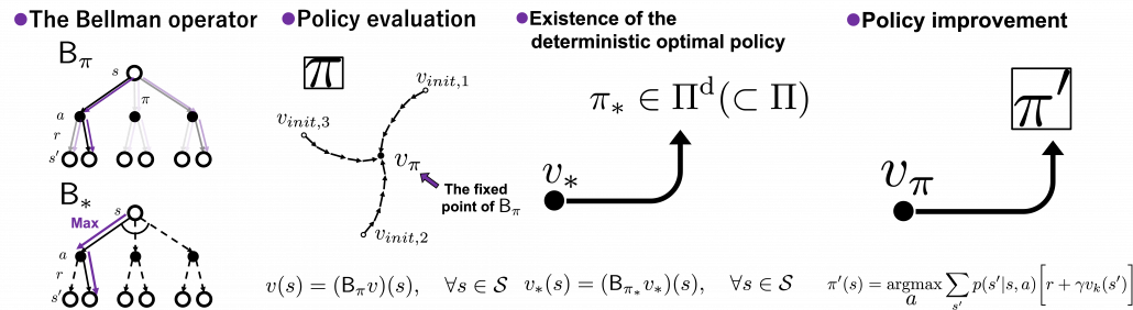
 or
or  .
. , which is deterministic. And it is an optimal policy if and only if it satisfies the Bellman expectation equation
  , with the optimal value function
  .
. , or rather an application of a Bellman expectation operator on any state functions
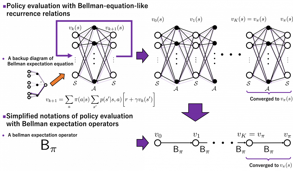
  is defined as below.
![(\mathsf{B}_{\pi} (v))(s) \doteq \sum_{a}{\pi (a|s)} \sum_{s'}{p(s'| s, a) \biggl[r + \gamma v (s') \biggr]}, \quad \forall s \in \mathcal{S}](https://data-science-blog.com/en/wp-content/ql-cache/quicklatex.com-35022b46d30c7f99c53089770a9dea7e_l3.png "Rendered by QuickLaTeX.com")
 . In the last article I explained that when
  is an arbitrarily initialized value function, a sequence of value functions
  converge to
 ![v_{k+1} = \sum_{a}{\pi (a|s)} \sum_{s'}{p(s'| s, a) \biggl[r + \gamma v_{k} (s') \biggr]}](https://data-science-blog.com/en/wp-content/ql-cache/quicklatex.com-792e43affeeb5f73e731a3bbd6469f93_l3.png "Rendered by QuickLaTeX.com")

 is obtained by applying
 times in total. Such operation is denoted as follows.
 converges to
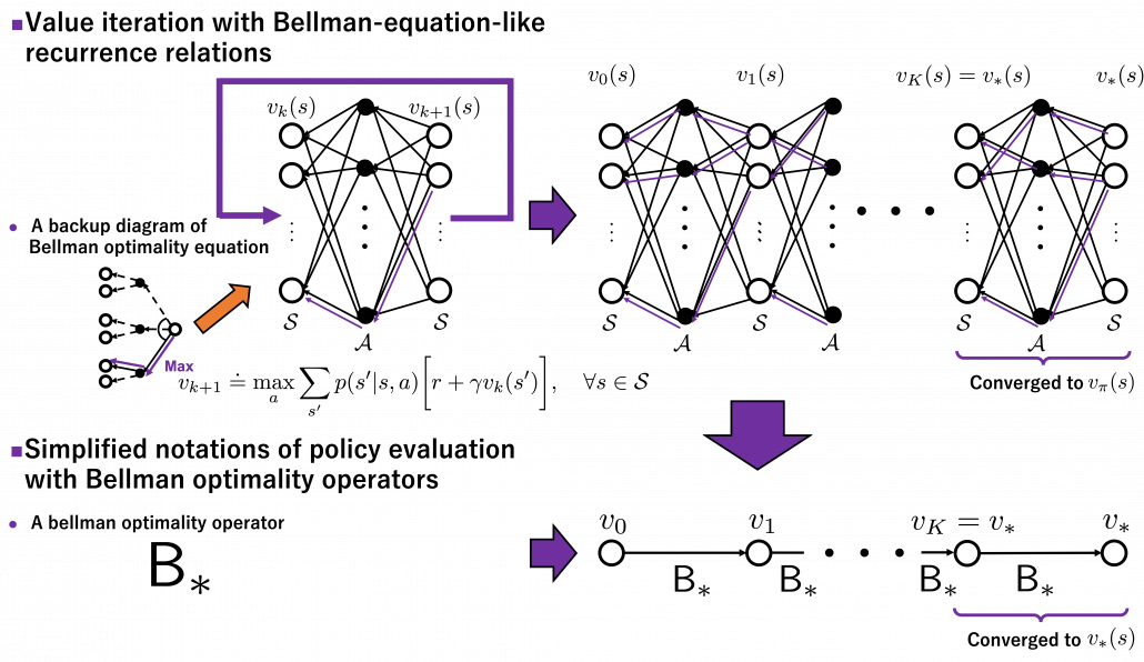
 is defined as follows.
![(\mathsf{B}_{\ast} v)(s) \doteq \max_{a} \sum_{s'}{p(s' | s, a) \biggl[r + \gamma v(s') \biggr]}, \quad \forall s \in \mathcal{S}](https://data-science-blog.com/en/wp-content/ql-cache/quicklatex.com-1c6fc7233a418b4abdfbde6886da4b58_l3.png "Rendered by QuickLaTeX.com")
 . With a Bellman optimality operator, you can get a recurrence relation
  . Multiple applications of Bellman optimality operators can be written down as below.
 converges to the optimal value function
 . If you apply Bellman operators of the policies one by one in an order of
  on a state function
  , the resulting state function is calculated as below.
 , we can also discuss convergence of
  , but that is just confusing. Please let me know if you are interested.
![v(s) = \sum_{a}{\pi (a|s)} \sum_{s'}{p(s'| s, a) \biggl[r + \gamma v (s') \biggr]}](https://data-science-blog.com/en/wp-content/ql-cache/quicklatex.com-d96ea8fd9bc433436f0c1636288df540_l3.png "Rendered by QuickLaTeX.com")
 . But whichever the notation is, the equation holds when the value function
  .
. , and the
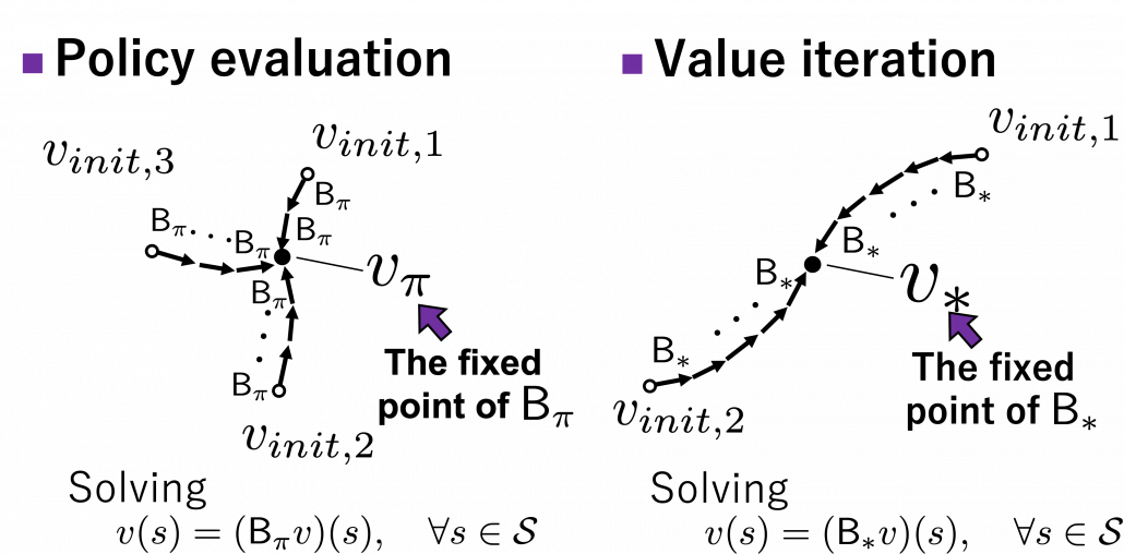
 . And also, you can judge whether a policy is optimal by a Bellman expectation equation below.
![\[v_{\ast}(s) = (\mathsf{B}_{\pi^{\ast} } v_{\ast})(s), \quad \forall s \in \mathcal{S} \]](https://data-science-blog.com/en/wp-content/ql-cache/quicklatex.com-c1a7be583f553c908c51f71b23ea4cff_l3.png "Rendered by QuickLaTeX.com")
![\[\pi^{\text{d}}_{\ast}(s) = \argmax_{a\in \matchal{A}} \sum_{s'}{p(s' | s, a) \biggl[r + \gamma v_{\ast}(s') \biggr]}, \quad \forall s \in \mathcal{S}\]](https://data-science-blog.com/en/wp-content/ql-cache/quicklatex.com-df3b441c33bb9e154ed039a5431676f9_l3.png "Rendered by QuickLaTeX.com")
 . After some calculations,
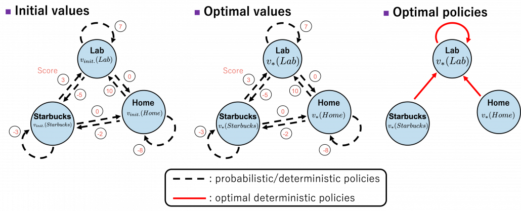
![b(s, a)\doteq\sum_{s'}{p(s' | s, a) \biggl[r + \gamma v_{\ast}(s') \biggr]} = r + \gamma \sum_{s'}{p(s' | s, a) v_{\ast}(s') }](https://data-science-blog.com/en/wp-content/ql-cache/quicklatex.com-cb95afc26ed333c0bc782b865d2595f1_l3.png "Rendered by QuickLaTeX.com") . Let me call the part
. Let me call the part  ” a value of a branch,” and finding the optimal deterministic policy is equal to choosing the maximum branch for all
  and all the all the states
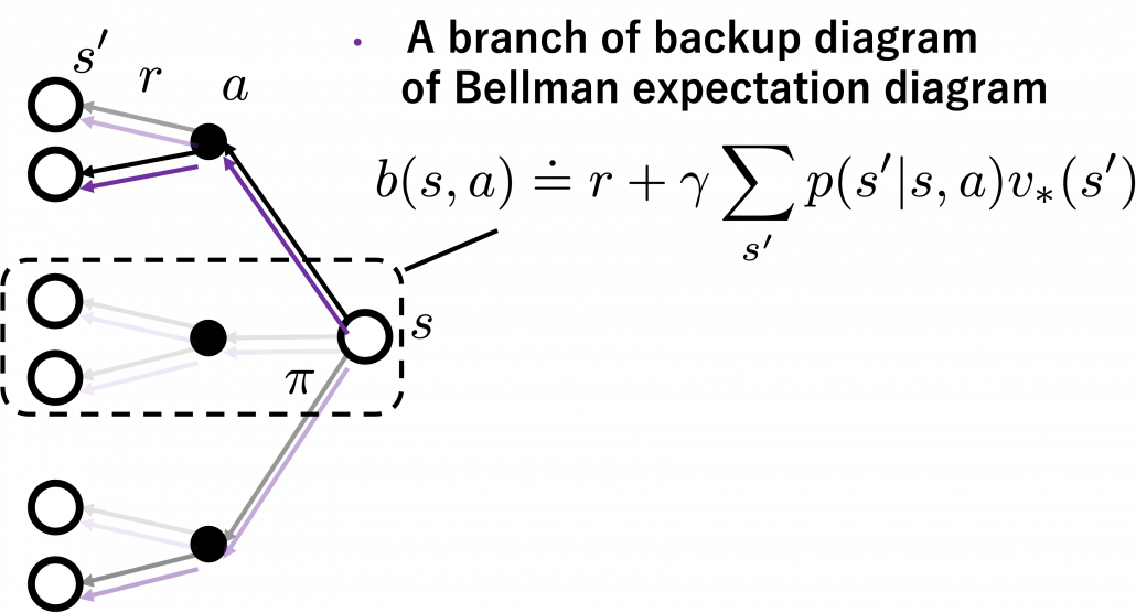
 , and after some iterations they converged to the optimal values. The numbers in each node are values of the sates. And the numbers next to each edge are corresponding values of branches
  . After you get the optimal value, if you choose the direction with the maximum branch at each state, you get the optimal deterministic policy. And that means “Just go to the lab, not Starbucks.”
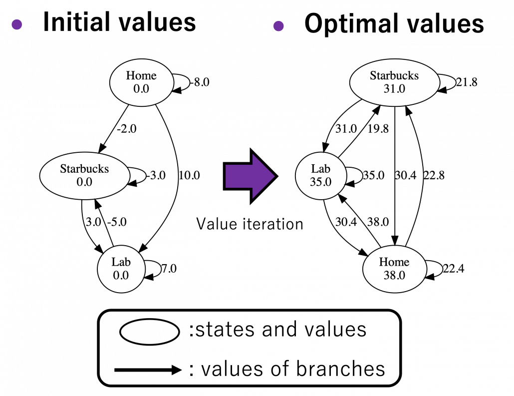
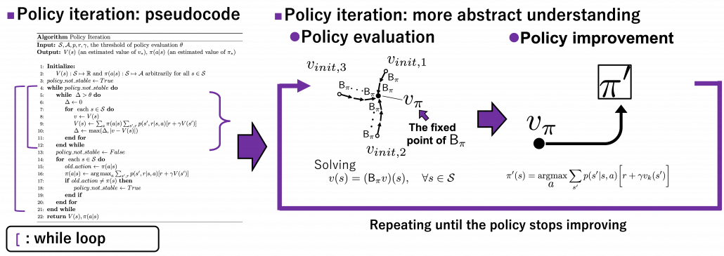
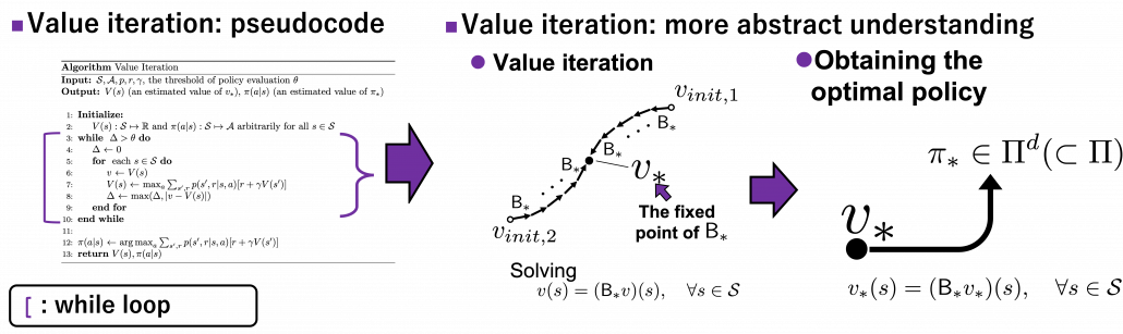
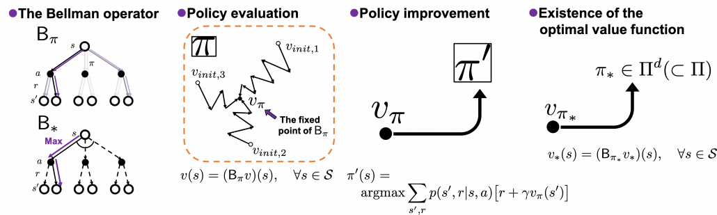
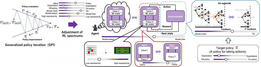
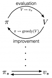 According to a famous Japanese textbook on RL named “Machine Learning Professional Series: Reinforcement Learning,” most study materials on RL lack explanations on mathematical foundations of RL, including the book by Sutton and Barto. That is why many people who have studied machine learning often find it hard to get RL formulations at the beginning. The book also points out that you need to refer to other bulky books on Markov decision process or dynamic programming to really understand the core ideas behind algorithms introduced in RL textbooks. And I got an impression most of study materials on RL get away with the important ideas on DP with only introducing value iteration and policy iteration algorithms. But my opinion is we should pay more attention on policy iteration. And actually important RL algorithms like Q learning, SARSA, or actor critic methods show some analogies to policy iteration. Also the book by Sutton and Barto also briefly mentions “Almost all reinforcement learning methods are well described as GPI (generalized policy iteration). That is, all have identifiable policies and value functions, with the policy always being improved with respect to the value function and the value function always being driven toward the value function for the policy, as suggested by the diagram to the right side.“
 , you need to calculate a value functions
 or
or  . But I would like you take it easy while reading my articles. I will repeatedly mentions differences of notations when that matters.
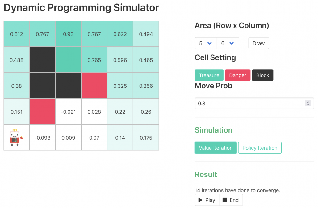

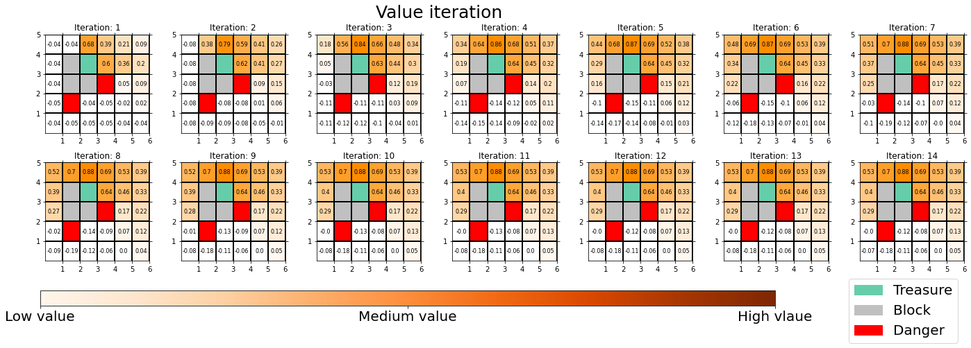
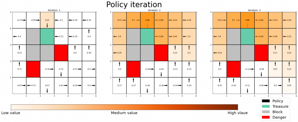
 grid map which I visualized above. In this case each cell is numbered from
  as the figure below. But the cell 7, 13, 14 are removed from the map. In this case
  , and
, and  . When you pass
  , you get a reward
  , and when you pass the states
  or
or  , you get a reward
  . Also, the agent is encouraged to reach the goal as soon as possible, thus the agent gets a regular reward of
  every time step.
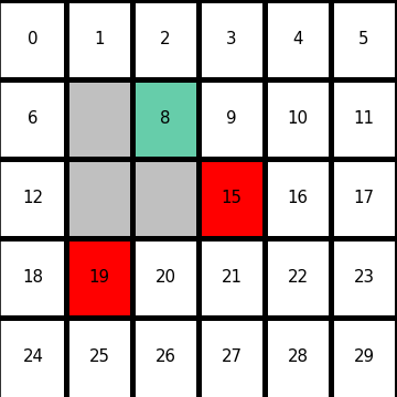

 needs to be considered. And this is the value of the state. Thus the value of a state
 ![\mathbb{E}_{\pi}\bigl[R_{t+1} + R_{t+2} + R_{t+3} + \cdots + R_T | S_t = s \bigr]](https://data-science-blog.com/en/wp-content/ql-cache/quicklatex.com-1446ab2bd566ff9ae22a26979bc864a2_l3.png "Rendered by QuickLaTeX.com")
 , it can take numerous patterns of actions. For example (a)
  , (b)
, (b)  , (c)
, (c)  . The rewards after each behavior is calculated as follows.
 in total. The probability of taking a course of a) is


 is
is  . The probability of taking the action can be calculated in the same way as
 .
.![\mathbb{E}_{\pi}\bigl[R_{t+1} + R_{t+2} + R_{t+3} + \cdots + R_T | S_t = s \bigr] = r_a \cdot p_a + r_b \cdot p_b](https://data-science-blog.com/en/wp-content/ql-cache/quicklatex.com-9af1a6e1d05f0e084ca3df7b2cab9ef9_l3.png "Rendered by QuickLaTeX.com")
 ,and it is virtually equal to considering all the possible future cases.A very important formula named the Bellman equation effectively formulate that.
![\gamma \in (0, 1]](https://data-science-blog.com/en/wp-content/ql-cache/quicklatex.com-914da56af30aaafcc35b558976e8fdca_l3.png "Rendered by QuickLaTeX.com") is a discount rate. (1)As the first point above, the discounted return can be calculated recursively as follows:
is a discount rate. (1)As the first point above, the discounted return can be calculated recursively as follows: 

 . You can postpone calculation of future rewards corresponding to
  this way. This might sound obvious, but this small trick is crucial for defining defining value functions or making update rules of them. (2)The second point might be confusing to some people, but it is the most important in this section. We took a look at a very simplified case of calculating the expectation in the last section, but let’s see how a value function
 ![v_{\pi}(s) \doteq \mathbb{E}_{\pi}\bigl[G_t | S_t = s \bigr]](https://data-science-blog.com/en/wp-content/ql-cache/quicklatex.com-4a07b7408b4cebfe6e2558ca8d1573cf_l3.png "Rendered by QuickLaTeX.com")
![v_{\pi} (s)= \sum_{a}{\pi(a|s) \sum_{s', r}{p(s', r|s, a)\bigl[r + \gamma v_{\pi}(s')\bigr]}}](https://data-science-blog.com/en/wp-content/ql-cache/quicklatex.com-9b05fc8f5122733b29e251f8000f7bf2_l3.png "Rendered by QuickLaTeX.com")
![\sum_{s', r, a}{\pi(a|s) p(s', r|s, a)\bigl[r + \gamma v_{\pi}(s')\bigr]}](https://data-science-blog.com/en/wp-content/ql-cache/quicklatex.com-c9afc3114f14adcf06a184c6656f404b_l3.png "Rendered by QuickLaTeX.com") . It can be comprehended this way: in Bellman equation you calculate a probabilistic sum of
. It can be comprehended this way: in Bellman equation you calculate a probabilistic sum of  , considering all the possible actions of the agent in the time step.
  . Hence the right side of Bellman equation above means the sum of
 ![\pi(a|s) p(s', r|s, a)\bigl[r + \gamma v_{\pi}(s')\bigr]](https://data-science-blog.com/en/wp-content/ql-cache/quicklatex.com-c68792d33ebf817bf92b2c3122432011_l3.png "Rendered by QuickLaTeX.com") , over all possible combinations of
, over all possible combinations of  . In order to calculate the expectation, you have to consider all the combinations of
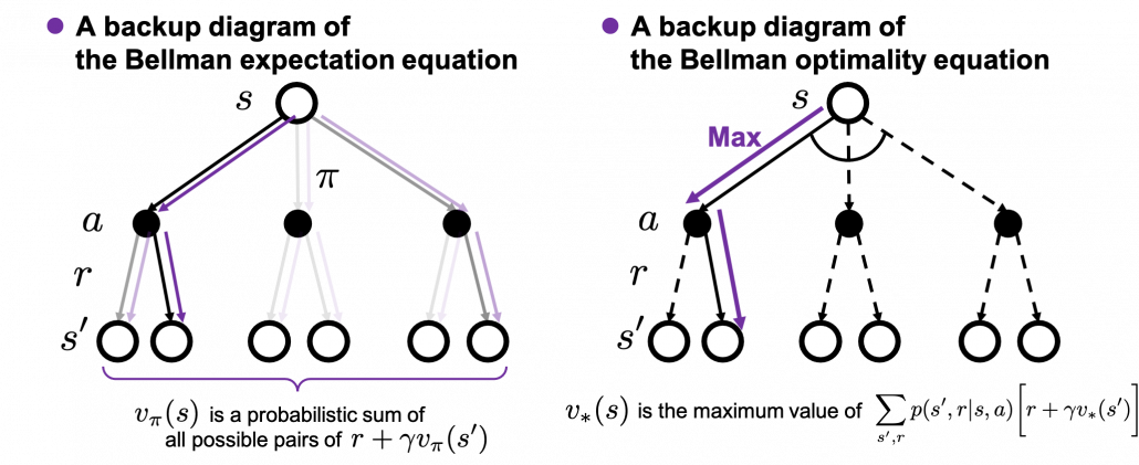
![v_{\ast}(s) \doteq \max_{a} \sum_{s', r}{p(s', r|s, a)\bigl[r + \gamma v_{\ast}(s')\bigr]}](https://data-science-blog.com/en/wp-content/ql-cache/quicklatex.com-86f7734f497416e3b1922ee15d1688dc_l3.png "Rendered by QuickLaTeX.com")
 are known, a major way of calculating
  converges to
 ![v_{k+1}(s) =\sum_{a}{\pi(a|s)\sum_{s', r}{p(s', r | s, a) [r + \gamma v_k (s')]}}](https://data-science-blog.com/en/wp-content/ql-cache/quicklatex.com-0d6a73bc17d541f77b43a10e128462ce_l3.png "Rendered by QuickLaTeX.com") .
.![v_{\pi}(s) =\sum_{a}{\pi(a|s)\sum_{s', r}{p(s', r | s, a) [r + \gamma v_{\pi} (s')]}}](https://data-science-blog.com/en/wp-content/ql-cache/quicklatex.com-afdb0cd8be05e7e79fc3306f8ebc3732_l3.png "Rendered by QuickLaTeX.com") .
. to the converged state at
  . But you have to be careful abut the directions of the arrows in purple. If you correspond the backup diagrams of the Bellman equation with the graphs below, the purple arrows point to the reverse side to the direction where the graphs extend. This process of converging an arbitrarily initialized
  to
to 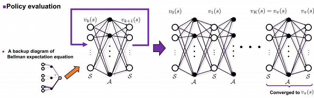
 are a set of states and actions respectively. Thus
  , the size of
 ![v_{k+1}(s) =\max_a\sum_{s', r}{p(s', r | s, a) [r + \gamma v_k (s')]}](https://data-science-blog.com/en/wp-content/ql-cache/quicklatex.com-798ecf9bb29b6fcdecb3282f759d07d2_l3.png "Rendered by QuickLaTeX.com")
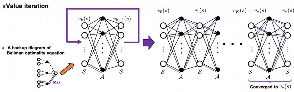
![\pi(a|s) \gets\text{argmax}_a {r + \sum_{s', r}{p(s', r|s, a)[r + \gamma V(s')]}}, \quad \forall s\in \mathcal{S}](https://data-science-blog.com/en/wp-content/ql-cache/quicklatex.com-5f4b9305832f16e171d2d5428f5251d8_l3.png "Rendered by QuickLaTeX.com")
![r + \sum_{s', r}{p(s', r|s, a)[r + \gamma V(s')]}](https://data-science-blog.com/en/wp-content/ql-cache/quicklatex.com-3cb4dfa2cd76474740b41aecacce9d84_l3.png "Rendered by QuickLaTeX.com") is maximized. And when the policy
is maximized. And when the policy 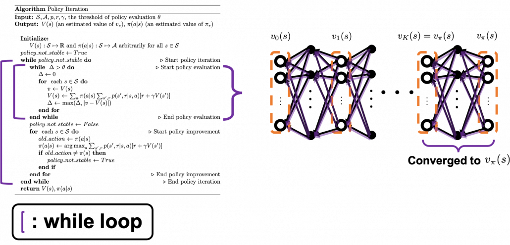
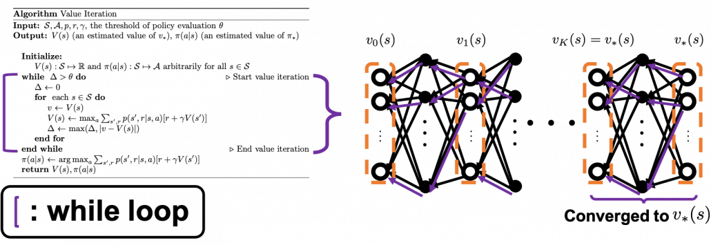
 . And corresponding small letters are realized values of the random variables. For example
  . (*Please do not think too much about the number of
  s on the small letters.)
 . This means the probability of
  are sampled given that
  is sampled.
 means a probability of transition, but I am using
  shows the probability that, given an agent being in state
  , and receive reward
  . Thus importantly,
 are discrete random variables, a conditional expectation of
  given
given  is calculated as follows:
 ![\mathbb{E}[X|Y=y] = \sum_{x}{p(x|Y=y)}](https://data-science-blog.com/en/wp-content/ql-cache/quicklatex.com-5bee0d95ebfa141ff0bc520462f4cfa9_l3.png "Rendered by QuickLaTeX.com") .
. and linearity of an expectation, the following equations hold.
![v_{\pi}(s) = \mathbb{E} [G_t | S_t =s] = \mathbb{E} [R_{t+1} + \gamma G_{t+1} | S_t =s]](https://data-science-blog.com/en/wp-content/ql-cache/quicklatex.com-fbb4801687a26cb911e5675ac25002bd_l3.png "Rendered by QuickLaTeX.com")
![=\mathbb{E} [R_{t+1} | S_t =s] + \gamma \mathbb{E} [G_{t+1} | S_t =s]](https://data-science-blog.com/en/wp-content/ql-cache/quicklatex.com-f485080bf287c6c9156187adc49b1b4c_l3.png "Rendered by QuickLaTeX.com")
![\mathbb{E} [R_{t+1} | S_t =s]](https://data-science-blog.com/en/wp-content/ql-cache/quicklatex.com-a585f119409ea2b556c68a0c1378a356_l3.png "Rendered by QuickLaTeX.com") and
and ![\mathbb{E} [G_{t+1} | S_t =s]](https://data-science-blog.com/en/wp-content/ql-cache/quicklatex.com-7f1e5cf67a9196db4f0aace79e81e322_l3.png "Rendered by QuickLaTeX.com") . As I have explained
. As I have explained  over all the combinations of
  . And according to one of the points above,
  . Thus the following equation holds.
![\mathbb{E} [R_{t+1} | S_t =s] = \sum_{s', a, r}{p(s', a, r|s)r} =](https://data-science-blog.com/en/wp-content/ql-cache/quicklatex.com-dd202255b6a36417c897509dc2b69655_l3.png "Rendered by QuickLaTeX.com")
 .
.![\mathbb{E} [G_{t+1} | S_t =s]](https://data-science-blog.com/en/wp-content/ql-cache/quicklatex.com-6bc115f9e71f2fc3a69465acf6a91464_l3.png "Rendered by QuickLaTeX.com")
![= \mathbb{E} [R_{t + 2} + \gamma R_{t + 3} + \gamma ^2 R_{t + 4} + \cdots | S_t =s]](https://data-science-blog.com/en/wp-content/ql-cache/quicklatex.com-48b09c6d0d7d67902de3191e66a38be2_l3.png "Rendered by QuickLaTeX.com")
![= \mathbb{E} [R_{t + 2} | S_t =s] + \gamma \mathbb{E} [R_{t + 2} | S_t =s] + \gamma ^2\mathbb{E} [ R_{t + 4} | S_t =s] +\cdots](https://data-science-blog.com/en/wp-content/ql-cache/quicklatex.com-5cdf22993b5055312df2e1f797fd3b26_l3.png "Rendered by QuickLaTeX.com") .
.![\mathbb{E} [R_{t + 2} | S_t =s]](https://data-science-blog.com/en/wp-content/ql-cache/quicklatex.com-469530b7d89bba0e743a0a3b1015ccd3_l3.png "Rendered by QuickLaTeX.com") . Also
. Also ![\mathbb{E} [R_{t + 3} | S_t =s]](https://data-science-blog.com/en/wp-content/ql-cache/quicklatex.com-2bb7f6a67696da895bb485861837f1d2_l3.png "Rendered by QuickLaTeX.com") is a sum of
is a sum of  over all the combinations of (s”, a’, r’, s’, a, r).
![\mathbb{E}_{\pi} [R_{t + 2} | S_t =s] =\sum_{s'', a', r', s', a, r}{p(s'', a', r', s', a, r|s)r'}](https://data-science-blog.com/en/wp-content/ql-cache/quicklatex.com-616b7769fe43ea42b46e5ca3f604ccee_l3.png "Rendered by QuickLaTeX.com")


 and the reward
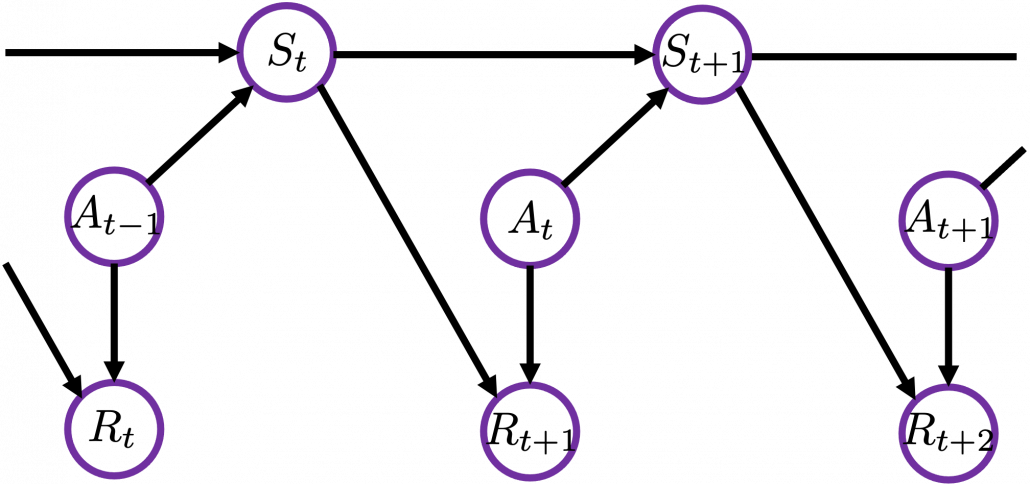
 , only
  . And again
  . Thus the following equations hold.
![\mathbb{E}_{\pi} [R_{t + 2} | S_t =s]=\sum_{ s', a, r}{p(s', a, r|s)} \sum_{s'', a', r'}{p(s'', a', r'| s', a, r', s)r'}](https://data-science-blog.com/en/wp-content/ql-cache/quicklatex.com-1e4e2cb83f6dd183dce4e2a51990bbc2_l3.png "Rendered by QuickLaTeX.com")

![= \sum_{ s', a, r}{p(s', r|a, s)\pi(a|s)} \mathbb{E}_{\pi} [R_{t+2} | s']](https://data-science-blog.com/en/wp-content/ql-cache/quicklatex.com-664e5538f363a0ef817dd5f48fbbae6a_l3.png "Rendered by QuickLaTeX.com") .
.![\mathbb{E}_{\pi} [R_{t + 3} | S_t =s]](https://data-science-blog.com/en/wp-content/ql-cache/quicklatex.com-64827bc08e99d614dc3838a85798c7d8_l3.png "Rendered by QuickLaTeX.com") can be calculated the same way.
can be calculated the same way.![\mathbb{E}_{\pi}[R_{t + 3} | S_t =s] =\sum_{s''', a'', r'', s'', a', r', s', a, r}{p(s''', a'', r'', s'', a', r', s', a, r|s)r''}](https://data-science-blog.com/en/wp-content/ql-cache/quicklatex.com-421e1a0b214d777abba77463656339f8_l3.png "Rendered by QuickLaTeX.com")


![=\sum_{ s', a, r}{ p(s', r | s, a)p(a|s)} \mathbb{E}_{\pi} [R_{t+3} | s']](https://data-science-blog.com/en/wp-content/ql-cache/quicklatex.com-6e0ec2657d6aca22c01de6f4b10a136a_l3.png "Rendered by QuickLaTeX.com") .
.![\mathbb{E}_{\pi} [R_{t + 4} | S_t =s]](https://data-science-blog.com/en/wp-content/ql-cache/quicklatex.com-5370726e4df48fa2beda19166dc02906_l3.png "Rendered by QuickLaTeX.com") ,
, ![\mathbb{E}_{\pi} [R_{t + 5} | S_t =s]\dots](https://data-science-blog.com/en/wp-content/ql-cache/quicklatex.com-c60185b7e16dd3c9d80041a6d63e4901_l3.png "Rendered by QuickLaTeX.com") . Thus
. Thus![v_{\pi}(s) =\mathbb{E} [R_{t+1} | S_t =s] + \gamma \mathbb{E} [G_{t+1} | S_t =s]](https://data-science-blog.com/en/wp-content/ql-cache/quicklatex.com-e78cd95d37820f82e6dce3d5c5943815_l3.png "Rendered by QuickLaTeX.com")
![+ \mathbb{E} [R_{t + 2} | S_t =s] + \gamma \mathbb{E} [R_{t + 3} | S_t =s] + \gamma ^2\mathbb{E} [ R_{t + 4} | S_t =s] +\cdots](https://data-science-blog.com/en/wp-content/ql-cache/quicklatex.com-9d5855daab70bbee7810386c6fc52bc1_l3.png "Rendered by QuickLaTeX.com")

![+\sum_{ s', a, r}{p(s', r|a, s)\pi(a|s)} \mathbb{E}_{\pi} [R_{t+2} |S_{t+1}= s']](https://data-science-blog.com/en/wp-content/ql-cache/quicklatex.com-028766cd22f5479faa5a4f1ea907da6b_l3.png "Rendered by QuickLaTeX.com")
![+\gamma \sum_{ s', a, r}{ p(s', r | s, a)p(a|s)} \mathbb{E}_{\pi} [R_{t+3} |S_{t+1} = s']](https://data-science-blog.com/en/wp-content/ql-cache/quicklatex.com-6679a24522d25f8e36d5caf2a7a8ce06_l3.png "Rendered by QuickLaTeX.com")
![+\gamma^2 \sum_{ s', a, r}{ p(s', r | s, a)p(a|s)} \mathbb{E}_{\pi} [ R_{t+4}|S_{t+1} = s'] + \cdots](https://data-science-blog.com/en/wp-content/ql-cache/quicklatex.com-cb1b0cd6d79e351b146b9b5766c7f5e2_l3.png "Rendered by QuickLaTeX.com")
![=\sum_{ s', a, r}{ p(s', r | s, a)p(a|s)} [r + \mathbb{E}_{\pi} [\gamma R_{t+2}+ \gamma R_{t+3}+\gamma^2R_{t+4} + \cdots |S_{t+1} = s'] ]](https://data-science-blog.com/en/wp-content/ql-cache/quicklatex.com-641a5ebcd67a76dc3f5367ee009e9b14_l3.png "Rendered by QuickLaTeX.com")
![=\sum_{ s', a, r}{ p(s', r | s, a)p(a|s)} [r + \mathbb{E}_{\pi} [G_{t+1} |S_{t+1} = s'] ]](https://data-science-blog.com/en/wp-content/ql-cache/quicklatex.com-133e0a40144cd6b8d9d24eb9c62541a3_l3.png "Rendered by QuickLaTeX.com")
![=\sum_{ s', a, r}{ p(s', r | s, a)p(a|s)} [r + v_{\pi}(s') ]](https://data-science-blog.com/en/wp-content/ql-cache/quicklatex.com-942d98bd0c9d7cc3ed2939137e05df53_l3.png "Rendered by QuickLaTeX.com")
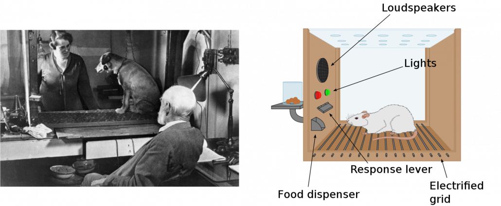

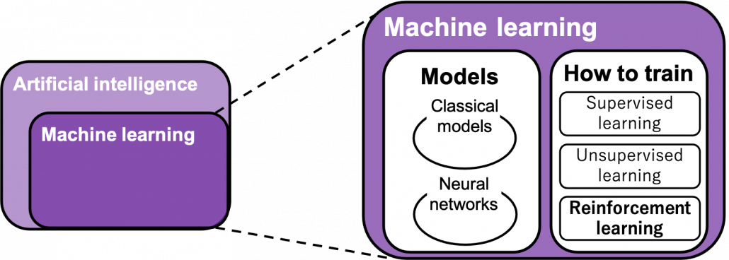 “Models” in the chart are often hyped as “AI” in media today. But AI is a more comprehensive field of trying to realize human-like intellectual behaviors with computers. And machine learning have been the most central sub-field of AI last decades. Around 2006 there was a breakthrough of deep learning. Due to the breakthrough machine learning gained much better performance with deep learning models. I would say people have been calling popular “models” in each time “AI.” And importantly, RL is one field of training models, besides supervised learning and unsupervised learning, rather than a field of designing “AI” models. Some people say supervised learning or unsupervised learning are more preferable than RL because currently these trainings are more likely to be more successful in wide range of fields than RL. And usually the more data you have the more likely supervised or unsupervised learning are.
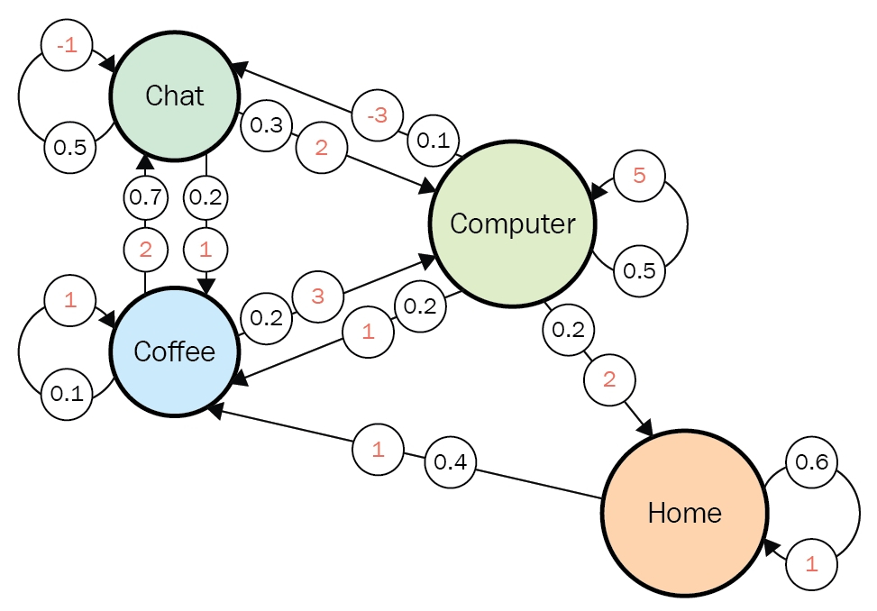
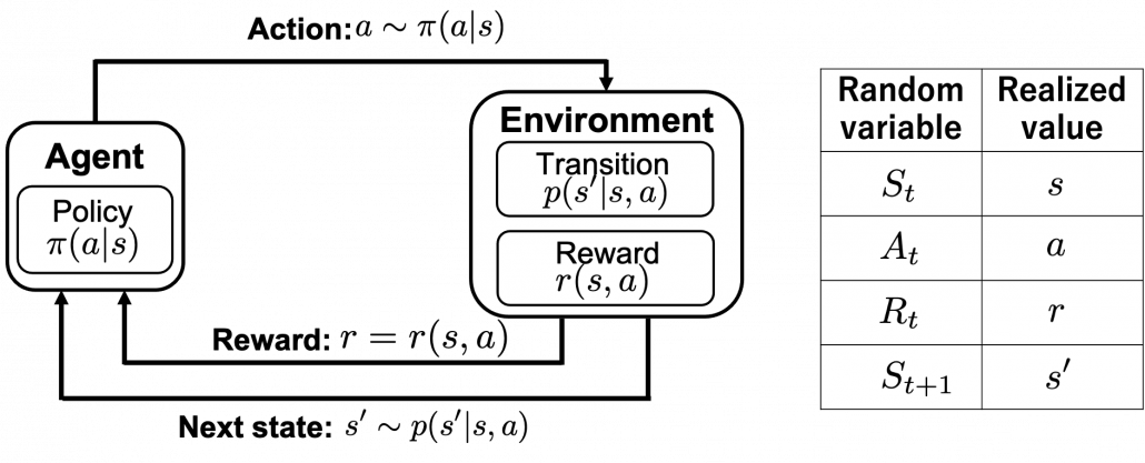
 .
.  and
and  in the chart. Actions, rewards, or transitions of states can be both deterministic or probabilistic. In the chart above, with the notation
  I meant that the action
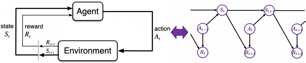
 are records of them, for example (4, 1, 6, 6, 2, 1, …). And the probability that a random variable
  . And
. And  means the random variable
  . In case
  .
. in sequential decision-making problems, usually assuming them to be MDPs. However I have to emphasize that RL is not the only way to optimize such policies. In sequential decision making problems, when the model of the environment is known, policies can be optimized also through planning without collecting data from the environment. On the other hand, when the model of the environment is unknown policies have to be optimized based on data which an agents collects from the environment through trial and errors. This is the very case called RL. You might find planning problems very simple and unrealistic in practical cases. But RL is based on planning of sequential decision-making problems with MDP settings, so studying planning problems is inevitable. As far as I could see so far, RL is a family of algorithms for approximating techniques in planning problems through trial and errors in environments. To be more concrete, in the next article I am going to explain dynamic programming (DP) in RL contexts as a major example of planning problems, and a formula called the Bellman equation plays a crucial role in planning. And after that we are going to see that RL algorithms are more or less approximations of Bellman equation by agents sampling data from environments.
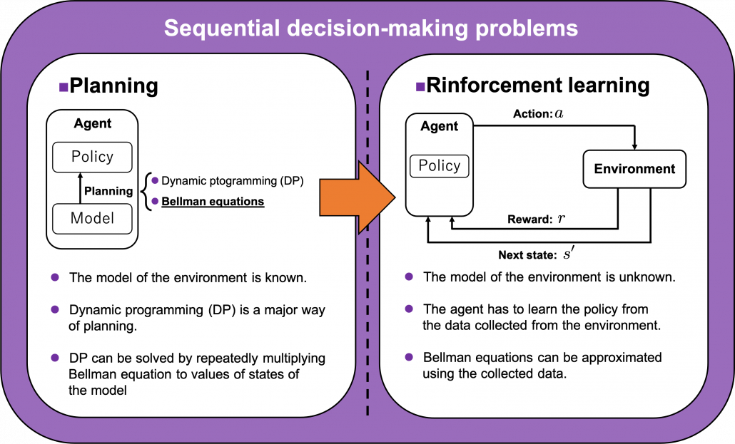
 . If the robot does not fail to take any actions or there are no unexpected obstacles, manipulating the robot on the map is a MDP. In this example, the robot has to be navigated from the start point as the green dot to the goal as the red dot. In this case, blue arrows can be obtained through planning or RL. Each blue arrow denotes the action taken in each place, following the estimated policy. In other words, the function
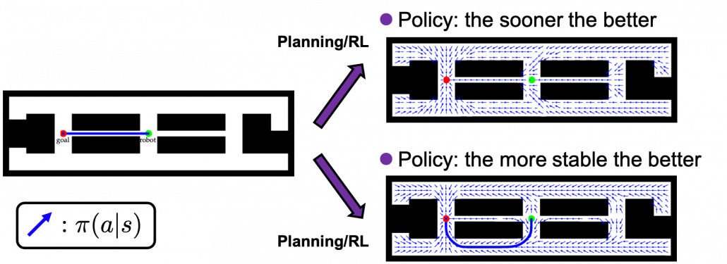
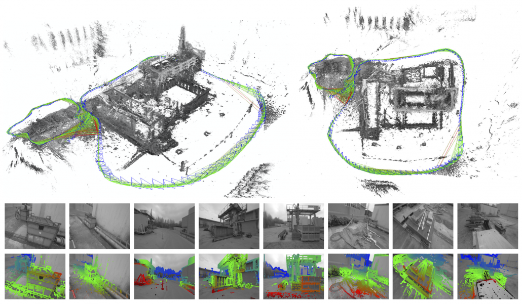
 , where
  . The
. The  is called a return. But you usually have to consider uncertainty of future rewards, so in practice you multiply a discount rate
  with rewards every time step. Thus in practice agents estimate a discounted return every time step as follows.
 directly into consideration. These rewards have to be calculated recursively and probabilistically every time step. To be exact values of states are calculated this way. The value of a state in contexts of RL mean how likely agents get higher values if they start from the state. And how to calculate values is formulated as the Bellman equation.
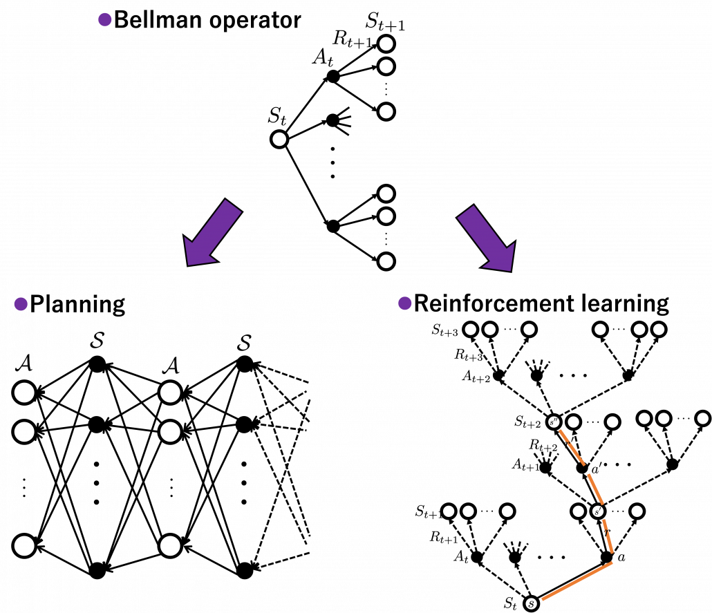
 are locations where an agent can move. Rewards
  are goals or bonuses the agents get in the course of the maze. And in this case
  .
.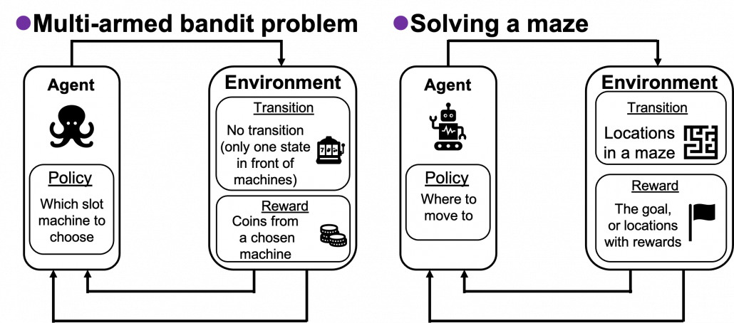
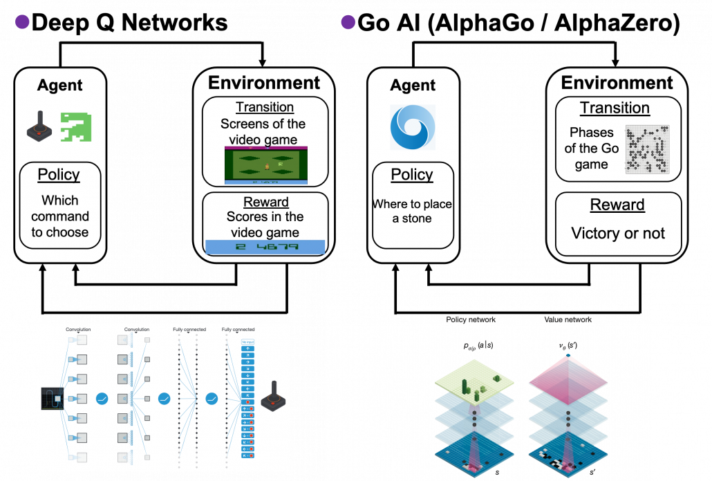
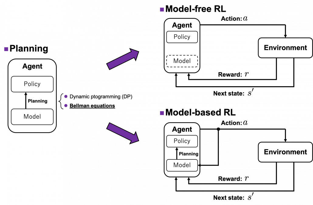
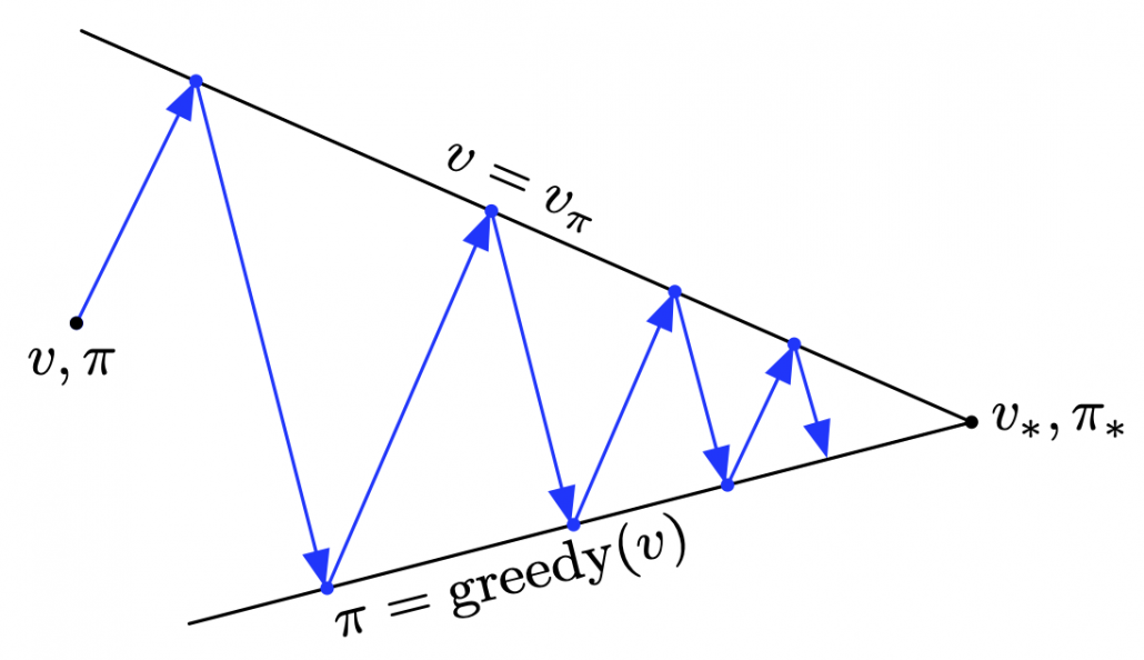
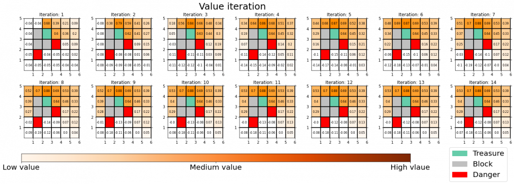
 . The number of trials is limited, so the agent has to find the machine which gives out coins the most efficiently within the limited number of trials. In this problem, the key is the balance of trying to find other effective slot machines and just trying to get as much coins as possible with the machine which for now seems to be the best. This is trade-off of “exploration” or “exploitation.” One simple way to implement exploration and exploitation trade-off is ɛ-greedy algorithm. This is quite simple: with a probability of
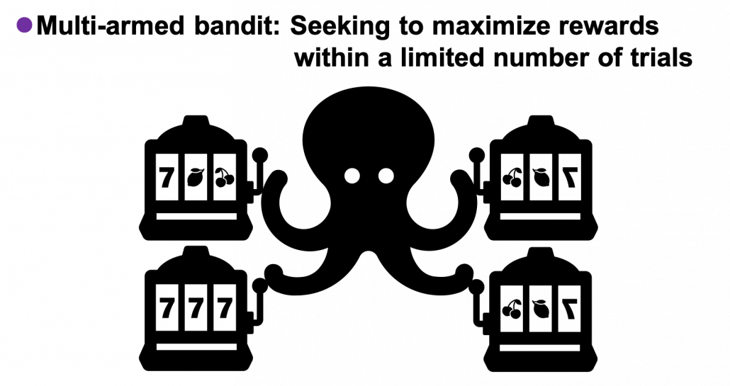
 , thus agents only need to find the machine which is the most likely to gives out more coins. But casino B is not simple like that. In this casino, slot machines with small odds give higher rewards.
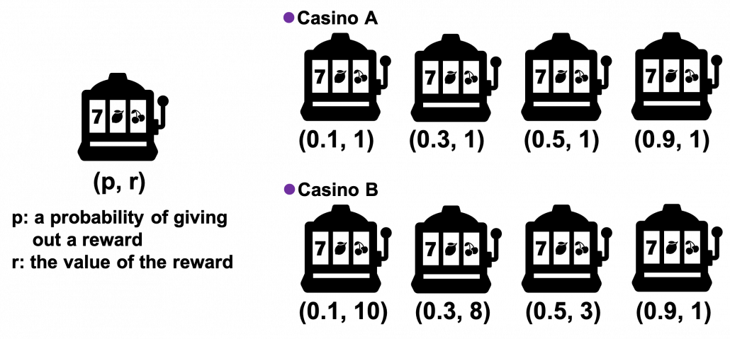
 gets the best rewards in a short term. But in the long run, more stable agent whose
  , get more rewards. On the other hand in casino B, No on seems to make outstanding results.