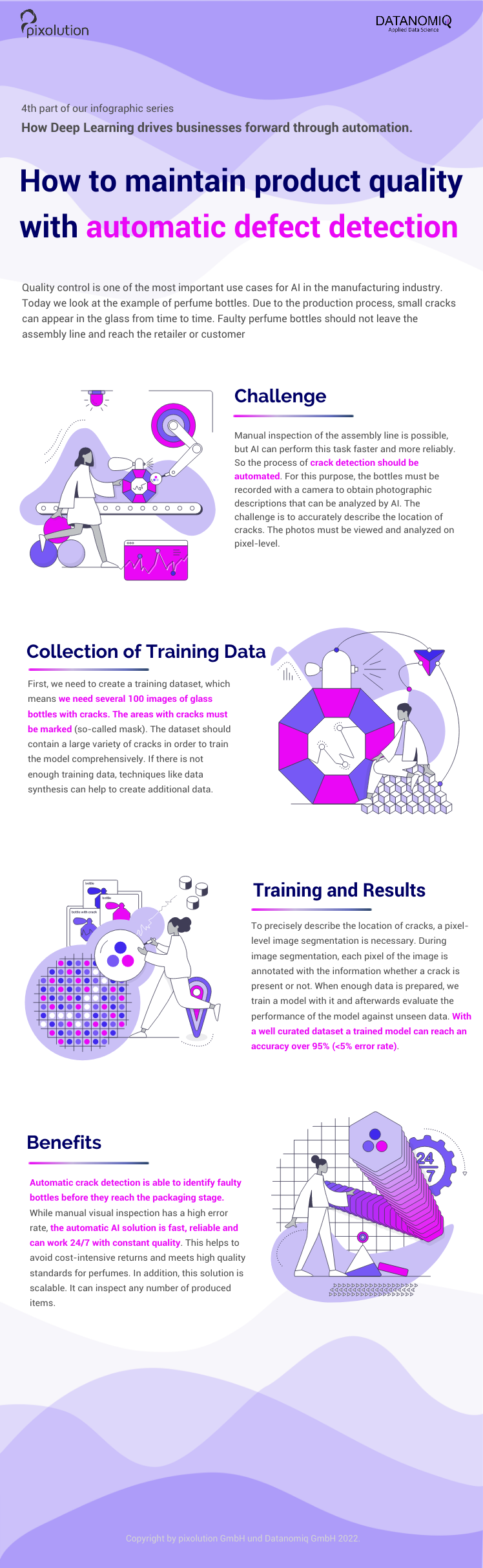
 DATANOMIQ
Data-driven Attribution Modeling
In the world of commerce, companies often face the temptation to reduce their marketing spending, especially during times of economic uncertainty or when planning to cut costs. However, this short-term strategy can lead to long-term consequences that may hinder a company’s growth and competitiveness in the market.
Maintaining a consistent marketing presence is crucial for businesses, as it helps to keep the company at the forefront of their target audience’s minds. By reducing marketing efforts, companies risk losing visibility and brand awareness among potential clients, which can be difficult and expensive to regain later. Moreover, a strong marketing strategy is essential for building trust and credibility with prospective customers, as it demonstrates the company’s expertise, values, and commitment to their industry.
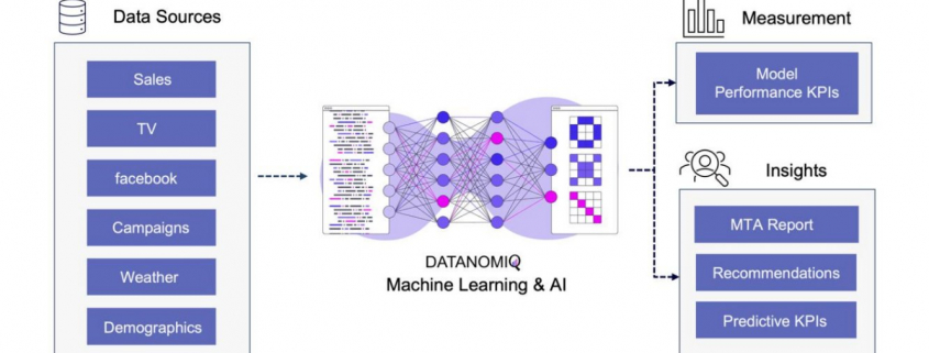
Given a fixed budget, companies apply economic principles for marketing efforts and need to spend a given marketing budget as efficient as possible. In this view, attribution models are an essential tool for companies to understand the effectiveness of their marketing efforts and optimize their strategies for maximum return on investments (ROI). By assigning optimal credit to various touchpoints in the customer journey, these models provide valuable insights into which channels, campaigns, and interactions have the greatest impact on driving conversions and therefore revenue. Identifying the most important channels enables companies to distribute the given budget accordingly in an optimal way.
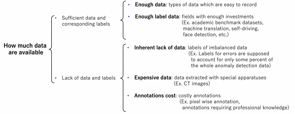
1. Combining business value with attribution modeling
The true value of attribution modeling lies not solely in applying the optimal theoretical concept – that are discussed below – but in the practical application in coherence with the business logic of the firm. Therefore, the correct modeling ensures that companies are not only distributing their budget in an optimal way but also that they incorporate the business logic to focus on an optimal long-term growth strategy.
Understanding and incorporating business logic into attribution models is the critical step that is often overlooked or poorly understood. However, it is the key to unlocking the full potential of attribution modeling and making data-driven decisions that align with business goals. Without properly integrating the business logic, even the most sophisticated attribution models will fail to provide actionable insights and may lead to misguided marketing strategies.
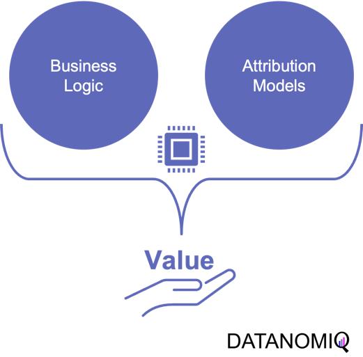
Figure 1 – Combining the business logic with attribution modeling to generate value for firms
For example, determining the end of a customer journey is a critical step in attribution modeling. When there are long gaps between customer interactions and touchpoints, analysts must carefully examine the data to decide if the current journey has concluded or is still ongoing. To make this determination, they need to consider the length of the gap in relation to typical journey durations and assess whether the gap follows a common sequence of touchpoints. By analyzing this data in an appropriate way, businesses can more accurately assess the impact of their marketing efforts and avoid attributing credit to touchpoints that are no longer relevant.
Another important consideration is accounting for conversions that ultimately lead to returns or cancellations. While it’s easy to get excited about the number of conversions generated by marketing campaigns, it’s essential to recognize that not all conversions should be valued equal. If a significant portion of conversions result in returns or cancellations, the true value of those campaigns may be much lower than initially believed.
To effectively incorporate these factors into attribution models, businesses need to important things. First, a robust data platform (such as a customer data platform; CDP) that can integrate data from various sources, such as tracking systems, ERP systems, e-commerce platforms to effectively perform data analytics. This allows for a holistic view of the customer journey, including post-conversion events like returns and cancellations, which are crucial for accurate attribution modeling. Second, as outlined above, businesses need a profound understanding of the business model and logic.
2. On the Relevance of Attribution Models in Online Marketing
A conversion is a point in the customer journey where a recipient of a marketing message performs a somewhat desired action. For example, open an email, click on a call-to-action link or go to a landing page and fill out a registration. Finally, the ultimate conversion would be of course buying the product. Attribution models serve as frameworks that help marketers assess the business impact of different channels on a customer’s decision to convert along a customer´s journey. By providing insights into which interactions most effectively drive sales, these models enable more efficient resource allocation given a fixed budget.
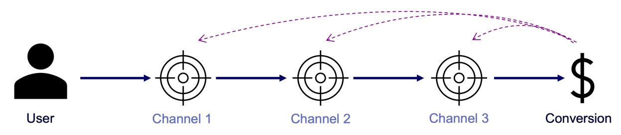
Figure 2 – A simple illustration of one single customer journey. Consider that from the company’s perspective all journeys together result into a complex network of possible journey steps.
Companies typically utilize a diverse marketing mix, including email marketing, search engine advertising (SEA), search engine optimization (SEO), affiliate marketing, and social media. Attribution models facilitate the analysis of customer interactions across these touchpoints, offering a comprehensive view of the customer journey.
-
Comprehensive Customer Insights: By identifying the most effective channels for driving conversions, attribution models allow marketers to tailor strategies that enhance customer engagement and improve conversion rates.
-
Optimized Budget Allocation: These models reveal the performance of various marketing channels, helping marketers allocate budgets more efficiently. This ensures that resources are directed towards channels that offer the highest return on investment (ROI), maximizing marketing impact.
-
Data-Driven Decision Making: Attribution models empower marketers to make informed, data-driven decisions, leading to more effective campaign strategies and better alignment between marketing and sales efforts.
In the realm of online advertising, evaluating media effectiveness is a critical component of the decision-making process. Since advertisement costs often depend on clicks or impressions, understanding each channel’s effectiveness is vital. A multi-channel attribution model is necessary to grasp the marketing impact of each channel and the overall effectiveness of online marketing activities. This approach ensures optimal budget allocation, enhances ROI, and drives successful marketing outcomes.
What types of attribution models are there? Depending on the attribution model, different values are assigned to various touchpoints. These models help determine which channels are the most important and should be prioritized. Each channel is assigned a monetary value based on its contribution to success. This weighting then determines the allocation of the marketing budget. Below are some attribution models commonly used in marketing practice.
2.1. Single-Touch Attribution Models
As it follows from the name of the group of these approaches, they consider only one touchpoint.
2.1.1 First Touch Attribution
First touch attribution is the standard and simplest method for attributing conversions, as it assigns full credit to the first interaction. One of its main advantages is its simplicity; it is a straightforward and easy-to-understand approach. Additionally, it allows for quick implementation without the need for complex calculations or data analysis, making it a convenient choice for organizations looking for a simple attribution method. This model can be particularly beneficial when the focus is solely on demand generation. However, there are notable drawbacks to first touch attribution. It tends to oversimplify the customer journey by ignoring the influence of subsequent touchpoints. This can lead to a limited view of channel performance, as it may disproportionately credit channels that are more likely to be the first point of contact, potentially overlooking the contributions of other channels that assist in conversions.
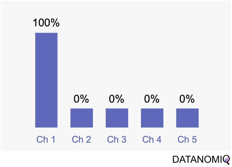
Figure 3 – The first touch is a simple non-intelligent way of attribution.
2.1.2 Last Touch Attribution
Last touch attribution is another straightforward method for attributing conversions, serving as the opposite of first touch attribution by assigning full credit to the last interaction. Its simplicity is one of its main advantages, as it is easy to understand and implement without the need for complex calculations or data analysis. This makes it a convenient choice for organizations seeking a simple attribution approach, especially when the focus is solely on driving conversions. However, last touch attribution also has its drawbacks. It tends to oversimplify the customer journey by neglecting the influence of earlier touchpoints. This approach provides limited insights into the full customer journey, as it focuses solely on the last touchpoint and overlooks the cumulative impact of multiple touchpoints, missing out on valuable insights.
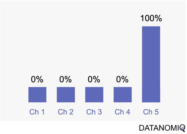
Figure 4 – Last touch attribution is the counterpart to the first touch approach.
2.2 Multi-Touch Attribution Models
We noted that single-touch attribution models are easy to interpret and implement. However, these methods often fall short in assigning credit, as they apply rules arbitrarily and fail to accurately gauge the contribution of each touchpoint in the consumer journey. As a result, marketers may make decisions based on skewed data. In contrast, multi-touch attribution leverages individual user-level data from various channels. It calculates and assigns credit to the marketing touchpoints that have influenced a desired business outcome for a specific key performance indicator (KPI) event.
2.2.1 Linear Attribution
Linear attribution is a standard approach that improves upon single-touch models by considering all interactions and assigning them equal weight. For instance, if there are five touchpoints in a customer’s journey, each would receive 20% of the credit for the conversion. This method offers several advantages. Firstly, it ensures equal distribution of credit across all touchpoints, providing a balanced representation of each touchpoint’s contribution to conversions. This approach promotes fairness by avoiding the overemphasis or neglect of specific touchpoints, ensuring that credit is distributed evenly among channels. Additionally, linear attribution is easy to implement, requiring no complex calculations or data analysis, which makes it a convenient choice for organizations seeking a straightforward attribution method. However, linear attribution also has its drawbacks. One significant limitation is its lack of differentiation, as it assigns equal credit to each touchpoint regardless of their actual impact on driving conversions. This can lead to an inaccurate representation of the effectiveness of individual touchpoints. Furthermore, linear attribution ignores the concept of time decay, meaning it does not account for the diminishing influence of earlier touchpoints over time. It treats all touchpoints equally, regardless of their temporal proximity to the conversion event, potentially overlooking the greater impact of more recent interactions.
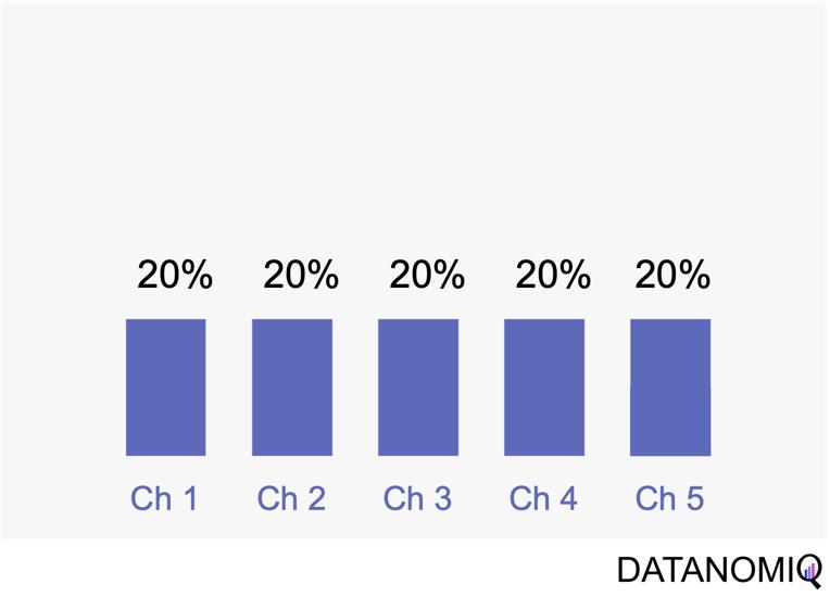
Figure 5 – Linear uniform attribution.
2.2.2 Position-based Attribution (U-Shaped Attribution & W-Shaped Attribution)
Position-based attribution, encompassing both U-shaped and W-shaped models, focuses on assigning the most significant weight to the first and last touchpoints in a customer’s journey. In the W-shaped attribution model, the middle touchpoint also receives a substantial amount of credit. This approach offers several advantages. One of the primary benefits is the weighted credit system, which assigns more credit to key touchpoints such as the first and last interactions, and sometimes additional key touchpoints in between. This allows marketers to highlight the importance of these critical interactions in driving conversions. Additionally, position-based attribution provides flexibility, enabling businesses to customize and adjust the distribution of credit according to their specific objectives and customer behavior patterns. However, there are some drawbacks to consider. Position-based attribution involves a degree of subjectivity, as determining the specific weights for different touchpoints requires subjective decision-making. The choice of weights can vary across organizations and may affect the accuracy of the attribution results. Furthermore, this model has limited adaptability, as it may not fully capture the nuances of every customer journey, given its focus on specific positions or touchpoints.
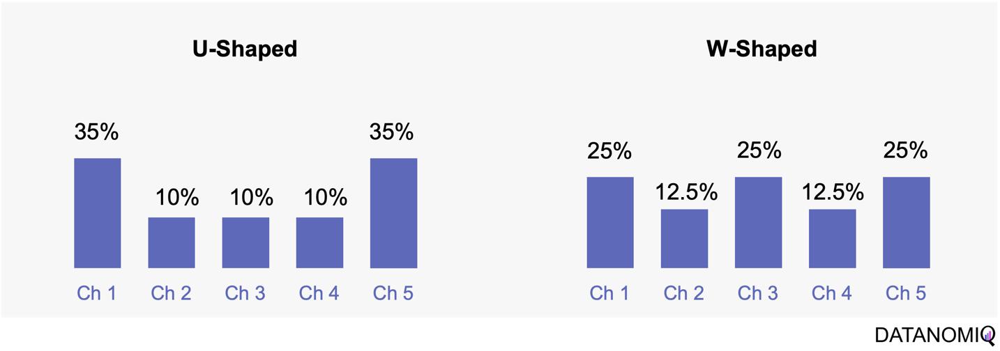
Figure 6 – The U-shaped attribution (sometimes known as “bathtube model” and the W-shaped one are first attempts of weighted models.
2.2.3 Time Decay Attribution
Time decay attribution is a model that primarily assigns most of the credit to interactions that occur closest to the point of conversion. This approach has several advantages. One of its key benefits is temporal sensitivity, as it recognizes the diminishing impact of earlier touchpoints over time. By assigning more credit to touchpoints closer to the conversion event, it reflects the higher influence of recent interactions. Additionally, time decay attribution offers flexibility, allowing organizations to customize the decay rate or function. This enables businesses to fine-tune the model according to their specific needs and customer behavior patterns, which can be particularly useful for fast-moving consumer goods (FMCG) companies. However, time decay attribution also has its drawbacks. One challenge is the arbitrary nature of the decay function, as determining the appropriate decay rate is both challenging and subjective. There is no universally optimal decay function, and choosing an inappropriate model can lead to inaccurate credit distribution. Moreover, this approach may oversimplify time dynamics by assuming a linear or exponential decay pattern, which might not fully capture the complex temporal dynamics of customer behavior. Additionally, time decay attribution primarily focuses on the temporal aspect and may overlook other contextual factors that influence touchpoint effectiveness, such as channel interactions, customer segments, or campaign-specific dynamics.
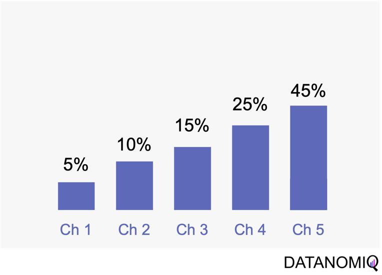
Figure 7 – Time-based models can be configurated by according to the first or last touch and weighted by the timespan in between of each touchpoint.
2.3 Data-Driven Attribution Models
2.3.1 Markov Chain Attribution
Markov chain attribution is a data-driven method that analyzes marketing effectiveness using the principles of Markov Chains. Those chains are mathematical models used to describe systems that transition from one state to another in a chain-like process. The principles focus on the transition matrix, derived from analyzing customer journeys from initial touchpoints to conversion or no conversion, to capture the sequential nature of interactions and understand how each touchpoint influences the final decision. Let’s have a look at the following simple example with three channels that are chained together and leading to either a conversion or no conversion.
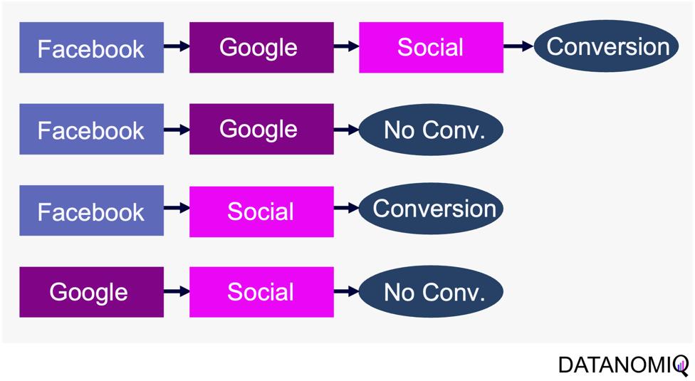
Figure 8 – Example of four customer journeys
The model calculates the conversion likelihood by examining transitions between touchpoints. Those transitions are depicted in the following probability tree.
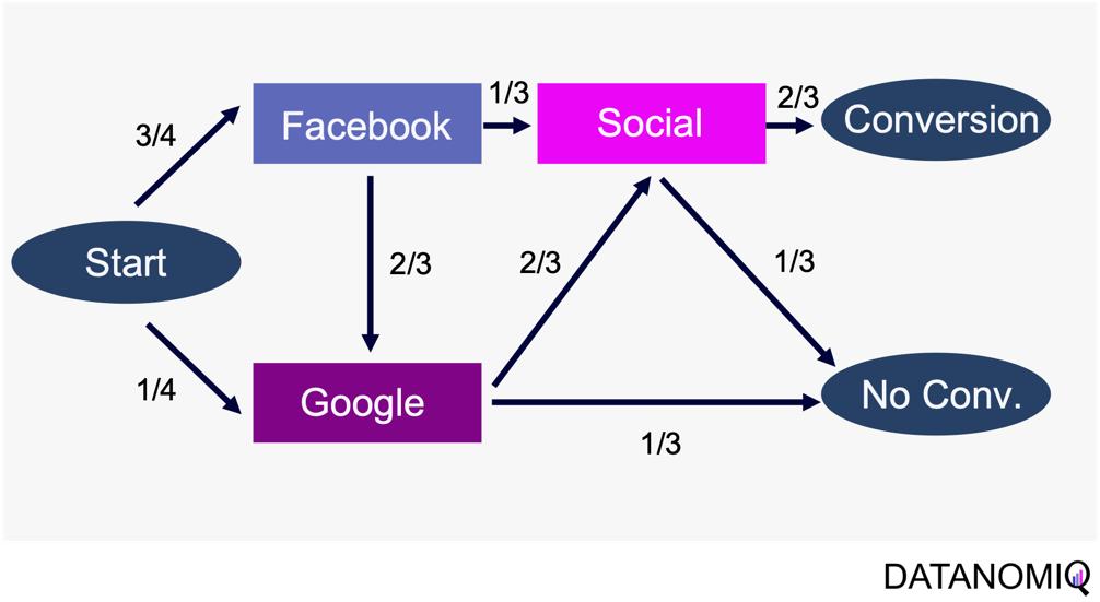
Figure 9 – Example of a touchpoint network based on customer journeys
Based on this tree, the transition matrix can be constructed that reveals the influence of each touchpoint and thus the significance of each channel.
This method considers the sequential nature of customer journeys and relies on historical data to estimate transition probabilities, capturing the empirical behavior of customers. It offers flexibility by allowing customization to incorporate factors like time decay, channel interactions, and different attribution rules.
Markov chain attribution can be extended to higher-order chains, where the probability of transition depends on multiple previous states, providing a more nuanced analysis of customer behavior. To do so, the Markov process introduces a memory parameter 0 that is assumed to be zero here. Overall, it offers a robust framework for understanding the influence of different marketing touchpoints.
2.3.2 Shapley Value Attribution (Game Theoretical Approach)
The Shapley value is a concept from game theory that provides a fair method for distributing rewards among participants in a coalition. It ensures that both gains and costs are allocated equitably among actors, making it particularly useful when individual contributions vary but collective efforts lead to a shared outcome. In advertising, the Shapley method treats the advertising channels as players in a cooperative game. Now, consider a channel coalition consisting of different advertising channels . The utility function describes the contribution of a coalition of channels .
In this formula, is the cardinality of a specific coalition and the sum extends over all subsets of that do not contain the marginal contribution of channel to the coalition . For more information on how to calculate the marginal distribution, see Zhao et al. (2018).
The Shapley value approach ensures a fair allocation of credit to each touchpoint based on its contribution to the conversion process. This method encourages cooperation among channels, fostering a collaborative approach to achieving marketing goals. By accurately assessing the contribution of each channel, marketers can gain valuable insights into the performance of their marketing efforts, leading to more informed decision-making. Despite its advantages, the Shapley value method has some limitations. The method can be sensitive to the order in which touchpoints are considered, potentially leading to variations in results depending on the sequence of attribution. This sensitivity can impact the consistency of the outcomes. Finally, Shapley value and Markov chain attribution can also be combined using an ensemble attribution model to further reduce the generalization error (Gaur & Bharti 2020).
2.33. Algorithmic Attribution using binary Classifier and (causal) Machine Learning
While customer journey data often suffices for evaluating channel contributions and strategy formulation, it may not always be comprehensive enough. Fortunately, companies frequently possess a wealth of additional data that can be leveraged to enhance attribution accuracy by using a variety of analytics data from various vendors. For examples, companies might collect extensive data, including customer website activity such as clicks, page views, and conversions. This data includes features like for example the Urchin Tracking Module (UTM) information such as source, medium, campaign, content and term as well as campaign, device type, geographical information, number of user engagements, and scroll frequency, among others.
Utilizing this information, a binary classification model can be trained to predict the probability of conversion at each step of the multi touch attribution (MTA) model. This approach not only identifies the most effective channels for conversions but also highlights overvalued channels. Common algorithms include logistic regressions to easily predict the probability of conversion based on various features. Gradient boosting also provides a popular ensemble technique that is often used for unbalanced data, which is quite common in attribution data. Moreover, random forest models as well as support vector machines (SVMs) are also frequently applied. When it comes to deep learning models, that are often used for more complex problems and sequential data, Long Short-Term Memory (LSTM) networks or Transformers are applied. Those models can capture the long-range dependencies among multiple touchpoints.
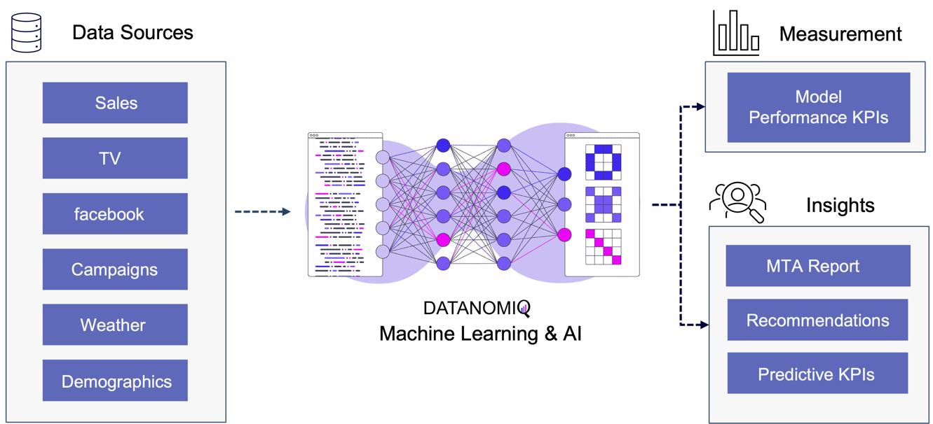
Figure 10 – Attribution Model based on Deep Learning / AI
The approach is scalable, capable of handling large volumes of data, making it ideal for organizations with extensive marketing campaigns and complex customer journeys. By leveraging advanced algorithms, it offers more accurate attribution of credit to different touchpoints, enabling marketers to make informed, data-driven decisions.
All those models are part of the Machine Learning & AI Toolkit for assessing MTA. And since the business world is evolving quickly, newer methods such as double Machine Learning or causal forest models that are discussed in the marketing literature (e.g. Langen & Huber 2023) in combination with eXplainable Artificial Intelligence (XAI) can also be applied as well in the DATANOMIQ Machine Learning and AI framework.
3. Conclusion
As digital marketing continues to evolve in the age of AI, attribution models remain crucial for understanding the complex customer journey and optimizing marketing strategies. These models not only aid in effective budget allocation but also provide a comprehensive view of how different channels contribute to conversions. With advancements in technology, particularly the shift towards data-driven and multi-touch attribution models, marketers are better equipped to make informed decisions that enhance quick return on investment (ROI) and maintain competitiveness in the digital landscape.
Several trends are shaping the evolution of attribution models. The increasing use of machine learning in marketing attribution allows for more precise and predictive analytics, which can anticipate customer behavior and optimize marketing efforts accordingly. Additionally, as privacy regulations become more stringent, there is a growing focus on data quality and ethical data usage (Ethical AI), ensuring that attribution models are both effective and compliant. Furthermore, the integration of view-through attribution, which considers the impact of ad impressions that do not result in immediate clicks, provides a more holistic understanding of customer interactions across channels. As these models become more sophisticated, they will likely incorporate a wider array of data points, offering deeper insights into the customer journey.
Unlock your marketing potential with a strategy session with our DATANOMIQ experts. Discover how our solutions can elevate your media-mix models and boost your organization by making smarter, data-driven decisions.
References
- Zhao, K., Mahboobi, S. H., & Bagheri, S. R. (2018). Shapley value methods for attribution modeling in online advertising. arXiv preprint arXiv:1804.05327.
- Gaur, J., & Bharti, K. (2020). Attribution modelling in marketing: Literature review and research agenda. Academy of Marketing Studies Journal, 24(4), 1-21.
- Langen H, Huber M (2023) How causal machine learning can leverage marketing strategies: Assessing and improving the performance of a coupon campaign. PLoS ONE 18(1): e0278937. https://doi.org/10.1371/journal. pone.0278937
 by adjusting parameters
  . And the parameters
  is minimized. If it is a supervised learning, the a value of a loss function is denoted
 , and it gets smaller as
  gets closer to
  . That is,
  via
via  . And in a case of unsupervised learning, a loss function is
  , which is often heuristically handcrafted.
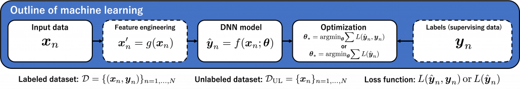
 of a butterfly below with a label of
  can be converted to more than 6 images. This corresponds to getting a converted
  in the machine learning outline in the last section. And this process is the same as increasing the size of a dataet
  . And one point you have to be careful is, you must not change
  Here let me take an example of data augmentation technique that would be contrary to your intuition. A technique named mixup literally mix up data with different classes and their labels. In classification problems, labels are expressed as one-hot vectors, that is only an element corresponding to a correct element is
  and the others are
  . In a case of binary dog-or-cat classification, each label is
  or
or  , respectively. In data augmentation, distorting data too much is a taboo because label data is contaminated, but in mixup you literally mix up labels. Randomly choosing a two inputs
  and a number
 ![\lambda \in [0,1]](https://data-science-blog.com/en/wp-content/ql-cache/quicklatex.com-ca07e0e397d614f2de6877183c93fa3a_l3.png "Rendered by QuickLaTeX.com") , you prepare a input and label pair
, you prepare a input and label pair  . The figure below is an example of a mixing up a cat input and a dog input, and corresponding labels. It is known augmenting training data like this improves classification performances. It is said this is partly due to machine learning models effectively learning decision boundaries. In classification ambiguous inputs are bottlenecks, so learning to giving ambiguous outputs to ambiguous inputs can enhance classification abilities.
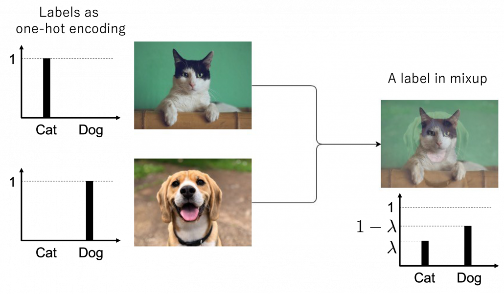
 for a
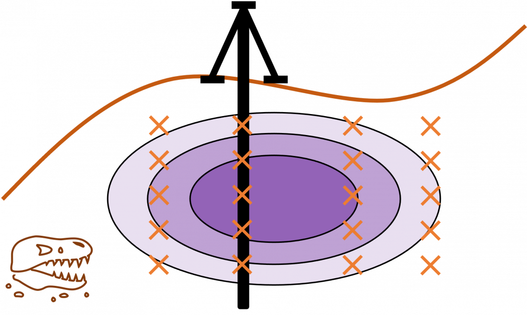
for a  . When you want to regress the data with as few samples as possible, data points should be sampled from the parts with great uncertainties. And by doing so, you can see that the data is regressed efficiently with few samples.
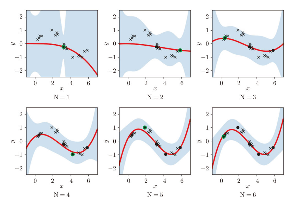
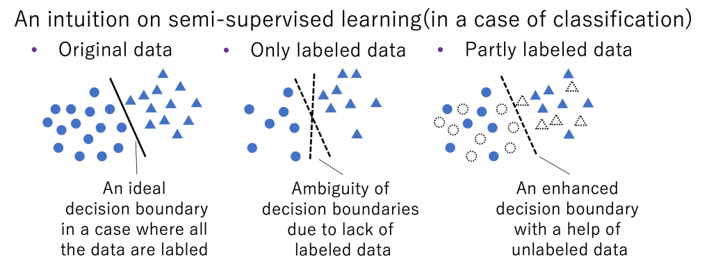
 for a labeled dataset
  . In semi-supervised learning, we assume that usually a bigger unsupervised dataset
  is available in the same domain. And semi-supervised learning optimize
  after designing a loss function
  for the unlabeled dataset. There are following 3 major ways of semi-supervised learning depending on how you design a
  in
in  . And training
  and
and  give out a consistent output.
 images in a dataset with a pre-trained backbone CNN, and I got corresponding
  dimensional vectors, that is a
  tensor. And I applied t-SNE to reduce its dimension from
  and got a
  tensor. The figure below shows arrangements of input images in the 2 dimensional space. As you can see, semantically similar images get closer.

 , which effective for each task.
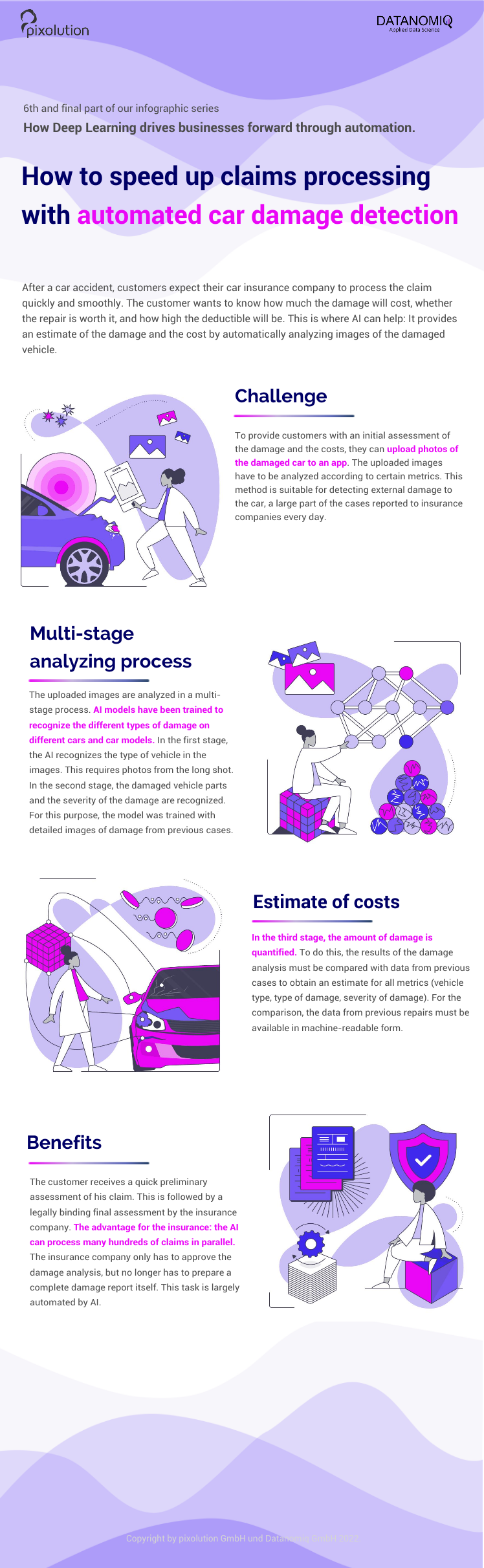


 in an state space
  , and black nodes representing each action
  , which is a member of an action space
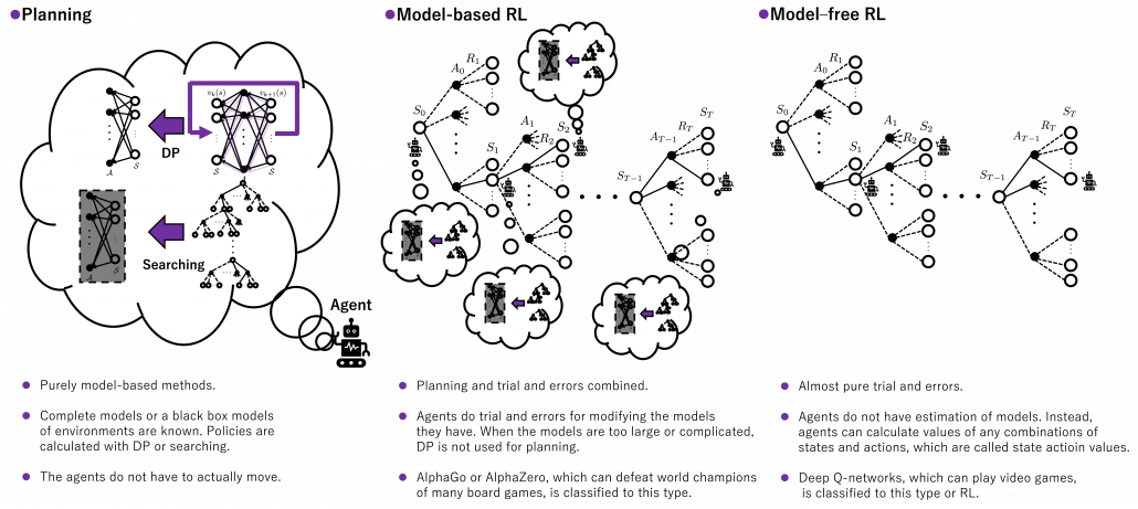
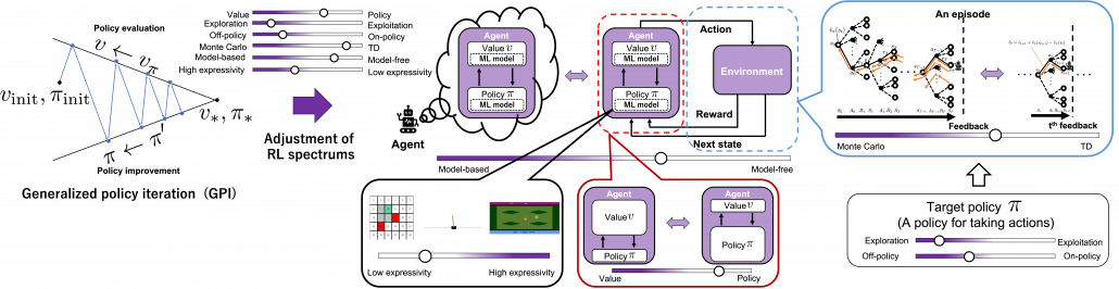
  . Any behaviors of agents are represented as going back and forth between black and white nodes of the model, and that is why connections in the MDP model are bidirectional. In my articles let me call such model of environments “a closed model.” RL or general planning problems are matters of optimizing policies in such models of environments. Optimizing the policies are roughly classified into two types, planning/searching or RL, and the main difference between them is whether connections of graphs of models are known or not. Planning or searching is conducted without actually moving in the environment. DP are family of planning algorithms which are known to converge, and so far in my articles we have seen that DP are enabled by repeatedly applying Bellman operators. But instead of considering and updating all the possible transitions in the model like DP, planning can be conducted more sparsely. Such sparse planning are often called searching, and many of them use tree structures. If you have learned any general decision making problems with tree graphs, you might be already familiar with some searching techniques like alpha-beta pruning.
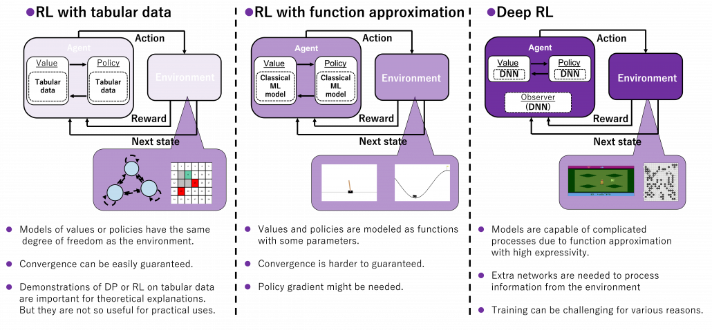
 , in MDPs. Other general machine learning algorithms have more direct supervision by loss functions and models are optimized so that loss functions are minimized. In the case of the figure below, an ML model
  is optimized to
  by optimization such as gradient descent. But on the other hand in RL policies
  do not have direct loss functions. Then RL uses values
  , which are functions of how good it is to be in states
  for the current policy
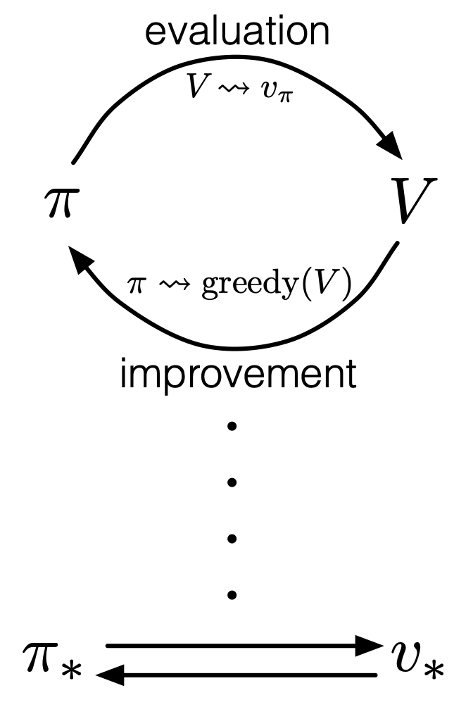
  , which is called policy improvement, and overall processes of estimation and policy improvement are called control in the book. And
  or policies
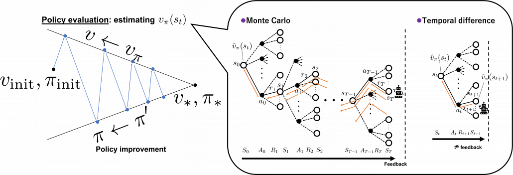
  . This interactive updates of values and policies are done inside the agent, in the dotted frame in red below. I personally think this part should be more emphasized than trial-and-error-like behaviors of agents. Once you see trial and errors of RL as crucial but just one aspect of GPI and focus more inside agents, you would see why so many study materials start explaining RL with DP.
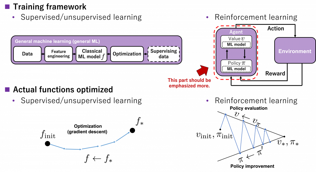
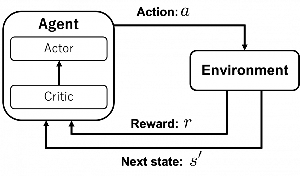
 , randomness of actions can be also learned by modeling policies with certain functions. This randomness of functions can be also modeled in actor-critic frameworks. That means, depending on a choice of an actor, such actor can learn randomness of actions, that is explorations.

 , and gives out the next state
  and corresponding reward
  , that is the black box is a sample model. In this case other planning methods with some searching algorithms are used, for example Monte Carlo tree search. Such search algorithms are designed to more efficiently and sparsely search states and actions of interest. Many of searching algorithms used in RL make uses of tree structures. Model-based approaches can be roughly classified into three types below based on size or complication of models.
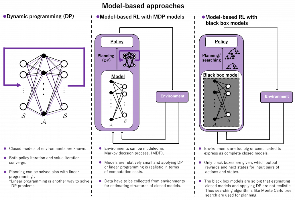
 *And this spectrum is also a spectrum of computation costs or convergence. The left type could be easily implemented like programming assignments of schools since it in short needs only Excel sheets, and you would soon get results. The middle type would be more challenging, but that would not b computationally too expensive. But when it comes to the type at the right side, that is not something which should be done on your local computer. At least you need a GPU. You should expect some hours or days even for training RL agents to play 8 bit video games. That is of course due to cost of training deep neural networks (DNN), especially CNN. But another factors is potential inefficiency of RL. I hope I could explain those weak points of RL and remedies for them.

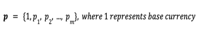
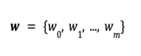
 , the total value
  of the portfolio is defined as the inner product of the price vector
  and the portfolio vector
  .
. at the terminal time step
  .
.
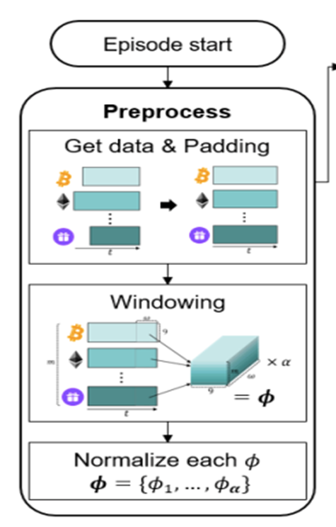
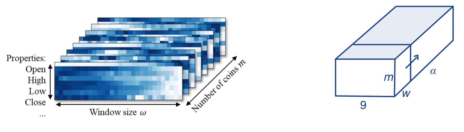
 ) is stored in the repository as a sample of training data.
 is defined as the softmax value for the q-value of each action (ie. i-th asset at
  , then i-th asset is bought using 50% of base currency).
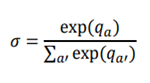
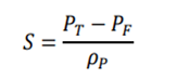
 is the return of a risk-free asset, which is set to 0 here.
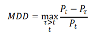
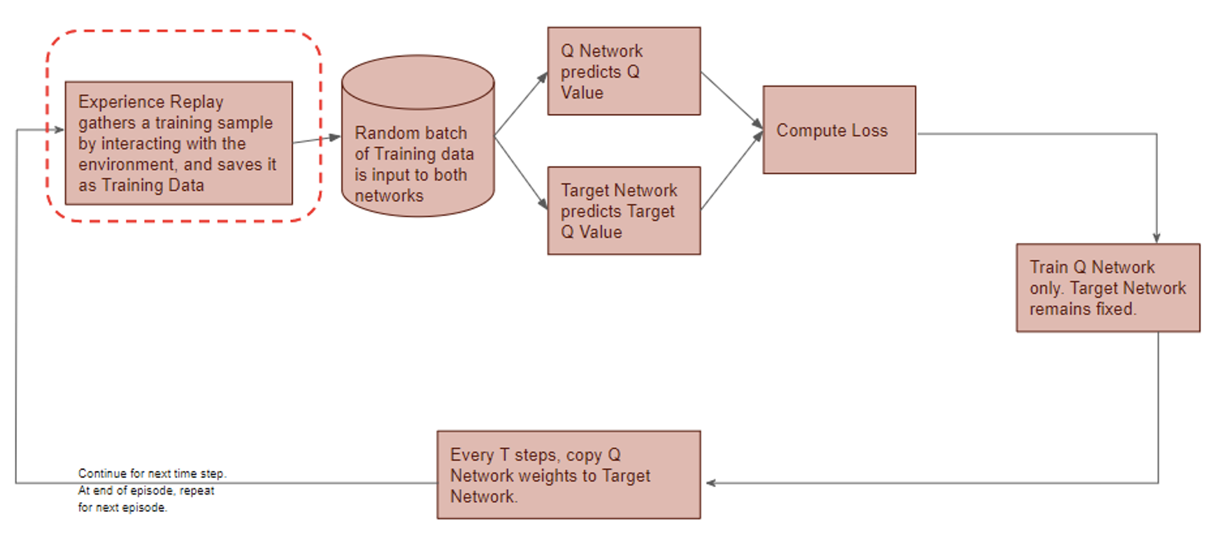
 are initialized to 0, while the policy π(s) is uniformly distributed among all actions. Afterwards, everything is updated through interacting with the stock market environment. By the Bellman Equation,
  is the expectation of the sum of direct reward
  and the future reqard
  at the next state discounted by a factor γ, resulting in the state-action value function:
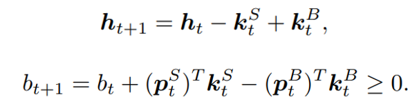
![[b_t, p_t, h_t, M_t, R_t, C_t, X_t]](https://data-science-blog.com/en/wp-content/ql-cache/quicklatex.com-0fbdf800e4e901e62bc4396f3815d15f_l3.png "Rendered by QuickLaTeX.com") storing information about
storing information about : Portfolio balance
 : Shares owned of each stock
 : Moving Average Convergence Divergence
 : Relative Strength Index
 : Commodity Channel Index
 : Average Directional Index
 is the policy network, and
  is the advantage function to reduce the high variance of it:
 is the value function of state
  , regardless of actions. DDPG: combines the frameworks of Q-learning and policy gradients and uses neural networks as function approximators; it learns directly from the observations through policy gradient and deterministically map states to actions. The Q-value is updated by:

 and produces a sample that has a similar distribution as
  . To train this network efficiently, there is the other network that is utilized as the second player and known as the discriminator. The generator network (player one) tries to fool the discriminator by generating real looking images. Moreover, the discriminator network tries to distinguish between real (training data
  ) and fake images effectively. Our main aim is to have an efficiently trained discriminator to be able to distinguish between real and fake images (the generator’s output) and on the other hand, we would like to have a generator, which can easily fool the discriminator by generating real-looking images.
![\begin{equation*} \min_{p_{\theta_g}}\: \max_{D_{\theta_d}\in F} \: \mathbb{E}_{x\sim p_d}[D_{\theta_d}(x)] - \mathbb{E}_{x\sim p_{\theta_g}} [D_{\theta_d}(G_{\theta_g}(x))], \end{equation*}](https://data-science-blog.com/en/wp-content/ql-cache/quicklatex.com-7980edcee550a3814c1f817f58e1bfb3_l3.png "Rendered by QuickLaTeX.com")
 and
and  is a set of functions. The \textit{max} part is computing the discrepancies between two distribution using a function
  and this part is very similar to the term
  (discrepancy measure) from our
  . The above mentioned objective function does not use any likelihood function and utilizing two different data samples from training and generated data respectively.
![\mathbb{E}_{x\sim p_d}[D_{\theta_d}(x)]](https://data-science-blog.com/en/wp-content/ql-cache/quicklatex.com-1c4b4cb35296fdd7dc76bf9166842c48_l3.png "Rendered by QuickLaTeX.com") corresponds to the discriminator, which has direct access to the training data and the second term
corresponds to the discriminator, which has direct access to the training data and the second term ![\mathbb{E}_{x\sim p_{\theta_g}}[D_{\theta_d}(G_{\theta_g}(x))]](https://data-science-blog.com/en/wp-content/ql-cache/quicklatex.com-9271a567a190dfafd06b4f7d53f5ffa8_l3.png "Rendered by QuickLaTeX.com") represents the generator part as it relies only on the latent space and produces synthetic data. Therefore, Equation
represents the generator part as it relies only on the latent space and produces synthetic data. Therefore, Equation ![\begin{equation*} \min_{p_{\theta_g}}\: \max_{D_{\theta_d}\in F} \: \mathbb{E}_{x\sim p_d}[D_{\theta_d}(x)] - \mathbb{E}_{z\sim p_z}[D_{\theta_d}(G_{\theta_g}(z))], \end{equation*}](https://data-science-blog.com/en/wp-content/ql-cache/quicklatex.com-768b9dece98731bd7d56aaa85d15a3d9_l3.png "Rendered by QuickLaTeX.com")
![\begin{equation*} \min_{\theta_g}\: \max_{\theta_d} \: (\mathbb{E}_{x\sim p_d} [log \: D_{\theta_d} (x)] + \mathbb{E}_{z\sim p_z}[log(1 - D_{\theta_d}(G_{\theta_g}(z))]), \end{equation*}](https://data-science-blog.com/en/wp-content/ql-cache/quicklatex.com-bac04040928a64b0805eb863ec4e2864_l3.png "Rendered by QuickLaTeX.com")
 to
to  and
and  respectively as we would like to approximate the network parameters, which are represented by
  , which indicates that the outcome is close to the real data. Furthermore,
  should be close to zero as it is fake data, therefore, the maximization of the above objective function for
  . If the minimization of the objective function happens effectively for
  is a random input vector to the generator to produce a synthetic outcome
  (green curve). The generated data distribution is not close to the original data distribution
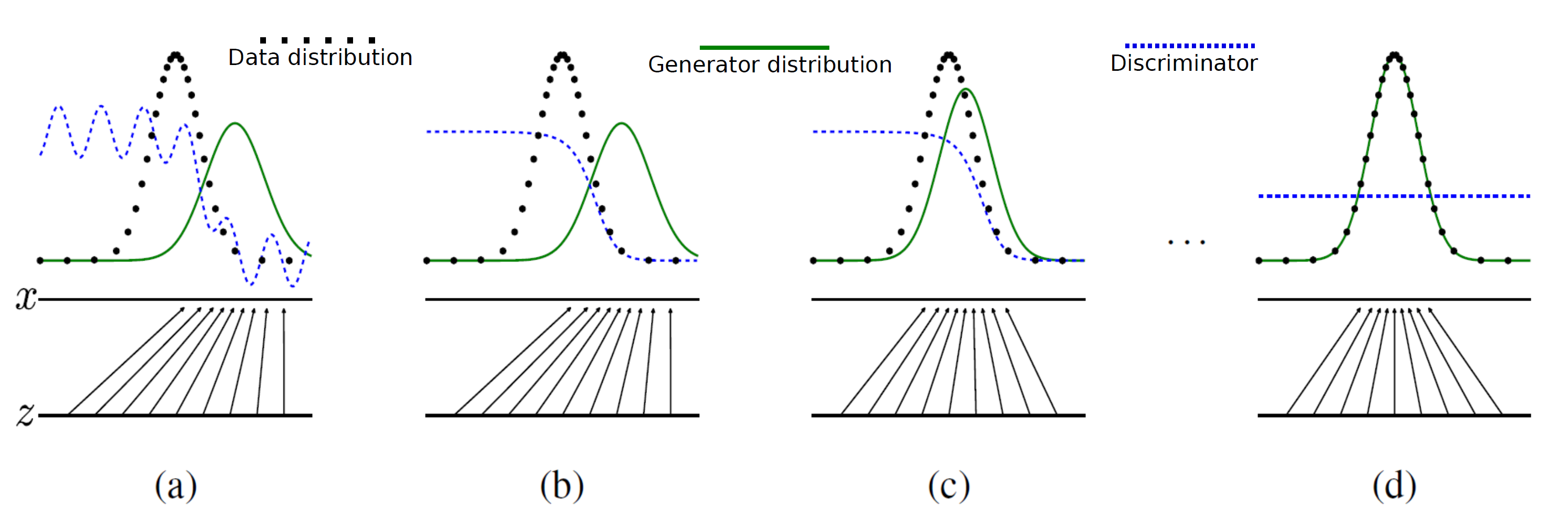
![\begin{equation*} \max_{\theta_d} \: (\mathbb{E}_{x\sim p_d} [log \: D_{\theta_d}(x)] + \mathbb{E}_{z\sim p_z}[log(1 - D_{\theta_d}(G_{\theta_g}(z))]) \end{equation*}](https://data-science-blog.com/en/wp-content/ql-cache/quicklatex.com-79cc0abf65c2730d44630b9e9078c251_l3.png "Rendered by QuickLaTeX.com")
![\begin{equation*} \min_{\theta_g} \: ( \mathbb{E}_{z\sim p_z}[log(1 - D_{\theta_d}(G_{\theta_g}(z))]) \end{equation*}](https://data-science-blog.com/en/wp-content/ql-cache/quicklatex.com-1a5f55cfe2aa160fc40a567edc93237d_l3.png "Rendered by QuickLaTeX.com")
 then the term
  has the dominant gradient and vice versa.
 , the generator is not well trained and producing low quality outputs therefore, it requires a dominant gradient for an efficient training. To fix this problem, the gradient ascent method is applied to maximize the modified generator’s objective:
![\begin{equation*} \max_{\theta_g} \: \mathbb{E}_{z\sim p_z}[log \: (D_{\theta_d}(G_{\theta_g}(z))] \end{equation*}](https://data-science-blog.com/en/wp-content/ql-cache/quicklatex.com-20421f265a98722e9835849d78d80269_l3.png "Rendered by QuickLaTeX.com")


 produces meaningful information of
  .
.

 to approximate the conditional
  to generate images based on a sample from a true prior,
  are generally of Gaussian distribution.
 as it will be performing probabilistic generation of data. Therefore the encoder and decoder should be probabilistic.
 prior distribution, which is a Gaussian function, therefore, both of them are tractable. However, the integration won’t be tractable because of the high dimensionality of data.
 to approximate the conditional
  . Furthermore, the conditional
  , which is intractable. This additional encoder part will help to derive a lower bound on the data likelihood that will make the likelihood function tractable. In the following we will derive the lower bound of the likelihood function:
![\begin{equation*} \begin{flalign} \begin{aligned} log \: p_\theta (x) = & \mathbf{E}_{z\sim q_\phi(z|x)} \Bigg[log \: \frac{p_\theta (x|z) p_\theta (z)}{p_\theta (z|x)} \: \frac{q_\phi(z|x)}{q_\phi(z|x)}\Bigg] \\ = & \mathbf{E}_{z\sim q_\phi(z|x)} \Bigg[log \: p_\theta (x|z)\Bigg] - \mathbf{E}_{z\sim q_\phi(z|x)} \Bigg[log \: \frac{q_\phi (z|x)} {p_\theta (z)}\Bigg] + \mathbf{E}_{z\sim q_\phi(z|x)} \Bigg[log \: \frac{q_\phi (z|x)}{p_\theta (z|x)}\Bigg] \\ = & \mathbf{E}_{z\sim q_\phi(z|x)} \Big[log \: p_\theta (x|z)\Big] - \mathbf{D}_{KL}(q_\phi (z|x), p_\theta (z)) + \mathbf{D}_{KL}(q_\phi (z|x), p_\theta (z|x)). \end{aligned} \end{flalign} \end{equation*}](https://data-science-blog.com/en/wp-content/ql-cache/quicklatex.com-94567d6202e7ed5971ce2e83cbc2d369_l3.png "Rendered by QuickLaTeX.com")
 and then it is expanded using Bayes theorem with additional constant
  multiplication. In the next line, it is expanded using the logarithmic rule and then rearranged. Furthermore, the last two terms in the second line are the definition of KL divergence and the third line is expressed in the same.
![\begin{equation*} log \: p_\theta (x)\geq \mathcal{L}(x, \phi, \theta) , \: \text{where} \: \mathcal{L}(x, \phi, \theta) = \mathbf{E}_{z\sim q_\phi(z|x)} \Big[log \: p_\theta (x|z)\Big] - \mathbf{D}_{KL}(q_\phi (z|x), p_\theta (z)). \end{equation*}](https://data-science-blog.com/en/wp-content/ql-cache/quicklatex.com-959a973388a0ab24ad2464bb87d185e7_l3.png "Rendered by QuickLaTeX.com")
 is presenting the tractable lower bound for the optimization and is also termed as ELBO (Evidence Lower Bound Optimization). During the training process, we maximize ELBO using the following equation: