Predictive maintenance in Semiconductor Industry: Part 1

The process in the semiconductor industry is highly complicated and is normally under consistent observation via the monitoring of the signals coming from several sensors. Thus, it is important for the organization to detect the fault in the sensor as quickly as possible. There are existing traditional statistical based techniques however modern semiconductor industries have the ability to produce more data which is beyond the capability of the traditional process.

For this article, we will be using SECOM dataset which is available here.  A lot of work has already done on this dataset by different authors and there are also some articles available online. In this article, we will focus on problem definition, data understanding, and data cleaning.

This article is only the first of three parts, in this article we will discuss the business problem in hand and clean the dataset. In second part we will do feature engineering and in the last article we will build some models and evaluate them.

Problem definition

This data which is collected by these sensors not only contains relevant information but also a lot of noise. The dataset contains readings from 590. Among the 1567 examples, there are only 104 fail cases which means that out target variable is imbalanced. We will look at the distribution of the dataset when we look at the python code.

NOTE: For a detailed description regarding this cases study I highly recommend to read the following research papers:

  •  Kerdprasop, K., & Kerdprasop, N. A Data Mining Approach to Automate Fault Detection Model Development in the Semiconductor Manufacturing Process.
  • Munirathinam, S., & Ramadoss, B. Predictive Models for Equipment Fault Detection in the Semiconductor Manufacturing Process.

Data Understanding and Preparation

Let’s start exploring the dataset now. The first step as always is to import the required libraries.

import pandas as pd
import numpy as np

There are several ways to import the dataset, you can always download and then import from your working directory. However, I will directly import using the link. There are two datasets: one contains the readings from the sensors and the other one contains our target variable and a timestamp.

# Load dataset
url = "https://archive.ics.uci.edu/ml/machine-learning-databases/secom/secom.data"
names = ["feature" + str(x) for x in range(1, 591)]
secom_var = pd.read_csv(url, sep=" ", names=names, na_values = "NaN") 


url_l = "https://archive.ics.uci.edu/ml/machine-learning-databases/secom/secom_labels.data"
secom_labels = pd.read_csv(url_l,sep=" ",names = ["classification","date"],parse_dates = ["date"],na_values = "NaN")

The first step before doing the analysis would be to merge the dataset and we will us pandas library to merge the datasets in just one line of code.

#Data cleaning
#1. Combined the two datasets
secom_merged = pd.merge(secom_var, secom_labels,left_index=True,right_index=True)

Now let’s check out the distribution of the target variable

secom_merged.target.value_counts().plot(kind = 'bar')

Figure 1: Distribution of Target Variable

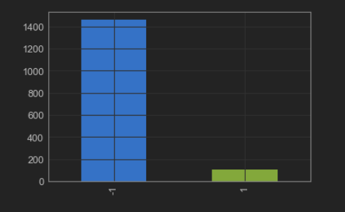
From Figure 1 it can be observed that the target variable is imbalanced and it is highly recommended to deal with this problem before the model building phase to avoid bias model. Xgboost is one of the models which can deal with imbalance classes but one needs to spend a lot of time to tune the hyper-parameters to achieve the best from the model.

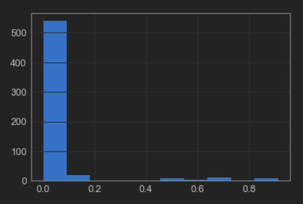
The dataset in hand contains a lot of null values and the next step would be to analyse these null values and remove the columns having null values more than a certain percentage. This percentage is calculated based on 95th quantile of null values.

#2. Analyzing nulls
secom_rmNa.isnull().sum().sum()
secom_nulls = secom_rmNa.isnull().sum()/len(secom_rmNa)
secom_nulls.describe()
secom_nulls.hist()

Figure 2: Missing percentge in each column

Now we calculate the 95th percentile of the null values.

x = secom_nulls.quantile(0.95)
secom_rmNa = secom_merged[secom_merged.columns[secom_nulls < x]]

Figure 3: Missing percentage after removing columns with more then 45% Na

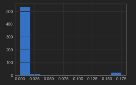
From figure 3 its visible that there are still missing values in the dataset and can be dealt by using many imputation methods. The most common method is to impute these values by mean, median or mode. There also exist few sophisticated techniques like K-nearest neighbour and interpolation.  We will be applying interpolation technique to our dataset. 

secom_complete = secom_rmNa.interpolate()

To prepare our dataset for analysis we should remove some more unwanted columns like columns with near zero variance. For this we can calulate number of unique values in each column and if there is only one unique value we can delete the column as it holds no information.

df = secom_complete.loc[:,secom_complete.apply(pd.Series.nunique) != 1]

## Let's check the shape of the df
df.shape
(1567, 444)

We have applied few data cleaning techniques and reduced the features from 590 to 444. However, In the next article we will apply some feature engineering techniques and adress problems like the curse of dimensionality and will also try to balance the target variable.

Bleiben Sie dran!!

Fuzzy Matching mit dem Jaro-Winkler-Score zur Auswertung von Markenbekanntheit und Werbeerinnerung

Für Unternehmen sind Markenbekanntheit und Werbeerinnerung wichtige Zielgrößen, denn anhand dieser lässt sich ableiten, ob Konsumenten ein Produkt einer Marke kaufen werden oder nicht. Zielgrößen wie diese werden von Marktforschungsinstituten über Befragungen ermittelt. Dafür wird in regelmäßigen Zeitabständen eine gleichbleibende Anzahl an Personen befragt, ob diese sich an Marken einer bestimmten Branche erinnern oder sich an Werbung erinnern. Die Personen füllen dafür in der Regel einen Onlinefragebogen aus.

Die Ergebnisse der Befragung liegen in einer Datenmatrix (siehe Tabelle) vor und müssen zur Auswertung zunächst bearbeitet werden.

Laufende Nummer Marke 1 Marke 2 Marke 3 Marke 4
1 ING-Diba Citigroup Sparkasse
2 Sparkasse Consorsbank
3 Commerbank Deutsche Bank Sparkasse ING-DiBa
4 Sparkasse Targobank

Ziel ist es aus diesen Daten folgende 0/1 codierte Matrix zu generieren. Wenn eine Marke bekannt ist, wird in die zur Marke gehörende Spalte eine Eins eingetragen, ansonsten eine Null.

Alle Marken ING-Diba Citigroup Sparkasse Targobank
ING-Diba, Citigroup, Sparkasse 1 1 1 0
Sparkasse, Consorsbank 0 0 1 0
Commerzbank, Deutsche Bank, Sparkasse, ING-Diba 1 0 0 0
Sparkasse, Targobank 0 0 1 1

Der Workflow um diese Datentransformation durchzuführen ist oftmals mittels eines Teilstrings einer Marke zu suchen ob diese in einem über alle Nennungen hinweg zusammengeführten String vorkommt oder nicht (z.B. „argo“ bei Targobank). Das Problem dieser Herangehensweise ist, dass viele falsch geschriebenen Wörter so nicht erfasst werden und die Erfahrung zeigt, dass falsch geschriebene Marken in vielfältigster Weise auftreten. Hier mussten in der Vergangenheit Mitarbeiter sich in stundenlangem Kampf durch die Ergebnisse wühlen und falsch zugeordnete oder nicht zugeordnete Marken händisch korrigieren und alle Variationen der Wörter notieren, um für die nächste Befragung das Suchpattern zu optimieren.

Eine Alternative diesen aufwändigen Workflow stellt die Ermittlung von falsch geschriebenen Wörtern mittels des Jaro-Winkler-Scores dar. Dafür muss zunächst die Jaro-Winkler-Distanz zwischen zwei Strings berechnet werden. Diese berechnet sich wie folgt:

d_j = \frac{1}{3}(\frac{m}{|s_1|}+\frac{m}{|s_2|}+\frac{m - t}{m})

  • m: Anzahl der übereinstimmenden Buchstaben
  • s: Länge des Strings
  • t: Hälfte der Anzahl der Umstellungen der Buchstaben die nötig sind, damit Strings identisch sind. („Ta“ und „gobank“ befinden sich bereits in der korrekten Reihenfolge, somit gilt: t = 0)

Aus dem Ergebnis lässt sich der Jaro-Winkler Score berechnen:
d_w = \d_j + (l_p (1 - d_j))
ist dabei die Jaro-Winkler-Distanz, l die Länge der übereinstimmenden Buchstaben von Beginn des Wortes bis zum maximal vierten Buchstaben und p ein konstanter Faktor von 0,1.

Für die Strings „Targobank“ und „Tangobank“ ergibt sich die Jaro-Winkler-Distanz:

d_j = \frac{1}{3}(\frac{8}{9}+\frac{8}{9}+\frac{8 - 0}{9})

Daraus wird im nächsten Schritt der Jaro-Winkler Score berechnet:

d_w = 0,9259 + (2 \cdot 0,1 (1 - 0,9259)) = 0,9407407

Bisherige Erfahrungen haben gezeigt, dass sich Scores ab 0,8 bzw. 0,9 am besten zur Suche von ähnlichen Wörtern eignen. Ein Schwellenwert darunter findet sehr viele Wörter, die sich z.B. auch anderen Wörtern zuordnen lassen. Ein Schwellenwert über 0,9 identifiziert falsch geschriebene Wörter oftmals nicht mehr.

Nach diesem theoretischen Exkurs möchte ich nun zeigen, wie sich das Ganze praktisch anwenden lässt. Da sich das Ganze um ein fiktives Beispiel handelt, werden zur Demonstration der Praxistauglichkeit Fakedaten mit folgendem Code erzeugt. Dabei wird angenommen, dass Personen unterschiedlich viele Banken kennen und diese mit einer bestimmten Wahrscheinlichkeit falsch schreiben.

# Erstellung von Fakeantworten
set.seed(1234)
library(stringi)
library(tidyr)
library(RecordLinkage)
library(xlsx)
library(tm)
library(qdap)
library(stringr)
library(openxlsx)

konsonant <- c("r", "n", "g", "h", "b")
vokal <- c("a", "e", "o", "i", "u")

# Funktion, die mit einer zu bestimmenden Wahrscheinlichkeit, einen zufälligen Buchstaben erzeugt.
generate_wrong_words <- function(x, p, k = TRUE) {
  if(runif(1, 0, 1) > p) { # Zufallswert zwischen 0 und 1
    if(k == TRUE) { # Konsonant oder Vokal erzeugen
      string <- konsonant[sample.int(5, 1)] # Zufallszahl, die Index des Konsonnanten-Vektors bestimmt.
    } else {
      string <- vokal[sample.int(5, 1)] # Zufallszahl, die Index eines Vokal-Vecktors bestimmt.
    }
  } else {
    string <- x
  }
  return(string)
}

randombank <- function(x) {
  random_num <- runif(1, 0, 1)
  if(random_num  > x) { ## Wahrscheinlichkeit, dass Person keine Bank kennt.
    number <- sample.int(7, 1)
    if(number == 1) {
      bank <- paste0("Ta", generate_wrong_words(x = "r", p = 0.7), "gob", generate_wrong_words(x = "a", p = 0.9), "nk")
    } else if (number == 2) {
      bank <- paste0("Ing-di", generate_wrong_words(x = "b", p = 0.6), "a")
    } else if (number == 3) {
      bank <- paste0("com", generate_wrong_words(x = "m", p = 0.7), "erzb", generate_wrong_words(x = "a", p = 0.8), "nk")
    } else if (number == 4){
      bank <- paste0("Deutsch", generate_wrong_words(x = "e", p = 0.6, k = FALSE), " Ban", generate_wrong_words(x = "k", p = 0.8))
    } else if (number == 5) {
      bank <- paste0("Spark", generate_wrong_words(x = "a", p = 0.7, k = FALSE), "sse")
    } else if (number == 6) {
      bank <- paste0("Cons", generate_wrong_words(x = "o", p = 0.7, k = FALSE), "rsbank")
    } else {
      bank <- paste0("Cit", generate_wrong_words(x = "i", p = 0.7, k = FALSE), "gro", generate_wrong_words(x = "u", p = 0.9, k = FALSE), "p")
    }
  } else {
    bank <- "" # Leerer String, wenn keine Bank bekannt.
  }
  return(bank)
}


# DataFrame erzeugen, in dem Werte gespeichert werden.
df_raw <- data.frame(matrix(ncol = 8, nrow = 2500))

# Erzeugen von richtig und falsch geschrieben Banken mit einer durch bestimmten Variabilität an Banken, welche die Personen kennen.
for(i in 1:2500) {
  df_raw [i, 1] <- i # Laufende Nummer des Befragten
  df_raw [i, 2] <- randombank(x = 0.05)
  if(df_raw [i, 2] == "") { df_raw [i, 3] <- "" } else {df_raw [i, 3] <- randombank(x = 0.1)}
  if(df_raw [i, 3] == "") { df_raw [i, 4] <- "" } else {df_raw [i, 4] <- randombank(x = 0.1)}
  if(df_raw [i, 4] == "") { df_raw [i, 5] <- "" } else {df_raw [i, 5] <- randombank(x = 0.15)} 
  if(df_raw [i, 5] == "") { df_raw [i, 6] <- "" } else {df_raw [i, 6] <- randombank(x = 0.15)}
  if(df_raw [i, 6] == "") { df_raw [i, 7] <- "" } else {df_raw [i, 7] <- randombank(x = 0.2)} 
  if(df_raw [i, 7] == "") { df_raw [i, 8] <- "" } else {df_raw [i, 8] <- randombank(x = 0.2)} 
}
colnames(df_raw)[1] <- "lfdn"

Ausführen:

head(df_raw)

Nun werden die Inhalte der Spalten in eine einzige Spalte zusammengefasst und jede Marke per Komma getrennt.

df <- unite(df_raw, united, c(2:ncol(df_raw)), sep = ",")
colnames(df)[2] <- "text"
# Gesuchte Banken (nur korrekt geschrieben)
startliste <- c("Targobank", "Ing-DiBa", "Commerzbank", "Deutsche Bank", "Sparkasse", "Consorsbank", "Citigroup")

Damit Sonderzeichen, Leerzeichen oder Groß- und Kleinschreibung keine Rolle spielen, werden alle Strings vereinheitlicht und störende Zeichen entfernt.

dftext <- tolower(dftext)
dftext <- str_trim(dftext)
dftext <- gsub(" ", "", dftext)
dftext <- gsub("[?]", "", dftext)
dftext <- gsub("[-]", "", dftext)
dftext <- gsub("[_]", "", dftext)

startliste <- tolower(startliste)
startliste <- str_trim(startliste)
startliste <- gsub(" ", "", startliste)
startliste <- gsub("[?]", "", startliste)
startliste <- gsub("[-]", "", startliste)
startliste <- gsub("[_]", "", startliste)

Im nächsten Schritt wird geprüft welche Schreibweisen überhaupt existieren. Dafür eignet sich eine Word-Frequency-Matrix, mit der alle einzigartigen Wörter und deren Häufigkeiten in einem Vektor gezählt wird.

words <- as.data.frame(wfm(dftext)) # Jedes einzigartige Wort und dazugehörige Häufigkeiten. words <- rownames(words) # wfm zählt Häufigkeiten jedes Wortes und schreibt Wörter in rownames, wir brauchen jedoch das Wort selbst. </pre> Danach wird eine leere Liste erstellt, in der iterativ für jedes Element des Suchvektors ein Charactervektor erzeugt wird, der Wörter enthält, die einen Jaro-Winker Score von 0,9 oder höher besitzen. <pre class="theme:github lang:r decode:true ">for(i in 1:length(startliste)) {   finalewortliste[[i]] <- words[which(jarowinkler(startliste[[i]], words) > 0.9)] } </pre> Jetzt wird ein leerer DataFrame erzeugt, der die Zeilenlänge des originalen DataFrames besitzt sowie die Anzahl der Marken als Spaltenlänge. <pre class="theme:github lang:r decode:true ">finaldf <- data.frame(matrix(nrow = nrow(df), ncol = length(startliste))) colnames(finaldf) <- startliste </pre> Im nächsten Schritt wird nun aus den ähnlichen Wörtern mit einer oder-Verknüpfung einen String erzeugt, der alle durch den Jaro-Winkler-Score identifizierten Wörter beinhaltet. Wenn ein Treffer gefunden wird, wird in der Suchspalte eine Eins eingetragen, ansonsten eine Null. <pre class="theme:github lang:r decode:true ">for(i in 1:ncol(finaldf)) {   finaldf[i] <- ifelse(str_detect(dftext, paste(finalewortliste[[i]], collapse = "|")) == TRUE, 1, 0) 
}

Zuletzt wird eine Spalte erzeugt, in die eine Eins geschrieben wird, wenn keine der Marken gefunden wurde.

finaldfkeinedergeannten <- ifelse(rowSums(finaldf) > 0, 0, 1) # Wenn nicht mindestens eine der gesuchten Banken bekannt </pre> Nach der fertigen Berechnung der Matrix können nun die finalen KPI´s berechnet und als Report in eine .xlsx Datei geschrieben werden. <pre class="theme:github lang:r decode:true "># Prozentuale Anteile berechnen. anteil <- as.data.frame(t(sapply(finaldf, sum) / nrow(finaldf) * 100)) # Ordne dem DataFrame die ursprünglichen Nenneungen zu. finaldf <- cbind(dftext, finaldf)
colnames(finaldf)[1] <- "text"

# Ergebnisse in eine .xlsx Datei schreiben.
wb <- createWorkbook()
addWorksheet(wb, "Ergebnisse")    
writeData(wb, "Ergebnisse", anteil, startCol = 2, startRow = 1, rowNames = FALSE)
writeData(wb, "Ergebnisse", finaldf, startCol = 1, startRow = 4, rowNames = FALSE)
saveWorkbook(wb, paste0("C:/Users/User/Desktop/Results_", Sys.Date(), ".xlsx"), overwrite = TRUE)  

Dieses Vorgehen kann natürlich nicht verhindern, dass sich jemand mit kritischem Auge die Daten anschauen muss. In mehreren Tests ergaben sich bei einer Fallzahl von ~10.000 Antworten Genauigkeiten zwischen 95% und 100%, was bisherige Ansätze um ein Vielfaches übertrifft.9407407

Big Data has reduced the boundary between demand-centric dynamic pricing and user-behavior centric pricing!

Real-time pricing is also known as Dynamic pricing, and it is a method to plan and set highly flexible prices of the services or the products. Dynamic pricing is aimed to help the online organizations modify the costs on the fly in relation to the ever changing market conditions. All sorts of modifications are managed the costing bots, who collect the information, and use the algorithms in order to regulate the costing, keeping in mind the set guidelines. With the help of data analysis, vendors can accurately forecast the best prices, and also can adjust it as per the changing needs.

What’s the role of Big Data in Dynamics pricing?

Big data strategies are made just to get the required insights which help to enhance the performance of a business. Still, companies find it difficult to understand the capabilities of analytics, and how the analytics can be used to make the process of pricing all the more powerful. Various levels of Big Data collection, and analysis result into planning a proper dynamics pricing structure. The Big Data captured by the companies hold a lot of value when it comes to devising solid, and very workable dynamics costing structures.

Each and every one of the data-oriented firms move from the basic data reporting stage via a plenty of stages to get to the utmost, desirable level of optimization that’s deemed the most sophisticated. This eventually helps to enhance the revenue management process as well.

How Big Data lessens the gap between demand-centric dynamic pricing and user-behavior centric pricing?

Big Data as we have discussed above has a major role to play when it comes to setting dynamic pricing plans. Dynamic pricing is now further categorized into different segments and two of them are demand-centric dynamic pricing and user-behavior centric pricing. Both of these hold equal importance in creating a top pricing strategy. However, one of the other important things is that, it acts as a liaison between the two as well.  It bridges the gap between the two. When it comes to demand centric costing, it is referred to as what the customer needs, and what the customer is looking for. Whereas, when it comes to user behavior pricing, it is more related to what we should be offering to the customer as per the interest levels of the customers.

Now, both of these parameters hold equal importance when it comes to making costing strategies that are fruitful. To set proper ‘demand centric pricing’ it is importance to know about the demand as well as the wants of the target audience. And, when it comes to user-behavior centric pricing, we need to know how the user is feeling, and what interest areas are. This where the role of Big Data analytics come into play.

Big Data analytics of relative information helps to find out both, the demands and well as the user behaviors. Big Data analytics done to study the target audience are a best way to get to the answers. Once we know about the demands and the user behavior we have to combine both of these to churn our better pricing strategies.

The costing plans should be taken into consideration by mapping both of these elements together. For example, even whenever we curate marketing strategies, they are basically catering to the demands of the public. But, at the same time, user-behavior is never neglected either. It’s a mix of both that we need for setting dynamic prices as well. The modifications which should be done in the pricing should be done based on collective insights gained by clubbing both the elements together.

By studying both the demands graphs as well as the user behavior reports, a company can devise plans that will turn out to be very useful when it comes to costing. Dynamic pricing is as it is a very fruitful invention, and the integration of Big Data has made it all the more powerful.

Big Data is one of those technologies which has made a lot possible in a lot of areas. Be it the pricing structures or the business strategies, Big Data analytics are used everywhere to improve the performance of the company.