Tag Archive for: R

Web Scraping Using R..!

In this blog, I’ll show you, How to Web Scrape using R..?

What is R..?

R is a programming language and its environment built for statistical analysis, graphical representation & reporting. R programming is mostly preferred by statisticians, data miners, and software programmers who want to develop statistical software.

R is also available as Free Software under the terms of the Free Software Foundation’s GNU General Public License in source code form.

Reasons to choose R

Reasons to choose R

Let’s begin our topic of Web Scraping using R.

Step 1- Select the website & the data you want to scrape.

I picked this website “https://www.alexa.com/topsites/countries/IN” and want to scrape data of Top 50 sites in India.

Data we want to scrape

Data we want to scrape

Step 2- Get to know the HTML tags using SelectorGadget.

In my previous blog, I already discussed how to inspect & find the proper HTML tags. So, now I’ll explain an easier way to get the HTML tags.

You have to go to Google chrome extension (chrome://extensions) & search SelectorGadget. Add it to your browser, it’s a quite good CSS selector.

Step 3- R Code

Evoking Important Libraries or Packages

I’m using RVEST package to scrape the data from the webpage; it is inspired by libraries like Beautiful Soup. If you didn’t install the package yet, then follow the code in the snippet below.

Step 4- Set the url of the website

Step 5- Find the HTML tags using SelectorGadget

It’s quite easy to find the proper HTML tags in which your data is present.

Firstly, I have to click on data using SelectorGadget which I want to scrape, it automatically selects the data which are similar to selected HTML tags. Before going forward, cross-check the selected values, are they correct or some junk data is also gets selected..? If you noticed our page has only 50 values, but you can see 156 values are selected.

Selection by SelectorGadget

Selection by SelectorGadget

So I need to remove unwanted values who get selected, once you click on them to deselect it, it turns red and others will turn yellow except our primary selection which turn to green. Now you can see only 50 values are selected as per our primary requirement but it’s not enough. I have to again cross-check that some required values are not exchanged with junk values.

If we satisfy with our selection then copy the HTML tag & include it into the code, else repeat this exercise.

Modified Selection by SelectorGadget

Step 6- Include the tag in our Code

After including the tags, our code is like this.

Code Snippet

If I run the code, values in each list object will be 50.

Data Stored in List Objects

Step 7- Creating DataFrame

Now, we create a dataframe with our list-objects. So for creating a dataframe, we always need to remember one thumb rule that is the number of rows (length of all the lists) should be equal, else we get an error.

Error appears when number of rows differs

Finally, Our DataFrame will look like this:

Our Final Data

Step 8- Writing our DataFrame to CSV file

We need our scraped data to be available locally for further analysis & model building or other purposes.

Our final piece of code to write it in CSV file is:

Writing to CSV file

Step 9- Check the CSV file

Data written in CSV file

Conclusion-

I tried to explain Web Scraping using R in a simple way, Hope this will help you in understanding it better.

Find full code on

https://github.com/vgyaan/Alexa/blob/master/webscrap.R

If you have any questions about the code or web scraping in general, reach out to me on LinkedIn!

Okay, we will meet again with the new exposer.

Till then,

Happy Coding..!

Python vs R: Which Language to Choose for Deep Learning?

Data science is increasingly becoming essential for every business to operate efficiently in this modern world. This influences the processes composed together to obtain the required outputs for clients. While machine learning and deep learning sit at the core of data science, the concepts of deep learning become essential to understand as it can help increase the accuracy of final outputs. And when it comes to data science, R and Python are the most popular programming languages used to instruct the machines.

Python and R: Primary Languages Used for Deep Learning

Deep learning and machine learning differentiate based on the input data type they use. While machine learning depends upon the structured data, deep learning uses neural networks to store and process the data during the learning. Deep learning can be described as the subset of machine learning, where the data to be processed is defined in another structure than a normal one.

R is developed specifically to support the concepts and implementation of data science and hence, the support provided by this language is incredible as writing codes become much easier with its simple syntax.

Python is already much popular programming language that can serve more than one development niche without straining even for a bit. The implementation of Python for programming machine learning algorithms is very much popular and the results provided are accurate and faster than any other language. (C or Java). And because of its extended support for data science concept implementation, it becomes a tough competitor for R.

However, if we compare the charts of popularity, Python is obviously more popular among data scientists and developers because of its versatility and easier usage during algorithm implementation. However, R outruns Python when it comes to the packages offered to developers specifically expertise in R over Python. Therefore, to conclude which one of them is the best, let’s take an overview of the features and limits offered by both languages.

Python

Python was first introduced by Guido Van Rossum who developed it as the successor of ABC programming language. Python puts white space at the center while increasing the readability of the developed code. It is a general-purpose programming language that simply extends support for various development needs.

The packages of Python includes support for web development, software development, GUI (Graphical User Interface) development and machine learning also. Using these packages and putting the best development skills forward, excellent solutions can be developed. According to Stackoverflow, Python ranks at the fourth position as the most popular programming language among developers.

Benefits for performing enhanced deep learning using Python are:

  • Concise and Readable Code
  • Extended Support from Large Community of Developers
  • Open-source Programming Language
  • Encourages Collaborative Coding
  • Suitable for small and large-scale products

The latest and stable version of Python has been released as Python 3.8.0 on 14th October 2019. Developing a software solution using Python becomes much easier as the extended support offered through the packages drives better development and answers every need.

R

R is a language specifically used for the development of statistical software and for statistical data analysis. The primary user base of R contains statisticians and data scientists who are analyzing data. Supported by R Foundation for statistical computing, this language is not suitable for the development of websites or applications. R is also an open-source environment that can be used for mining excessive and large amounts of data.

R programming language focuses on the output generation but not the speed. The execution speed of programs written in R is comparatively lesser as producing required outputs is the aim not the speed of the process. To use R in any development or mining tasks, it is required to install its operating system specific binary version before coding to run the program directly into the command line.

R also has its own development environment designed and named RStudio. R also involves several libraries that help in crafting efficient programs to execute mining tasks on the provided data.

The benefits offered by R are pretty common and similar to what Python has to offer:

  • Open-source programming language
  • Supports all operating systems
  • Supports extensions
  • R can be integrated with many of the languages
  • Extended Support for Visual Data Mining

Although R ranks at the 17th position in Stackoverflow’s most popular programming language list, the support offered by this language has no match. After all, the R language is developed by statisticians for statisticians!

Python vs R: Should They be Really Compared?

Even when provided with the best technical support and efficient tools, a developer will not be able to provide quality outputs if he/she doesn’t possess the required skills. The point here is, technical skills rank higher than the resources provided. A comparison of these two programming languages is not advisable as they both hold their own set of advantages. However, the developers considering to use both together are less but they obtain maximum benefit from the process.

Both these languages have some features in common. For example, if a representative comes asking you if you lend technical support for developing an uber clone, you are directly going to decline as Python and R both do not support mobile app development. To benefit the most and develop excellent solutions using both these programming languages, it is advisable to stop comparing and start collaborating!

R and Python: How to Fit Both In a Single Program

Anticipating the future needs of the development industry, there has been a significant development to combine these both excellent programming languages into one. Now, there are two approaches to performing this: either we include R script into Python code or vice versa.

Using the available interfaces, packages and extended support from Python we can include R script into the code and enhance the productivity of Python code. Availability of PypeR, pyRserve and more resources helps run these two programming languages efficiently while efficiently performing the background work.

Either way, using the developed functions and packages made available for integrating Python in R are also effective at providing better results. Available R packages like rJython, rPython, reticulate, PythonInR and more, integrating Python into R language is very easy.

Therefore, using the development skills at their best and maximizing the use of such amazing resources, Python and R can be togetherly used to enhance end results and provide accurate deep learning support.

Conclusion

Python and R both are great in their own names and own places. However, because of the wide applications of Python in almost every operation, the annual packages offered to Python developers are less than the developers skilled in using R. However, this doesn’t justify the usability of R. The ultimate decision of choosing between these two languages depends upon the data scientists or developers and their mining requirements.

And if a developer or data scientist decides to develop skills for both- Python and R-based development, it turns out to be beneficial in the near future. Choosing any one or both to use in your project depends on the project requirements and expert support on hand.

Multi-touch attribution: A data-driven approach

Customers shopping behavior has changed drastically when it comes to online shopping, as nowadays, customer likes to do a thorough market research about a product before making a purchase.

What is Multi-touch attribution?

This makes it really hard for marketers to correctly determine the contribution for each marketing channel to which a customer was exposed to. The path a customer takes from his first search to the purchase is known as a Customer Journey and this path consists of multiple marketing channels or touchpoints. Therefore, it is highly important to distribute the budget between these channels to maximize return. This problem is known as multi-touch attribution problem and the right attribution model helps to steer the marketing budget efficiently. Multi-touch attribution problem is well known among marketers. You might be thinking that if this is a well known problem then there must be an algorithm out there to deal with this. Well, there are some traditional models  but every model has its own limitation which will be discussed in the next section.

Types of attribution models

Most of the eCommerce companies have a performance marketing department to make sure that the marketing budget is spent in an agile way. There are multiple heuristics attribution models pre-existing in google analytics however there are several issues with each one of them. These models are:

Traditional attribution models

First touch attribution model

100% credit is given to the first channel as it is considered that the first marketing channel was responsible for the purchase.

Figure 1: First touch attribution model

Last touch attribution model

100% credit is given to the last channel as it is considered that the first marketing channel was responsible for the purchase.

Figure 2: Last touch attribution model

Linear-touch attribution model

In this attribution model, equal credit is given to all the marketing channels present in customer journey as it is considered that each channel is equally responsible for the purchase.

Figure 3: Linear attribution model

U-shaped or Bath tub attribution model

This is most common in eCommerce companies, this model assigns 40% to first and last touch and 20% is equally distributed among the rest.

Figure 4: Bathtub or U-shape attribution model

Data driven attribution models

Traditional attribution models follows somewhat a naive approach to assign credit to one or all the marketing channels involved. As it is not so easy for all the companies to take one of these models and implement it. There are a lot of challenges that comes with multi-touch attribution problem like customer journey duration, overestimation of branded channels, vouchers and cross-platform issue, etc.

Switching from traditional models to data-driven models gives us more flexibility and more insights as the major part here is defining some rules to prepare the data that fits your business. These rules can be defined by performing an ad hoc analysis of customer journeys. In the next section, I will discuss about Markov chain concept as an attribution model.

Markov chains

Markov chains concepts revolves around probability. For attribution problem, every customer journey can be seen as a chain(set of marketing channels) which will compute a markov graph as illustrated in figure 5. Every channel here is represented as a vertex and the edges represent the probability of hopping from one channel to another. There will be an another detailed article, explaining the concept behind different data-driven attribution models and how to apply them.

Figure 5: Markov chain example

Challenges during the Implementation

Transitioning from a traditional attribution models to a data-driven one, may sound exciting but the implementation is rather challenging as there are several issues which can not be resolved just by changing the type of model. Before its implementation, the marketers should perform a customer journey analysis to gain some insights about their customers and try to find out/perform:

  1. Length of customer journey.
  2. On an average how many branded and non branded channels (distinct and non-distinct) in a typical customer journey?
  3. Identify most upper funnel and lower funnel channels.
  4. Voucher analysis: within branded and non-branded channels.

When you are done with the analysis and able to answer all of the above questions, the next step would be to define some rules in order to handle the user data according to your business needs. Some of the issues during the implementation are discussed below along with their solution.

Customer journey duration

Assuming that you are a retailer, let’s try to understand this issue with an example. In May 2016, your company started a Fb advertising campaign for a particular product category which “attracted” a lot of customers including Chris. He saw your Fb ad while working in the office and clicked on it, which took him to your website. As soon as he registered on your website, his boss called him (probably because he was on Fb while working), he closed everything and went for the meeting. After coming back, he started working and completely forgot about your ad or products. After a few days, he received an email with some offers of your products which also he ignored until he saw an ad again on TV in Jan 2019 (after 3 years). At this moment, he started doing his research about your products and finally bought one of your products from some Instagram campaign. It took Chris almost 3 years to make his first purchase.

Figure 6: Chris journey

Now, take a minute and think, if you analyse the entire journey of customers like Chris, you would realize that you are still assigning some of the credit to the touchpoints that happened 3 years ago. This can be solved by using an attribution window. Figure 6 illustrates that 83% of the customers are making a purchase within 30 days which means the attribution window here could be 30 days. In simple words, it is safe to remove the touchpoints that happens after 30 days of purchase. This parameter can also be changed to 45 days or 60 days, depending on the use case.

Figure 7: Length of customer journey

Removal of direct marketing channel

A well known issue that every marketing analyst is aware of is, customers who are already aware of the brand usually comes to the website directly. This leads to overestimation of direct channel and branded channels start getting more credit. In this case, you can set a threshold (say 7 days) and remove these branded channels from customer journey.

Figure 8: Removal of branded channels

Cross platform problem

If some of your customers are using different devices to explore your products and you are not able to track them then it will make retargeting really difficult. In a perfect world these customers belong to same journey and if these can’t be combined then, except one, other paths would be considered as “non-converting path”. For attribution problem device could be thought of as a touchpoint to include in the path but to be able to track these customers across all devices would still be challenging. A brief introduction to deterministic and probabilistic ways of cross device tracking can be found here.

Figure 9: Cross platform clash

How to account for Vouchers?

To better account for vouchers, it can be added as a ‘dummy’ touchpoint of the type of voucher (CRM,Social media, Affiliate or Pricing etc.) used. In our case, we tried to add these vouchers as first touchpoint and also as a last touchpoint but no significant difference was found. Also, if the marketing channel of which the voucher was used was already in the path, the dummy touchpoint was not added.

Figure 10: Addition of Voucher as a touchpoint

Fuzzy Matching mit dem Jaro-Winkler-Score zur Auswertung von Markenbekanntheit und Werbeerinnerung

Für Unternehmen sind Markenbekanntheit und Werbeerinnerung wichtige Zielgrößen, denn anhand dieser lässt sich ableiten, ob Konsumenten ein Produkt einer Marke kaufen werden oder nicht. Zielgrößen wie diese werden von Marktforschungsinstituten über Befragungen ermittelt. Dafür wird in regelmäßigen Zeitabständen eine gleichbleibende Anzahl an Personen befragt, ob diese sich an Marken einer bestimmten Branche erinnern oder sich an Werbung erinnern. Die Personen füllen dafür in der Regel einen Onlinefragebogen aus.

Die Ergebnisse der Befragung liegen in einer Datenmatrix (siehe Tabelle) vor und müssen zur Auswertung zunächst bearbeitet werden.

Laufende Nummer Marke 1 Marke 2 Marke 3 Marke 4
1 ING-Diba Citigroup Sparkasse
2 Sparkasse Consorsbank
3 Commerbank Deutsche Bank Sparkasse ING-DiBa
4 Sparkasse Targobank

Ziel ist es aus diesen Daten folgende 0/1 codierte Matrix zu generieren. Wenn eine Marke bekannt ist, wird in die zur Marke gehörende Spalte eine Eins eingetragen, ansonsten eine Null.

Alle Marken ING-Diba Citigroup Sparkasse Targobank
ING-Diba, Citigroup, Sparkasse 1 1 1 0
Sparkasse, Consorsbank 0 0 1 0
Commerzbank, Deutsche Bank, Sparkasse, ING-Diba 1 0 0 0
Sparkasse, Targobank 0 0 1 1

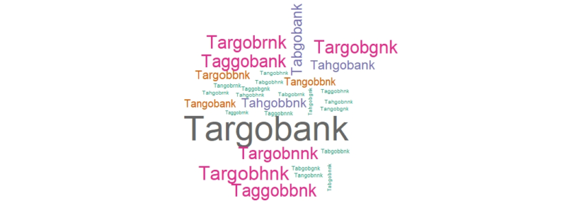
Der Workflow um diese Datentransformation durchzuführen ist oftmals mittels eines Teilstrings einer Marke zu suchen ob diese in einem über alle Nennungen hinweg zusammengeführten String vorkommt oder nicht (z.B. „argo“ bei Targobank). Das Problem dieser Herangehensweise ist, dass viele falsch geschriebenen Wörter so nicht erfasst werden und die Erfahrung zeigt, dass falsch geschriebene Marken in vielfältigster Weise auftreten. Hier mussten in der Vergangenheit Mitarbeiter sich in stundenlangem Kampf durch die Ergebnisse wühlen und falsch zugeordnete oder nicht zugeordnete Marken händisch korrigieren und alle Variationen der Wörter notieren, um für die nächste Befragung das Suchpattern zu optimieren.

Eine Alternative diesen aufwändigen Workflow stellt die Ermittlung von falsch geschriebenen Wörtern mittels des Jaro-Winkler-Scores dar. Dafür muss zunächst die Jaro-Winkler-Distanz zwischen zwei Strings berechnet werden. Diese berechnet sich wie folgt:

d_j = \frac{1}{3}(\frac{m}{|s_1|}+\frac{m}{|s_2|}+\frac{m - t}{m})

  • m: Anzahl der übereinstimmenden Buchstaben
  • s: Länge des Strings
  • t: Hälfte der Anzahl der Umstellungen der Buchstaben die nötig sind, damit Strings identisch sind. („Ta“ und „gobank“ befinden sich bereits in der korrekten Reihenfolge, somit gilt: t = 0)

Aus dem Ergebnis lässt sich der Jaro-Winkler Score berechnen:
d_w = \d_j + (l_p (1 - d_j))
ist dabei die Jaro-Winkler-Distanz, l die Länge der übereinstimmenden Buchstaben von Beginn des Wortes bis zum maximal vierten Buchstaben und p ein konstanter Faktor von 0,1.

Für die Strings „Targobank“ und „Tangobank“ ergibt sich die Jaro-Winkler-Distanz:

d_j = \frac{1}{3}(\frac{8}{9}+\frac{8}{9}+\frac{8 - 0}{9})

Daraus wird im nächsten Schritt der Jaro-Winkler Score berechnet:

d_w = 0,9259 + (2 \cdot 0,1 (1 - 0,9259)) = 0,9407407

Bisherige Erfahrungen haben gezeigt, dass sich Scores ab 0,8 bzw. 0,9 am besten zur Suche von ähnlichen Wörtern eignen. Ein Schwellenwert darunter findet sehr viele Wörter, die sich z.B. auch anderen Wörtern zuordnen lassen. Ein Schwellenwert über 0,9 identifiziert falsch geschriebene Wörter oftmals nicht mehr.

Nach diesem theoretischen Exkurs möchte ich nun zeigen, wie sich das Ganze praktisch anwenden lässt. Da sich das Ganze um ein fiktives Beispiel handelt, werden zur Demonstration der Praxistauglichkeit Fakedaten mit folgendem Code erzeugt. Dabei wird angenommen, dass Personen unterschiedlich viele Banken kennen und diese mit einer bestimmten Wahrscheinlichkeit falsch schreiben.

# Erstellung von Fakeantworten
set.seed(1234)
library(stringi)
library(tidyr)
library(RecordLinkage)
library(xlsx)
library(tm)
library(qdap)
library(stringr)
library(openxlsx)

konsonant <- c("r", "n", "g", "h", "b")
vokal <- c("a", "e", "o", "i", "u")

# Funktion, die mit einer zu bestimmenden Wahrscheinlichkeit, einen zufälligen Buchstaben erzeugt.
generate_wrong_words <- function(x, p, k = TRUE) {
  if(runif(1, 0, 1) > p) { # Zufallswert zwischen 0 und 1
    if(k == TRUE) { # Konsonant oder Vokal erzeugen
      string <- konsonant[sample.int(5, 1)] # Zufallszahl, die Index des Konsonnanten-Vektors bestimmt.
    } else {
      string <- vokal[sample.int(5, 1)] # Zufallszahl, die Index eines Vokal-Vecktors bestimmt.
    }
  } else {
    string <- x
  }
  return(string)
}

randombank <- function(x) {
  random_num <- runif(1, 0, 1)
  if(random_num  > x) { ## Wahrscheinlichkeit, dass Person keine Bank kennt.
    number <- sample.int(7, 1)
    if(number == 1) {
      bank <- paste0("Ta", generate_wrong_words(x = "r", p = 0.7), "gob", generate_wrong_words(x = "a", p = 0.9), "nk")
    } else if (number == 2) {
      bank <- paste0("Ing-di", generate_wrong_words(x = "b", p = 0.6), "a")
    } else if (number == 3) {
      bank <- paste0("com", generate_wrong_words(x = "m", p = 0.7), "erzb", generate_wrong_words(x = "a", p = 0.8), "nk")
    } else if (number == 4){
      bank <- paste0("Deutsch", generate_wrong_words(x = "e", p = 0.6, k = FALSE), " Ban", generate_wrong_words(x = "k", p = 0.8))
    } else if (number == 5) {
      bank <- paste0("Spark", generate_wrong_words(x = "a", p = 0.7, k = FALSE), "sse")
    } else if (number == 6) {
      bank <- paste0("Cons", generate_wrong_words(x = "o", p = 0.7, k = FALSE), "rsbank")
    } else {
      bank <- paste0("Cit", generate_wrong_words(x = "i", p = 0.7, k = FALSE), "gro", generate_wrong_words(x = "u", p = 0.9, k = FALSE), "p")
    }
  } else {
    bank <- "" # Leerer String, wenn keine Bank bekannt.
  }
  return(bank)
}


# DataFrame erzeugen, in dem Werte gespeichert werden.
df_raw <- data.frame(matrix(ncol = 8, nrow = 2500))

# Erzeugen von richtig und falsch geschrieben Banken mit einer durch bestimmten Variabilität an Banken, welche die Personen kennen.
for(i in 1:2500) {
  df_raw [i, 1] <- i # Laufende Nummer des Befragten
  df_raw [i, 2] <- randombank(x = 0.05)
  if(df_raw [i, 2] == "") { df_raw [i, 3] <- "" } else {df_raw [i, 3] <- randombank(x = 0.1)}
  if(df_raw [i, 3] == "") { df_raw [i, 4] <- "" } else {df_raw [i, 4] <- randombank(x = 0.1)}
  if(df_raw [i, 4] == "") { df_raw [i, 5] <- "" } else {df_raw [i, 5] <- randombank(x = 0.15)} 
  if(df_raw [i, 5] == "") { df_raw [i, 6] <- "" } else {df_raw [i, 6] <- randombank(x = 0.15)}
  if(df_raw [i, 6] == "") { df_raw [i, 7] <- "" } else {df_raw [i, 7] <- randombank(x = 0.2)} 
  if(df_raw [i, 7] == "") { df_raw [i, 8] <- "" } else {df_raw [i, 8] <- randombank(x = 0.2)} 
}
colnames(df_raw)[1] <- "lfdn"

Ausführen:

head(df_raw)

Nun werden die Inhalte der Spalten in eine einzige Spalte zusammengefasst und jede Marke per Komma getrennt.

df <- unite(df_raw, united, c(2:ncol(df_raw)), sep = ",")
colnames(df)[2] <- "text"
# Gesuchte Banken (nur korrekt geschrieben)
startliste <- c("Targobank", "Ing-DiBa", "Commerzbank", "Deutsche Bank", "Sparkasse", "Consorsbank", "Citigroup")

Damit Sonderzeichen, Leerzeichen oder Groß- und Kleinschreibung keine Rolle spielen, werden alle Strings vereinheitlicht und störende Zeichen entfernt.

dftext <- tolower(dftext)
dftext <- str_trim(dftext)
dftext <- gsub(" ", "", dftext)
dftext <- gsub("[?]", "", dftext)
dftext <- gsub("[-]", "", dftext)
dftext <- gsub("[_]", "", dftext)

startliste <- tolower(startliste)
startliste <- str_trim(startliste)
startliste <- gsub(" ", "", startliste)
startliste <- gsub("[?]", "", startliste)
startliste <- gsub("[-]", "", startliste)
startliste <- gsub("[_]", "", startliste)

Im nächsten Schritt wird geprüft welche Schreibweisen überhaupt existieren. Dafür eignet sich eine Word-Frequency-Matrix, mit der alle einzigartigen Wörter und deren Häufigkeiten in einem Vektor gezählt wird.

words <- as.data.frame(wfm(dftext)) # Jedes einzigartige Wort und dazugehörige Häufigkeiten. words <- rownames(words) # wfm zählt Häufigkeiten jedes Wortes und schreibt Wörter in rownames, wir brauchen jedoch das Wort selbst. </pre> Danach wird eine leere Liste erstellt, in der iterativ für jedes Element des Suchvektors ein Charactervektor erzeugt wird, der Wörter enthält, die einen Jaro-Winker Score von 0,9 oder höher besitzen. <pre class="theme:github lang:r decode:true ">for(i in 1:length(startliste)) {   finalewortliste[[i]] <- words[which(jarowinkler(startliste[[i]], words) > 0.9)] } </pre> Jetzt wird ein leerer DataFrame erzeugt, der die Zeilenlänge des originalen DataFrames besitzt sowie die Anzahl der Marken als Spaltenlänge. <pre class="theme:github lang:r decode:true ">finaldf <- data.frame(matrix(nrow = nrow(df), ncol = length(startliste))) colnames(finaldf) <- startliste </pre> Im nächsten Schritt wird nun aus den ähnlichen Wörtern mit einer oder-Verknüpfung einen String erzeugt, der alle durch den Jaro-Winkler-Score identifizierten Wörter beinhaltet. Wenn ein Treffer gefunden wird, wird in der Suchspalte eine Eins eingetragen, ansonsten eine Null. <pre class="theme:github lang:r decode:true ">for(i in 1:ncol(finaldf)) {   finaldf[i] <- ifelse(str_detect(dftext, paste(finalewortliste[[i]], collapse = "|")) == TRUE, 1, 0) 
}

Zuletzt wird eine Spalte erzeugt, in die eine Eins geschrieben wird, wenn keine der Marken gefunden wurde.

finaldfkeinedergeannten <- ifelse(rowSums(finaldf) > 0, 0, 1) # Wenn nicht mindestens eine der gesuchten Banken bekannt </pre> Nach der fertigen Berechnung der Matrix können nun die finalen KPI´s berechnet und als Report in eine .xlsx Datei geschrieben werden. <pre class="theme:github lang:r decode:true "># Prozentuale Anteile berechnen. anteil <- as.data.frame(t(sapply(finaldf, sum) / nrow(finaldf) * 100)) # Ordne dem DataFrame die ursprünglichen Nenneungen zu. finaldf <- cbind(dftext, finaldf)
colnames(finaldf)[1] <- "text"

# Ergebnisse in eine .xlsx Datei schreiben.
wb <- createWorkbook()
addWorksheet(wb, "Ergebnisse")    
writeData(wb, "Ergebnisse", anteil, startCol = 2, startRow = 1, rowNames = FALSE)
writeData(wb, "Ergebnisse", finaldf, startCol = 1, startRow = 4, rowNames = FALSE)
saveWorkbook(wb, paste0("C:/Users/User/Desktop/Results_", Sys.Date(), ".xlsx"), overwrite = TRUE)  

Dieses Vorgehen kann natürlich nicht verhindern, dass sich jemand mit kritischem Auge die Daten anschauen muss. In mehreren Tests ergaben sich bei einer Fallzahl von ~10.000 Antworten Genauigkeiten zwischen 95% und 100%, was bisherige Ansätze um ein Vielfaches übertrifft.9407407

How To Remotely Send R and Python Execution to SQL Server from Jupyter Notebooks

Introduction

Did you know that you can execute R and Python code remotely in SQL Server from Jupyter Notebooks or any IDE? Machine Learning Services in SQL Server eliminates the need to move data around. Instead of transferring large and sensitive data over the network or losing accuracy on ML training with sample csv files, you can have your R/Python code execute within your database. You can work in Jupyter Notebooks, RStudio, PyCharm, VSCode, Visual Studio, wherever you want, and then send function execution to SQL Server bringing intelligence to where your data lives.

This tutorial will show you an example of how you can send your python code from Juptyter notebooks to execute within SQL Server. The same principles apply to R and any other IDE as well. If you prefer to learn through videos, this tutorial is also published on YouTube here:


Environment Setup Prerequisites

  1. Install ML Services on SQL Server

In order for R or Python to execute within SQL, you first need the Machine Learning Services feature installed and configured. See this how-to guide.

  1. Install RevoscalePy via Microsoft’s Python Client

In order to send Python execution to SQL from Jupyter Notebooks, you need to use Microsoft’s RevoscalePy package. To get RevoscalePy, download and install Microsoft’s ML Services Python Client. Documentation Page or Direct Download Link (for Windows).

After downloading, open powershell as an administrator and navigate to the download folder. Start the installation with this command (feel free to customize the install folder): .\Install-PyForMLS.ps1 -InstallFolder “C:\Program Files\MicrosoftPythonClient”

Be patient while the installation can take a little while. Once installed navigate to the new path you installed in. Let’s make an empty folder and open Jupyter Notebooks: mkdir JupyterNotebooks; cd JupyterNotebooks; ..\Scripts\jupyter-notebook

Create a new notebook with the Python 3 interpreter:


To test if everything is setup, import revoscalepy in the first cell and execute. If there are no error messages you are ready to move forward.

Database Setup (Required for this tutorial only)

For the rest of the tutorial you can clone this Jupyter Notebook from Github if you don’t want to copy paste all of the code. This database setup is a one time step to ensure you have the same data as this tutorial. You don’t need to perform any of these setup steps to use your own data.

  1. Create a database

Modify the connection string for your server and use pyodbc to create a new database.

import pyodbc  
# creating a new db to load Iris sample in 
new_db_name = "MLRemoteExec" connection_string = "Driver=SQL Server;Server=localhost\MSSQLSERVER2017;Database={0};Trusted_Connection=Yes;" 

cnxn = pyodbc.connect(connection_string.format("master"), autocommit=True) 

cnxn.cursor().execute("IF EXISTS(SELECT * FROM sys.databases WHERE [name] = '{0}') DROP DATABASE {0}".format(new_db_name)) 

cnxn.cursor().execute("CREATE DATABASE " + new_db_name)

cnxn.close()

print("Database created") 
  1. Import Iris sample from SkLearn

Iris is a popular dataset for beginner data science tutorials. It is included by default in sklearn package.

from sklearn import datasetsimport pandas as pd
# SkLearn has the Iris sample dataset built in to the packageiris = datasets.load_iris()
df = pd.DataFrame(iris.data, columns=iris.feature_names)
  1. Use RecoscalePy APIs to create a table and load the Iris data

(You can also do this with pyodbc, sqlalchemy or other packages)

from revoscalepy import RxSqlServerData, rx_data_step
# Example of using RX APIs to load data into SQL table. You can also do this with pyodbc
table_ref = RxSqlServerData(connection_string=connection_string.format(new_db_name), table="Iris")rx_data_step(input_data = df, output_file = table_ref, overwrite = True)print("New Table Created: Iris")
print("Sklearn Iris sample loaded into Iris table")

Define a Function to Send to SQL Server

Write any python code you want to execute in SQL. In this example we are creating a scatter matrix on the iris dataset and only returning the bytestream of the .png back to Jupyter Notebooks to render on our client.

def send_this_func_to_sql():
    from revoscalepy import RxSqlServerData, rx_import
    from pandas.tools.plotting import scatter_matrix
    import matplotlib.pyplot as plt
    import io    
# remember the scope of the variables in this func are within our SQL Server Python Runtime
    connection_string = "Driver=SQL Server;Server=localhost\MSSQLSERVER2017; Database=MLRemoteExec;Trusted_Connection=Yes;"

# specify a query and load into pandas dataframe df
    sql_query = RxSqlServerData(connection_string=connection_string, sql_query = "select * from Iris")

    df = rx_import(sql_query)
    scatter_matrix(df)

# return bytestream of image created by scatter_matrix
    buf = io.BytesIO()
    plt.savefig(buf, format="png")
    buf.seek(0)
    return buf.getvalue()

Send execution to SQL

Now that we are finally set up, check out how easy sending remote execution really is! First, import revoscalepy. Create a sql_compute_context, and then send the execution of any function seamlessly to SQL Server with RxExec. No raw data had to be transferred from SQL to the Jupyter Notebook. All computation happened within the database and only the image file was returned to be displayed.

from IPython import display
import matplotlib.pyplot as plt 
from revoscalepy import RxInSqlServer, rx_exec# create a remote compute context with connection to SQL Server

sql_compute_context = RxInSqlServer(connection_string=connection_string.format(new_db_name))

# use rx_exec to send the function execution to SQL Server

image = rx_exec(send_this_func_to_sql, compute_context=sql_compute_context)[0]

# only an image was returned to my jupyter client. All data remained secure and was manipulated in my db.

display.Image(data=image)

While this example is trivial with the Iris dataset, imagine the additional scale, performance, and security capabilities that you now unlocked. You can use any of the latest open source R/Python packages to build Deep Learning and AI applications on large amounts of data in SQL Server. We also offer leading edge, high-performance algorithms in Microsoft’s RevoScaleR and RevoScalePy APIs. Using these with the latest innovations in the open source world allows you to bring unparalleled selection, performance, and scale to your applications.

Learn More

Check out SQL Machine Learning Services Documentation to learn how you can easily deploy your R/Python code with SQL stored procedures making them accessible in your ETL processes or to any application. Train and store machine learning models in your database bringing intelligence to where your data lives.

Other YouTube Tutorials: