Data Dimensionality Reduction Series: Random Forest
Hello lovely individuals, I hope everyone is doing well, is fantastic, and is smiling more than usual. In this blog we shall discuss a very interesting term used to build many models in the Data science industry as well as the cyber security industry.
SUPER BASIC DEFINITION OF RANDOM FOREST:
Random forest is a form of Supervised Machine Learning Algorithm that operates on the majority rule. For example, if we have a number of different algorithms working on the same issue but producing different answers, the majority of the findings are taken into account. Random forests, also known as random selection forests, are an ensemble learning approach for classification, regression, and other problems that works by generating a jumble of decision trees during training.
When it comes to regression and classification, random forest can handle both categorical and continuous variable data sets. It typically helps us outperform other algorithms and overcome challenges like overfitting and the curse of dimensionality.
QUICK ANALOGY TO UNDERSTAND THINGS BETTER:
Uncle John wants to see a doctor for his acute abdominal discomfort, so he goes to his pals for recommendations on the top doctors in town. After consulting with a number of friends and family members, Atlas chooses to visit the doctor who received the highest recommendations.
So, what does this mean? The same is true for random forests. It builds decision trees from several samples and utilises their majority vote for classification and average for regression.
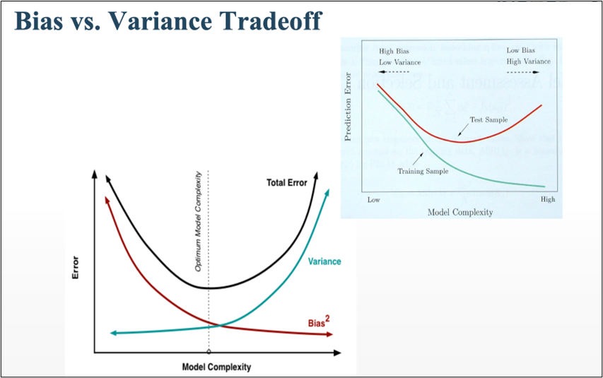
HOW BIAS AND VARIANCE AFFECTS THE ALGORITHM?
- BIAS
- The algorithm’s accuracy or quality is measured.
- High bias means a poor match
- VARIANCE
- The accuracy or specificity of the match is measured.
- A high variance means a weak match
We would like to minimise each of these. But, unfortunately we can’t do this independently, since there is a trade-off
EXPECTED PREDICTION ERROR = VARIANCE + BIAS^2 + NOISE^2
HOW IS IT DIFFERENT FROM OTHER TWO ALGORITHMS?
Every other data dimensionality reduction method, such as missing value ratio and principal component analysis, must be built from the scratch, but the best thing about random forest is that it comes with built-in features and is a tree-based model that uses a combination of decision trees for non-linear data classification and regression.
Without wasting much time, let’s move to the main part where we’ll discuss the working of RANDOM FOREST:
WORKING WITH RANDOM FOREST:
As we saw in the analogy, RANDOM FOREST operates on the basis of ensemble technique; however, what precisely does ensemble technique mean? It’s actually rather straightforward. Ensemble simply refers to the combination of numerous models. As a result, rather than a single model, a group of models is utilised to create predictions.
ENSEMBLE TECHNIQUE HAS 2 METHODS:
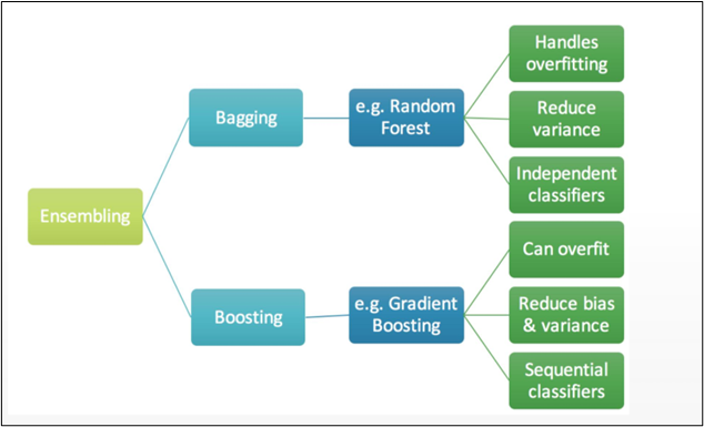
1] BAGGING
2] BOOSTING

Let’s dive deep to understand things better:
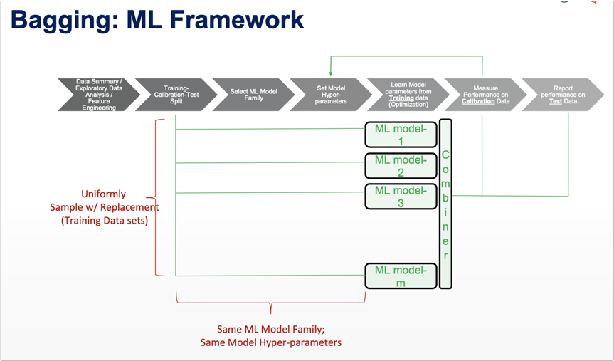
1] BAGGING:
LET’S UNDERSTAND IT THROUGH A BETTER VIEW:

Bagging simply helps us to reduce the variance in a loud datasets. It works on an ensemble technique.
- Algorithm independent : general purpose technique
- Well suited for high variance algorithms
- Variance reduction is achieved by averaging a group of data.
- Choose # of classifiers to build (B)
DIFFERENT TRAINING DATA:
- Sample Training Data with Replacement
- Same algorithm on different subsets of training data
APPLICATION :
- Use with high variance algorithms (DT, NN)
- Easy to parallelize
- Limitation: Loss of Interpretability
- Limitation: What if one of the features dominates?
SUMMING IT ALL UP:
- Ensemble approach = Bootstrap Aggregation.
- In bagging a random dataset is selected as shown in the above figure and then a model is built using those random data samples which is termed as bootstrapping.
- Now, when we train this random sample data it is not mendidate to select data points only once, while training the sample data we can select the individual data point more then once.
- Now each of these models is built and trained and results are obtained.
- Lastly the majority results are being considered.
We can even calculate the error from this thing know as random forest OOB error:
RANDOM FORESTS: OOB ERROR (Out-of-Bag Error) :
▪ From each bootstrapped sample, 1/3rd of it is kept aside as “Test”
▪ Tree built on remaining 2/3rd
▪ Average error from each of the “Test” samples is called “Out-of-Bag Error”
▪ OOB error provides a good estimate of model error
▪ No need for separate cross validation
2] BOOSTING:

Boosting in short helps us to improve our prediction by reducing error in predictive data analysis.
Weak Learner: only needs to generate a hypothesis with a training accuracy greater than 0.5, i.e., < 50% error over any distribution.
KEY INTUITION:
- Strong learners are very difficult to construct
- Constructing weaker Learners is relatively easy influence with the empirical squared improvement when assigned to the model
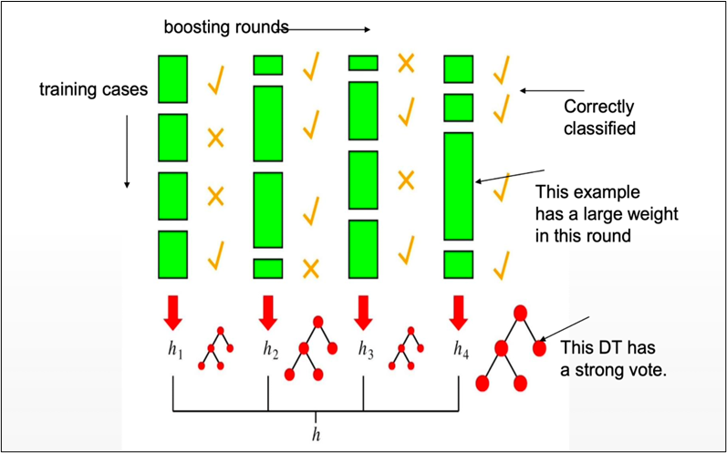
APPROACH OUTLINE:
- Start with a ML algorithm for finding the rough rules of thumb (a.k.a. “weak” or “base” algorithm)
- Call the base algorithm repeatedly, each time feeding it a different subset of the training examples
- The basic learning algorithm creates a new weak prediction rule each time it is invoked.
- After several rounds, the boosting algorithm must merge these weak rules into a single prediction rule that, hopefully, is considerably more accurate than any of the weak rules alone.
TWO KEY DETAILS :
- In each round, how is the distribution selected ?
- What is the best way to merge the weak rules into a single rule?
BOOSTING is classified into two types:
1] ADA BOOST
2] XG BOOST
As far as the Random forest is concerned it is said that it follows the bagging method, not a boosting method. As the name implies, boosting involves learning from others, which in turn increases learning. Random forests have trees that run in parallel. While creating the trees, there is no interaction between them.
Boosting helps us reduce the error by decreasing the bias whereas, on other hand, Bagging is a manner to decrease the variance within the prediction with the aid of generating additional information for schooling from the dataset using mixtures with repetitions to provide multi-sets of the original information.
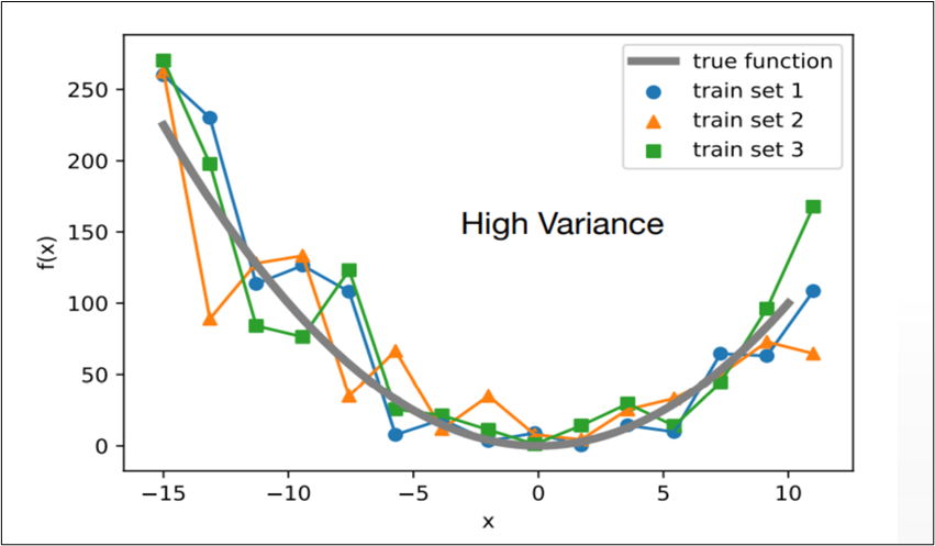
How Bagging helps with variance – A Simple Example
BAGGED TREES
- Decision Trees have high variance
- The resultant tree (model) is determined by the training data.
- (Unpruned) Decision Trees tend to overfit
- One option: Cost Complexity Pruning
BAG TREES
- Sample with replacement (1 Training set → Multiple training sets)
- Train model on each bootstrapped training set
- Multiple trees; each different : A garden ☺
- Each DT predicts; Mean / Majority vote prediction
- Choose # of trees to build (B)
ADVANTAGES
Reduce model variance / instability.
RANDOM FOREST : VARIABLE IMPORTANCE
VARIABLE IMPORTANCE :
▪ Each time a tree is split due to a variable m, Gini impurity index of the parent node is higher than that of the child nodes
▪ Adding up all Gini index decreases due to variable m over all trees in the forest, gives a measure of variable importance
IMPORTANT FEATURES AND HYPERPARAMETERS:
- Diversity :
- Immunity to the curse of dimensionality :
- Parallelization :
- Train-Test split :
- Stability :
- Gini significance (or mean reduction impurity) :
- Mean Decrease Accuracy :
FEATURES THAT IMPROVE THE MODEL’S PREDICTIONS and SPEED :
- maximum_features :
Increasing max features often increases model performance since each node now has a greater number of alternatives to examine.
- n_estimators :
The number of trees you wish to create before calculating the maximum voting or prediction averages. A greater number of trees improves speed but slows down your code.
- min_sample_leaf :
If you’ve ever designed a decision tree, you’ll understand the significance of the minimal sample leaf size. A leaf is the decision tree’s last node. A smaller leaf increases the likelihood of the model collecting noise in train data.
- n_jobs :
This option instructs the engine on how many processors it is permitted to utilise.
- random_state :
This argument makes it simple to duplicate a solution. If given the same parameters and training data, a definite value of random state will always provide the same results.
- oob_score:
A random forest cross validation approach is used here. It is similar to the leave one out validation procedure, except it is significantly faster.
LET’S SEE THE STEPS INVOLVED IN IMPLEMENTATION OF RANDOM FOREST ALGORITHM:
Step1: Choose T- number of trees to grow
Step2: Choose m<p (p is the number of total features) —number of features used to calculate the best split at each node (typically 30% for regression, sqrt(p) for classification)
Step3: For each tree, choose a training set by choosing N times (N is the number of training examples) with replacement from the training set
Step4: For each node, calculate the best split, Fully grown and not pruned.
Step5: Use majority voting among all the trees
Following is a full case study and implementation of all the principles we just covered, in the form of a jupyter notebook including every concept and all you ever wanted to know about RANDOM FOREST.
GITHUB Repository for this blog article: https://gist.github.com/Vidhi1290/c9a6046f079fd5abafb7583d3689a410