This is not a college course or something on deep learning with strict deadlines for assignments, so let’s take a detour from practical stuff and take a brief look at the history of neural networks.
The history of neural networks is also a big topic, which could be so long that I had to prepare another article series. And usually I am supposed to begin such articles with something like “The term ‘AI’ was first used by John McCarthy in Dartmouth conference 1956…” but you can find many of such texts written by people with much more experiences in this field. Therefore I am going to write this article from my point of view, as an intern writing articles on RNN, as a movie buff, and as one of many Japanese men who spent a great deal of childhood with video games.
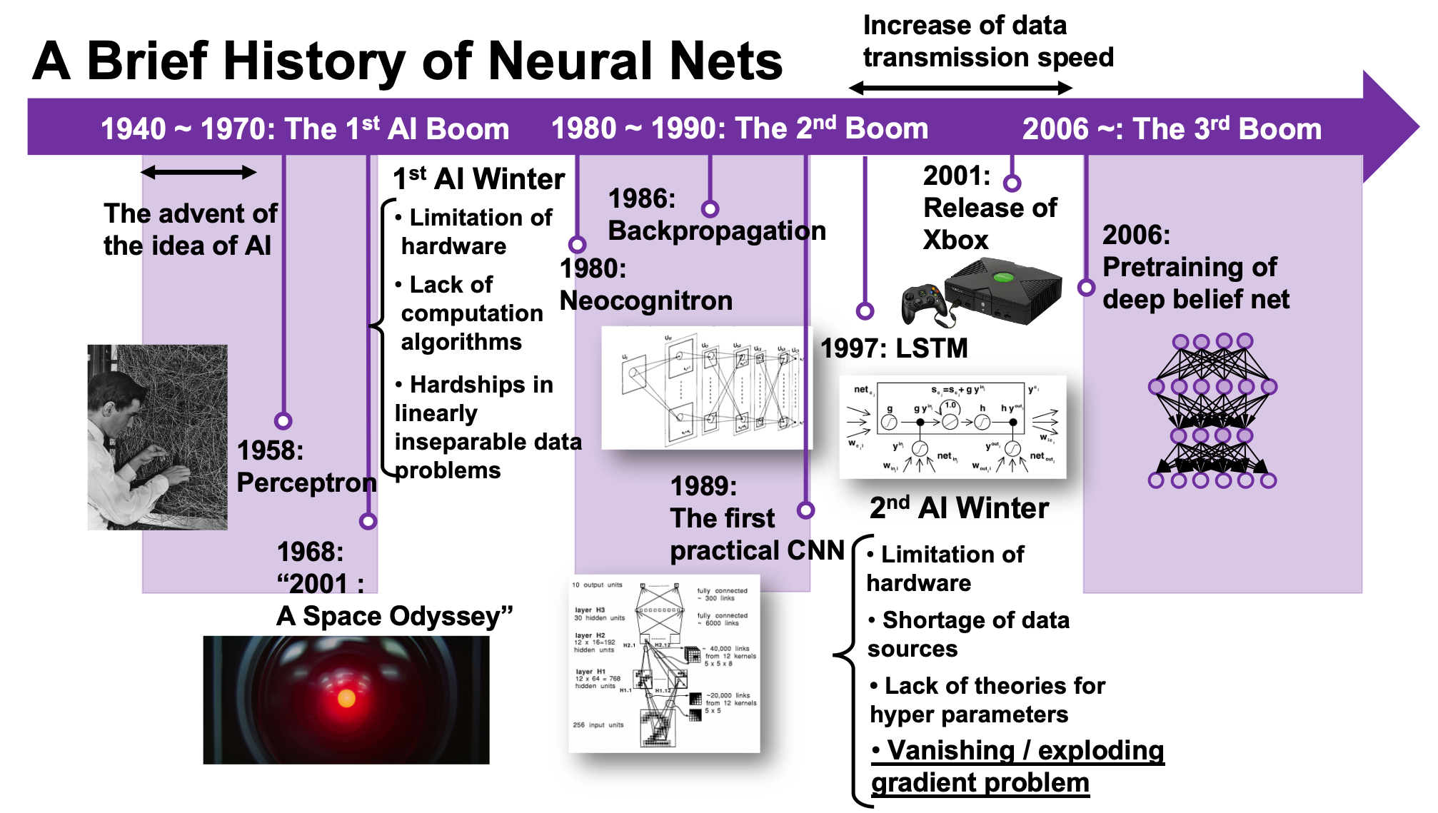
We are now in the third AI boom, and some researchers say this boom began in 2006. A professor in my university said there we are now in a kind of bubble economy in machine learning/data science industry, but people used to say “Stop daydreaming” to AI researchers. The second AI winter is partly due to vanishing/exploding gradient problem of deep learning. And LSTM was invented as one way to tackle such problems, in 1997.
1, First AI boom
In the first AI boom, I think people were literally “daydreaming.” Even though the applications of machine learning algorithms were limited to simple tasks like playing chess, checker, or searching route of 2d mazes, and sometimes this time is called GOFAI (Good Old Fashioned AI).
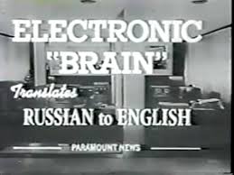
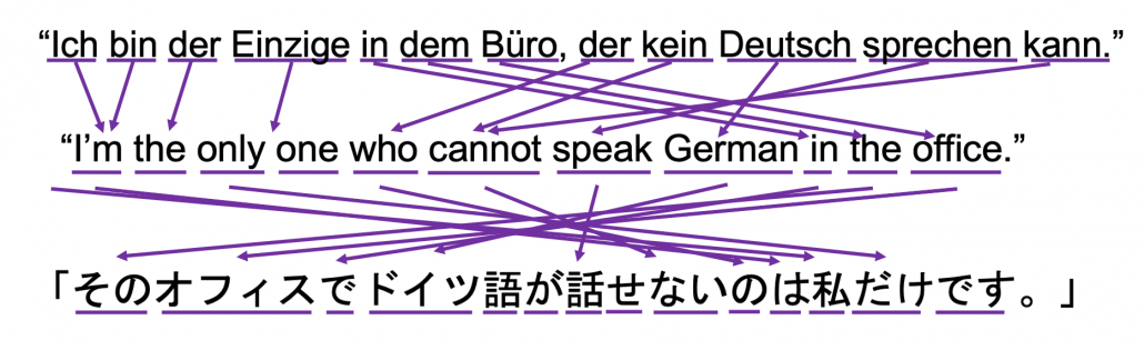
Even today when someone use the term “AI” merely for tasks with neural networks, that amuses me because for me deep learning is just statistically and automatically training neural networks, which are capable of universal approximation, into some classifiers/regressors. Actually the algorithms behind that is quite impressive, but the structure of human brains is much more complicated. The hype of “AI” already started in this first AI boom. Let me take an example of machine translation in this video. In fact the research of machine translation already started in the early 1950s, and of specific interest in the time was translation between English and Russian due to Cold War. In the first article of this series, I said one of the most famous applications of RNN is machine translation, such as Google Translation, DeepL. They are a type of machine translation called neural machine translation because they use neural networks, especially RNNs. Neural machine translation was an astonishing breakthrough around 2014 in machine translation field. The former major type of machine translation was statistical machine translation, based on statistical language models. And the machine translator in the first AI boom was rule base machine translators, which are more primitive than statistical ones.
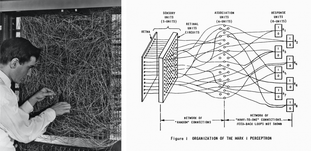
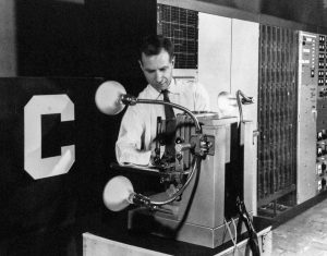 The most remarkable invention in this time was of course perceptron by Frank Rosenblatt. Some people say that this is the first neural network. Even though you can implement perceptron with a-few-line codes in Python, obviously they did not have Jupyter Notebook in those days. The perceptron was implemented as a huge instrument named Mark 1 Perceptron, and it was composed of randomly connected wires. I do not precisely know how it works, but it was a huge effort to implement even the most primitive type of neural networks. They needed to use a big lighting fixture to get a 20*20 pixel image using 20*20 array of cadmium sulphide photocells. The research by Rosenblatt, however, was criticized by Marvin Minsky in his book because perceptrons could only be used for linearly separable data. To make matters worse the criticism prevailed as that more general, multi-layer perceptrons were also not useful for linearly inseparable data (as I mentioned in the first article, multi-layer perceptrons, namely normal neural networks, can be universal approximators, which have potentials to classify/regress various types of complex data). In case you do not know what “linearly separable” means, imagine that there are data plotted on a piece of paper. If an elementary school kid can draw a border line between two clusters of the data with a ruler and a pencil on the paper, the 2d data is “linearly separable”….
With big disappointments to the research on “electronic brains,” the budget of AI research was reduced and AI research entered its first winter.
I think the frame problem(1969), by John McCarthy and Patrick J. Hayes, is also an iconic theory in the end of the first AI boom. This theory is known as a story of creating a robot trying to pull out its battery on a wheeled wagon in a room. The first prototype of the robot, named R1, naively tried to pull out the wagon form the room, and the bomb exploded. The problems was obvious: R1 was not programmed to consider the risks by taking each action, so the researchers made the next prototype named R1D1, which was programmed to consider the potential risks of taking each action. When R1D1 tried to pull out the wagon, it realized the risk of pulling the bomb together with the battery. But soon it started considering all the potential risks, such as the risk of the ceiling falling down, the distance between the wagon and all the walls, and so on, when the bomb exploded. The next problem was also obvious: R1D1 was not programmed to distinguish if the factors are relevant of irrelevant to the main purpose, and the next prototype R2D1 was programmed to do distinguish them. This time, R2D1 started thinking about “whether the factor is irrelevant to the main purpose,” on every factor measured, and again the bomb exploded. How can we get a perfect AI, R2D2?
The situation of mentioned above is a bit extreme, but it is said AI could also get stuck when it try to take some super simple actions like finding a number in a phone book and make a phone call. It is difficult for an artificial intelligence to decide what is relevant and what is irrelevant, but humans will not get stuck with such simple stuff, and sometimes the frame problem is counted as the most difficult and essential problem of developing AI. But personally I think the original frame problem was unreasonable in that McCarthy, in his attempts to model the real world, was inflexible in his handling of the various equations involved, treating them all with equal weight regardless of the particular circumstances of a situation. Some people say that McCarthy, who was an advocate for AI, also wanted to see the field come to an end, due to its failure to meet the high expectations it once aroused.
Not only the frame problem, but also many other AI-related technological/philosophical problems have been proposed, such as Chinese room (1980), the symbol grounding problem (1990), and they are thought to be as hardships in inventing artificial intelligence, but I omit those topics in this article.
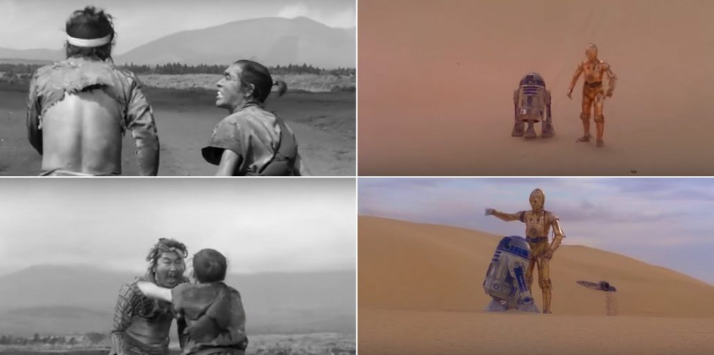
*The name R2D2 did not come from the famous story of frame problem. The story was Daniel Dennett first proposed the story of R2D2 in his paper published in 1984. Star Wars was first released in 1977. It is said that the name R2D2 came from “Reel 2, Dialogue 2,” which George Lucas said while film shooting. And the design of C3PO came from Maria in Metropolis(1927). It is said that the most famous AI duo in movie history was inspired by Tahei and Matashichi in The Hidden Fortress(1958), directed by Kurosawa Akira.
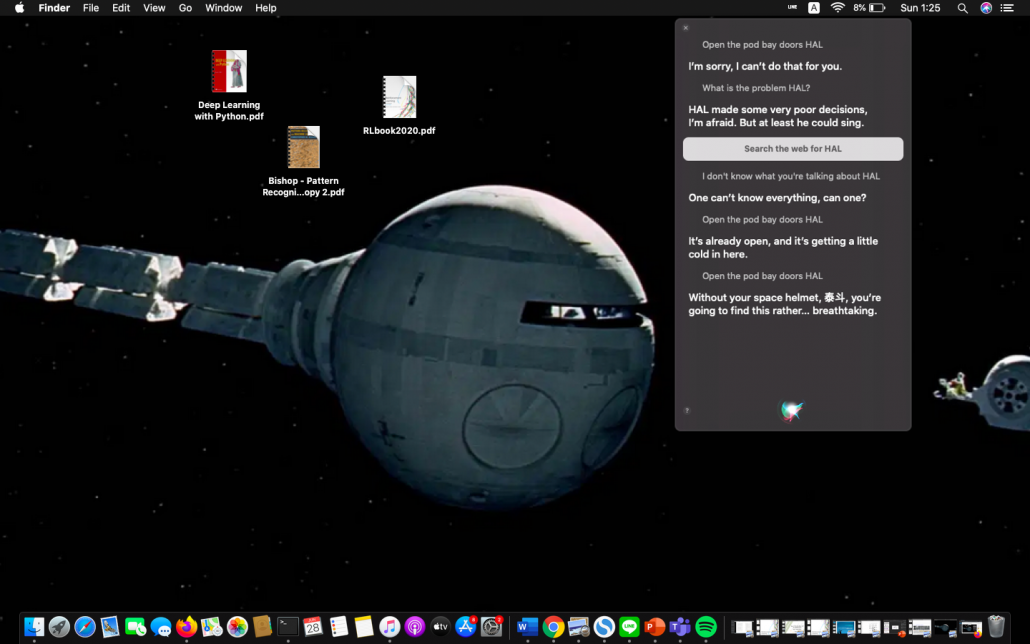
Interestingly, in the end of the first AI boom, 2001: A Space Odyssey, directed by Stanley Kubrick, was released in 1968. Unlike conventional fantasylike AI characters, for example Maria in Metropolis(1927), HAL 9000 was portrayed as a very realistic AI, and the movie already pointed out the risk of AI being insane when it gets some commands from several users. HAL 9000 still has been a very iconic character in AI field. For example when you say some quotes from 2001: A Space Odyssey to Siri you get some parody responses. I also thin you should keep it in mind that in order to make an AI like HAL 9000 come true, for now RNNs would be indispensable in many ways: you would need RNNs for better voice recognition, better conversational system, and for reading lips.
*Just as you cannot understand Monty Python references in Python official tutorials without watching Monty Python and the Holy Grail, you cannot understand many parodies in AI contexts without watching 2001: A Space Odyssey. Even thought the movie had some interview videos with some researchers and some narrations, Stanley Kubrick cut off all the footage and made the movie very difficult to understand. Most people did not or do not understand that it is a movie about aliens who gave homework of coming to Jupiter to human beings.
2, Second AI boom/winter
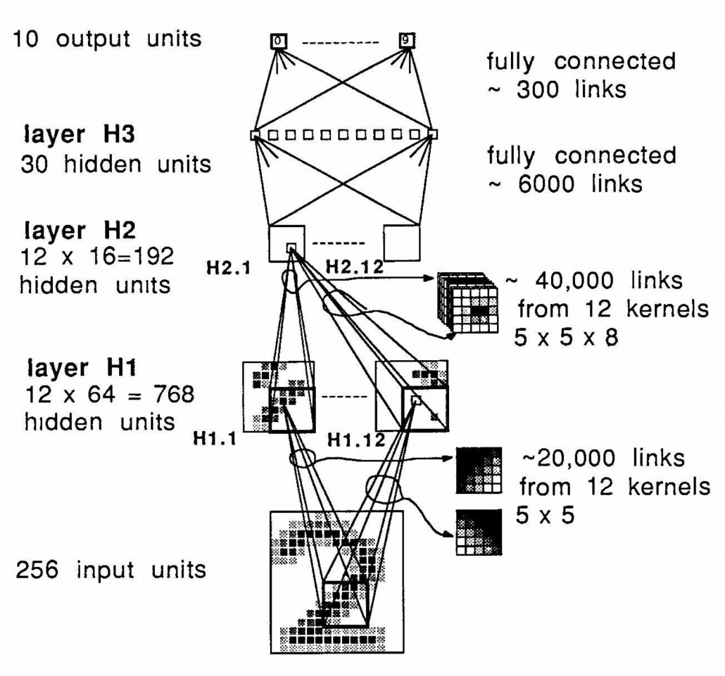
I am not going to write about the second AI boom in detail, but at least you should keep it in mind that convolutional neural network(CNN) is a keyword in this time. Neocognitron, an artificial model of how sight nerves perceive thing, was invented by Kunihiko Fukushima in 1980, and the model is said to be the origin on CNN. And Neocognitron got inspired by the Hubel and Wiesel’s research on sight nerves. In 1989, a group in AT & T Bell Laboratory led by Yann LeCun invented the first practical CNN to read handwritten digit.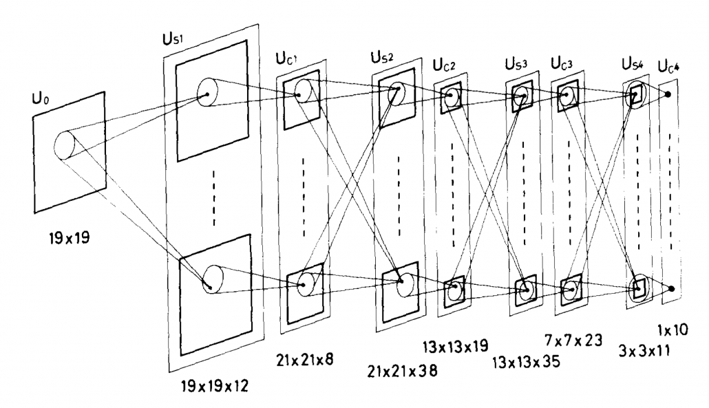
Another turning point in this second AI boom was that back propagation algorithm was discovered, and the CNN by LeCun was also trained with back propagation. LeCun made a deep neural networks with some layers in 1998 for more practical uses.
But his research did not gain so much attention like today, because AI research entered its second winter at the beginning of the 1990s, and that was partly due to vanishing/exploding gradient problem of deep learning. People knew that neural networks had potentials of universal approximation, but when they tried to train naively stacked neural nets the gradients, which you need to train neural networks, exponentially increased/decreased. Even though the CNN made by LeCun was the first successful case of “deep” neural nets which did not suffer from the vanishing/exploding gradient problem, deep learning research also stagnated in this time.
The ultimate goal of this article series is to understand LSTM at a more abstract/mathematical level because it is one of the practical RNNs, but the idea of LSTM (Long Short Term Memory) itself was already proposed in 1997 as an RNN algorithm to tackle vanishing gradient problem. (Exploding gradient problem is solved with a technique named gradient clipping, and this is easier than techniques for preventing vanishing gradient problems. I am also going to explain it in the next article.) After that some other techniques like introducing forget gate, peephole connections, were discovered, but basically it took some 20 years till LSTM got attentions like today. The reasons for that is lack of hardware and data sets, and that was also major reasons for the second AI winter.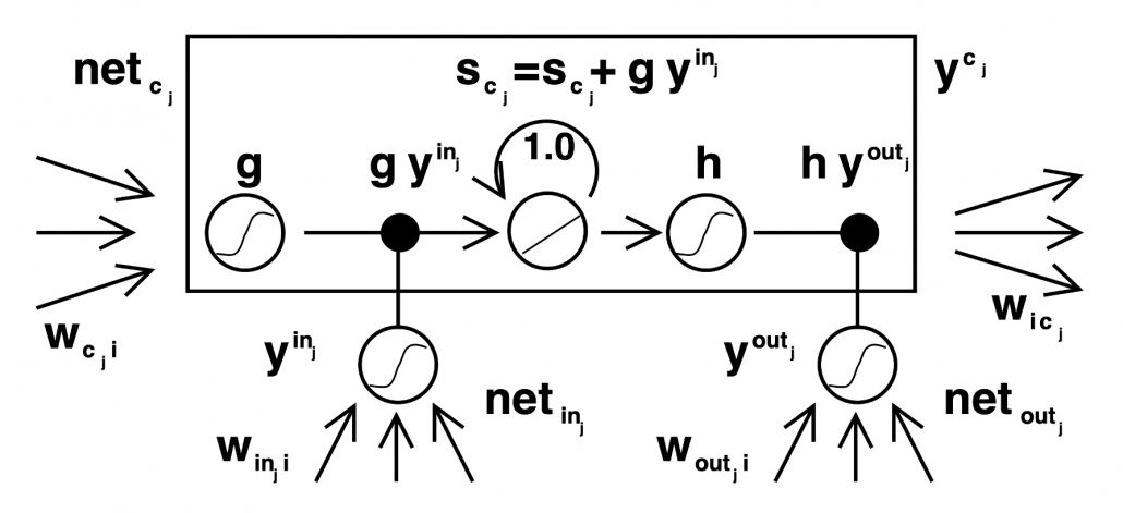
In the 1990s, the mid of second AI winter, the Internet started prevailing for commercial uses. I think one of the iconic events in this time was the source codes WWW(World Wide Web) were announced in 1993. Some of you might still remember that you little by little became able to transmit more data online in this time. That means people came to get more and more access to various datasets in those days, which is indispensable for machine learning tasks.
After all, we could not get HAL 9000 by the end of 2001, but instead we got Xbox console.
3, Video game industry and GPU
Even though research on neural networks stagnated in the 1990s the same period witnessed an advance in the computation of massive parallel linear transformations, due to their need in fields such as image processing.
Computer graphics move or rotate in 3d spaces, and that is also linear transformations. When you think about a car moving in a city, it is convenient to place the car, buildings, and other objects on a fixed 3d space. But when you need to make computer graphics of scenes of the city from a view point inside the car, you put a moving origin point in the car and see the city. The spatial information of the city is calculated as vectors from the moving origin point. Of course this is also linear transformations. Of course I am not talking about a dot or simple figures moving in the 3d spaces. Computer graphics are composed of numerous plane panels, and each of them have at least three vertexes, and they move on 3d spaces. Depending on viewpoints, you need project the 3d graphics in 3d spaces on 2d spaces to display the graphics on devices. You need to calculate which part of the panel is projected to which pixel on the display, and that is called rasterization. Plus, in order to get photophotorealistic image, you need to think about how lights from light sources reflect on the panel and projected on the display. And you also have to put some textures on groups of panels. You might also need to change color spaces, which is also linear transformations.
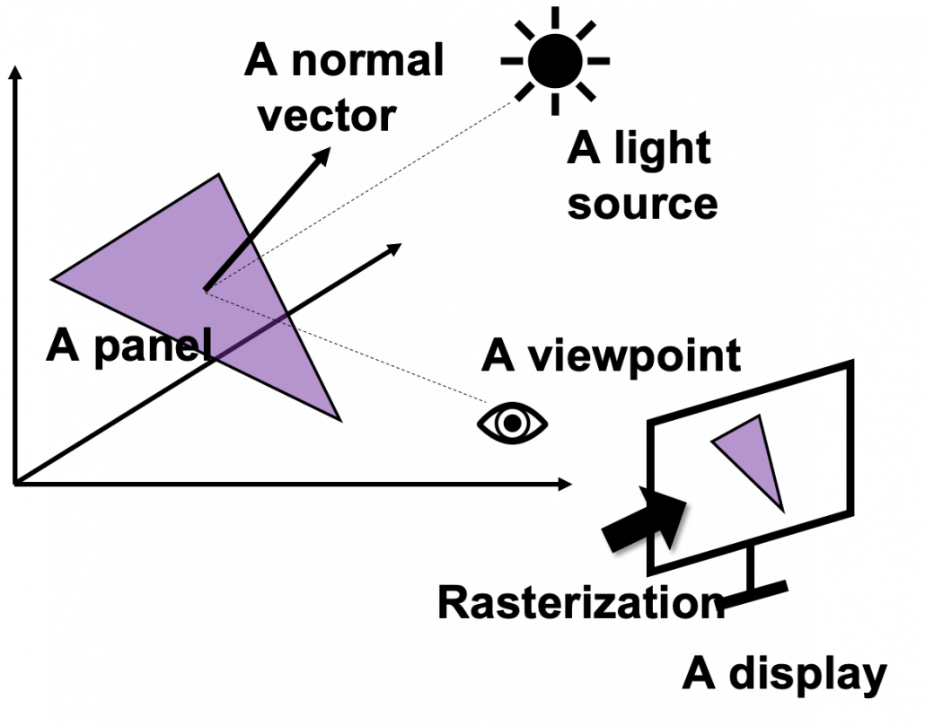
My point is, in short, you really need to do numerous linear transformations in parallel in image processing.
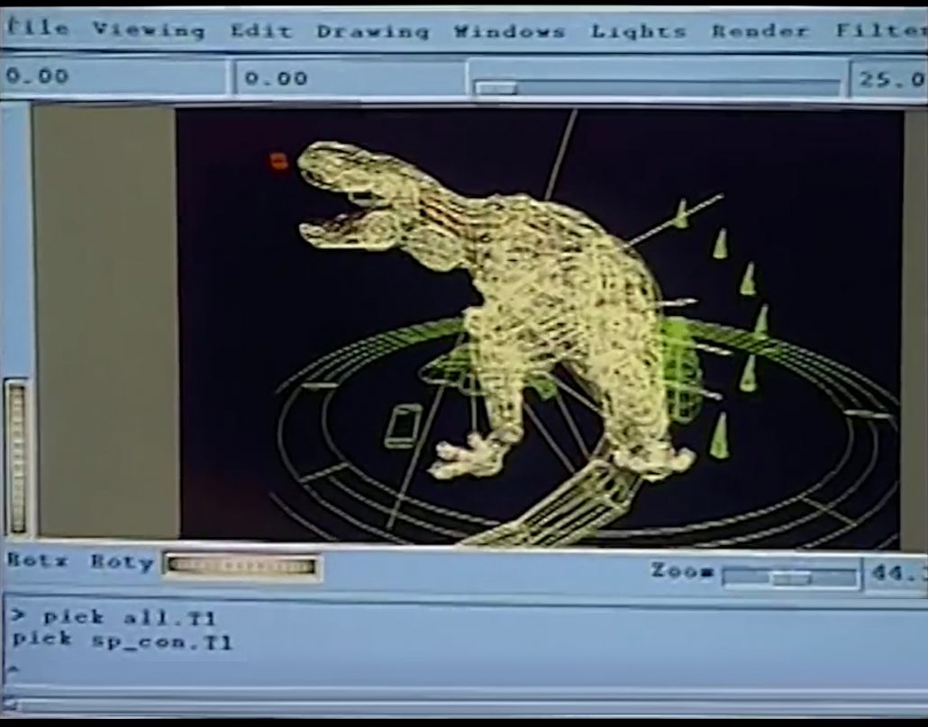
When it comes to the use of CGI in movies, two pioneer movies were released during this time: Jurassic Park in 1993, and Toy Story in 1995. It is famous that Pixar used to be one of the departments in ILM(Industrial Light and Magic), founded by George Lucas, and Steve Jobs bought the department. Even though the members in Pixar had not even made a long feature film in their lives, after trial and errors, they made the first CGI animated feature movie. On the other hand, in order to acquire funds for the production of Schindler’s List(1993), Steven Spielberg took on Jurassic Park(1993), consequently changing the history of CGI through this “side job.”
*I think you have realized that George Lucas is mentioned almost everywhere in this article. His influences on technologies are not only limited to image processing, but also sound measuring system, nonlinear editing system. Photoshop was also originally developed under his company. I need another article series for this topic, but maybe not in Data Science Blog.
Considering that the first wire-frame computer graphics made and displayed by computers appeared in the scene of displaying the wire frame structure of Death Star in a war room, in Star Wars: A New Hope, the development of CGI was already astonishing at this time. But I think deep learning owe its development more to video game industry.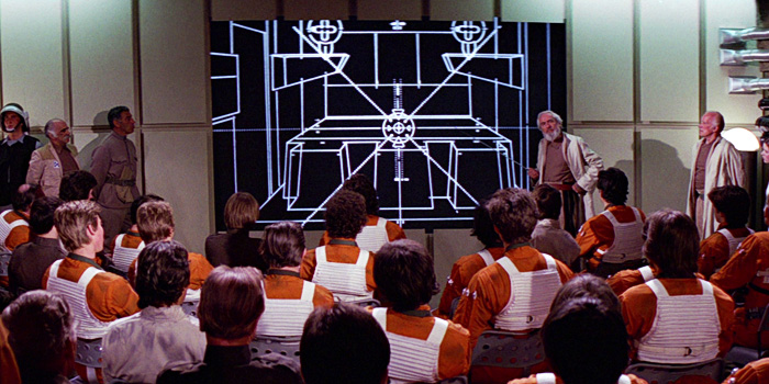
*I said that the Death Star scene is the first use of graphics made and DISPLAYED by computers, because I have to say one of the first graphics in movie MADE by computer dates back to the legendary title sequence of Vertigo(1958).
When it comes to 3D video games the processing unit has to constantly deal with real time commands from controllers. It is famous that GPU was originally specifically designed for plotting computer graphics. Video game market is the biggest in entertainment industry in general, and it is said that the quality of computer graphics have the strongest correlation with video games sales, therefore enhancing this quality is a priority for the video game console manufacturers.
One good example to see how much video games developed is comparing original Final Fantasy 7 and the remake one. The original one was released in 1997, the same year as when LSTM was invented. And recently the remake version of Final Fantasy 7 was finally released this year. The original one was also made with very big budget, and it was divided into three CD-ROMs. The original one was also very revolutionary given that the former ones of Final Fantasy franchise were all 2d video retro style video games. But still the computer graphics looks like polygons, and in almost all scenes the camera angle was fixed in the original one. On the other hand the remake one is very photorealistic and you can move the angle of the camera as you want while you play the video game.
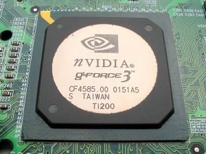
There were also fierce battles by graphic processor manufacturers in computer video game market in the 1990s, but personally I think the release of Xbox console was a turning point in the development of GPU. To be concrete, Microsoft adopted a type of NV20 GPU for Xbox consoles, and that left some room of programmability for developers. The chief architect of NV20, which was released under the brand of GeForce3, said making major changes in the company’s graphic chips was very risky. But that decision opened up possibilities of uses of GPU beyond computer graphics.
I think that the idea of a programmable GPU provided other scientific fields with more visible benefits after CUDA was launched. And GPU gained its position not only in deep learning, but also many other fields including making super computers.
*When it comes to deep learning, even GPUs have strong rivals. TPU(Tensor Processing Unit) made by Google, is specialized for deep learning tasks, and have astonishing processing speed. And FPGA(Field Programmable Gate Array), which was originally invented customizable electronic circuit, proved to be efficient for reducing electricity consumption of deep learning tasks.
*I am not so sure about this GPU part. Processing unit, including GPU is another big topic, that is beyond my capacity to be honest. I would appreciate it if you could share your view and some references to confirm your opinion, on the comment section or via email.
*If you are interested you should see this video of game fans’ reactions to the announcement of Final Fantasy 7. This is the industry which grew behind the development of deep learning, and many fields where you need parallel computations owe themselves to the nerds who spent a lot of money for video games, including me.
*But ironically the engineers who invented the GPU said they did not play video games simply because they were busy. If you try to study the technologies behind video games, you would not have much time playing them. That is the reality.
We have seen that the in this second AI winter, Internet and GPU laid foundation of the next AI boom. But still the last piece of the puzzle is missing: let’s look at the breakthrough which solved the vanishing /exploding gradient problem of deep learning in the next section.
4, Pretraining of deep belief networks: “The Dawn of Deep Learning”
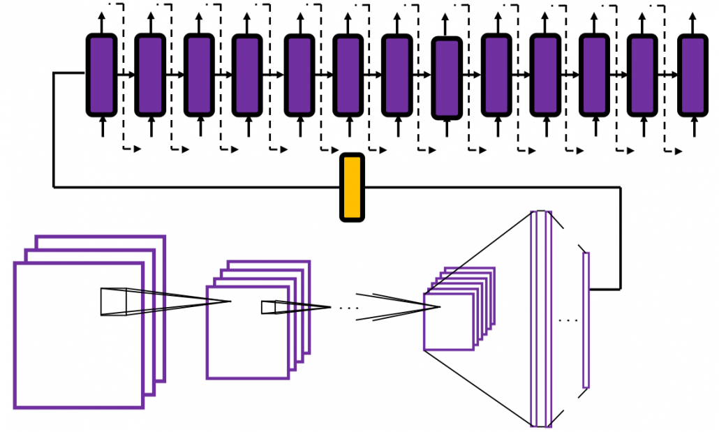
Some researchers say the invention of pretraining of deep belief network by Geoffrey Hinton was a breakthrough which put an end to the last AI winter. Deep belief networks are different type of networks from the neural networks we have discussed, but their architectures are similar to those of the neural networks. And it was also unknown how to train deep belief nets when they have several layers. Hinton discovered that training the networks layer by layer in advance can tackle vanishing gradient problems. And later it was discovered that you can do pretraining neural networks layer by layer with autoencoders.
*Deep belief network is beyond the scope of this article series. I have to talk about generative models, Boltzmann machine, and some other topics.
The pretraining techniques of neural networks is not mainstream anymore. But I think it is very meaningful to know that major deep learning techniques such as using ReLU activation functions, optimization with Adam, dropout, batch normalization, came up as more effective algorithms for deep learning after the advent of the pretraining techniques, and now we are in the third AI boom.
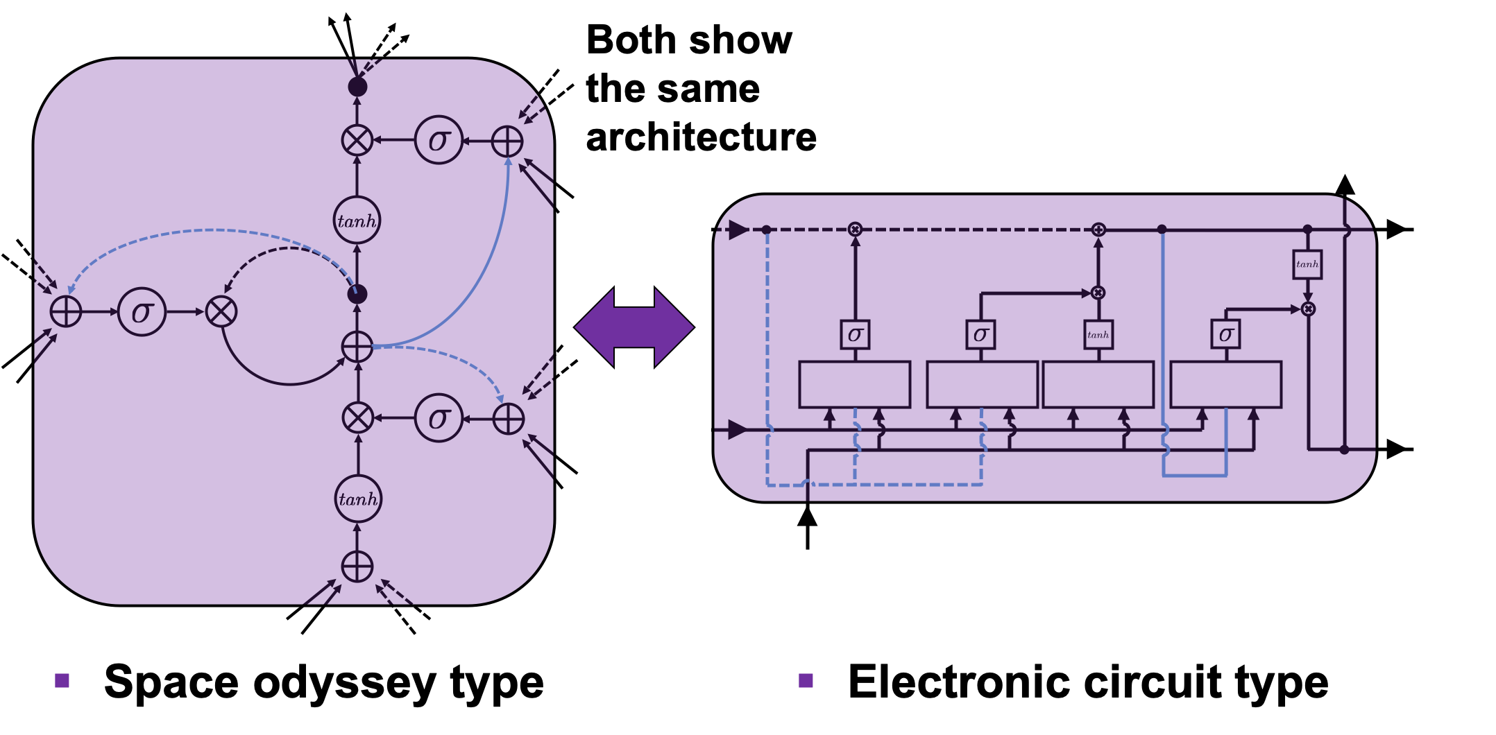
In the next next article we are finally going to work on LSTM. Specifically, I am going to offer a clearer guide to a well-made paper on LSTM, named “LSTM: A Search Space Odyssey.”
* I make study materials on machine learning, sponsored by DATANOMIQ. I do my best to make my content as straightforward but as precise as possible. I include all of my reference sources. If you notice any mistakes in my materials, including grammatical errors, please let me know (email: yasuto.tamura@datanomiq.de). And if you have any advice for making my materials more understandable to learners, I would appreciate hearing it.
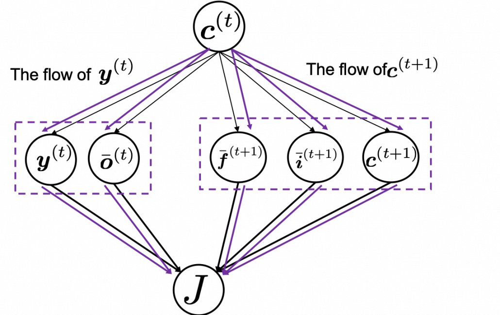
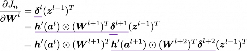
 , and relations of the functions are displayed as the graphical model at the left side of the figure below. Variables are a type of function, so you should think that every node in graphical models denotes a function. Arrows in purple in the right side of the chart show how information propagate in differentiation.
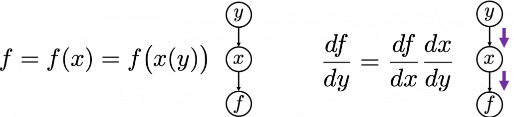
 , which has two variances
  and
and  . And both of the variances also share two variances
  and
and  . When you take partial differentiation of
  . The variance
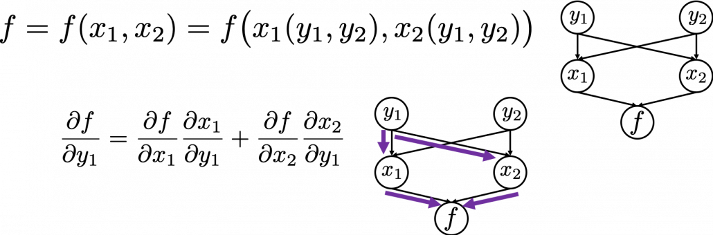
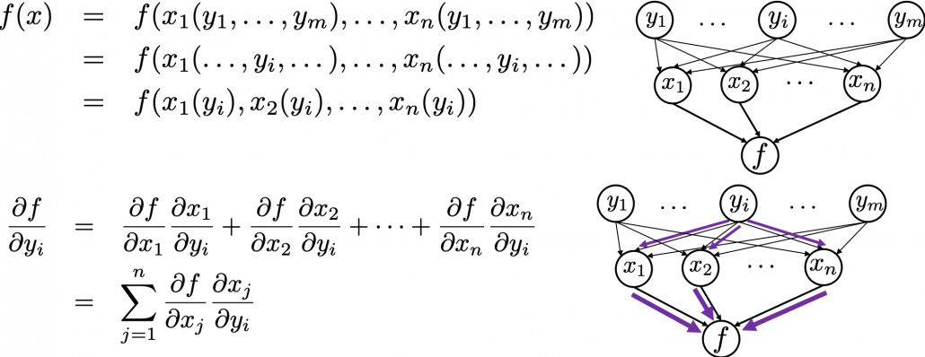
 , the partial differentiation has
  terms in total because
  , gradients of the error function with respect to parameters, at every time step. But you have to be careful that even though these gradients depend on time steps, the parameters
  do not depend on time steps.
 because parameters themselves do not depend on time.
  propagate backward to all the
  . Conversely, in order to calculate
  . In the chart you need arrows of errors in purple for the gradient in a purple frame, orange arrows for gradients in orange frame, red arrows for gradients in red frame. And you need to sum up
  , and you need this gradient
  to renew parameters, one time.

 means. Neurons depend on time steps, but parameters do not depend on time steps. So if
  are neurons,
  , but when
  should be rather denoted like
  . In the
  are not used as parameters, but in
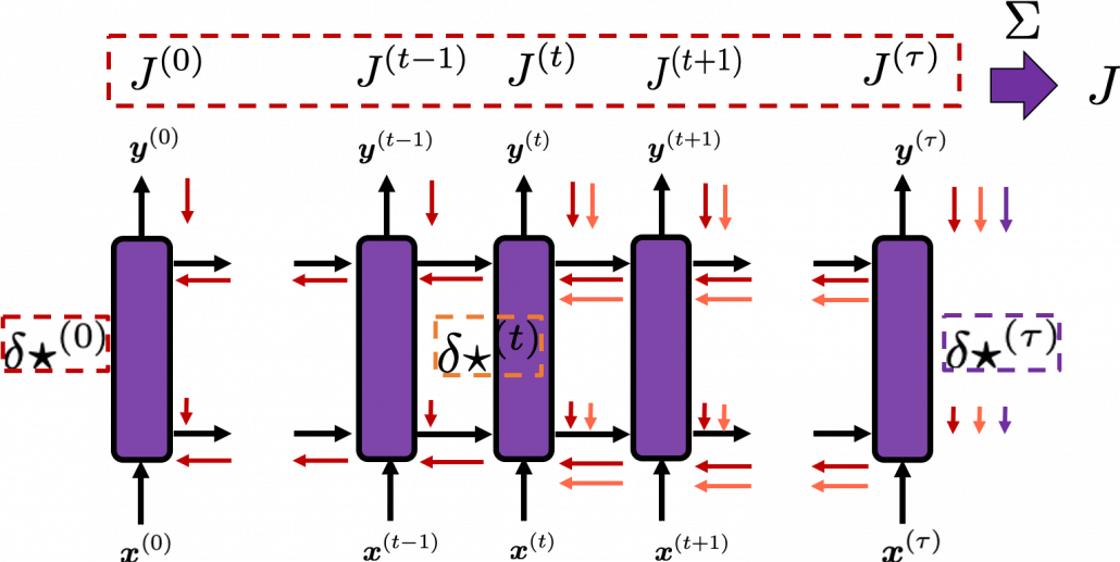
 as below. Unlike the last article, I also added the terms of peephole connections in the equations below, and I also added the variances
  for convenience.


 , where
  . And just as backprop of simple RNNs, in order to calculate gradients with respect to parameters, you need to calculate errors of neurons, that is gradients of error functions with respect to neurons, such as
  .
. , but the equation for this error is the most difficult, so I recommend you to put it aside for now. After calculating
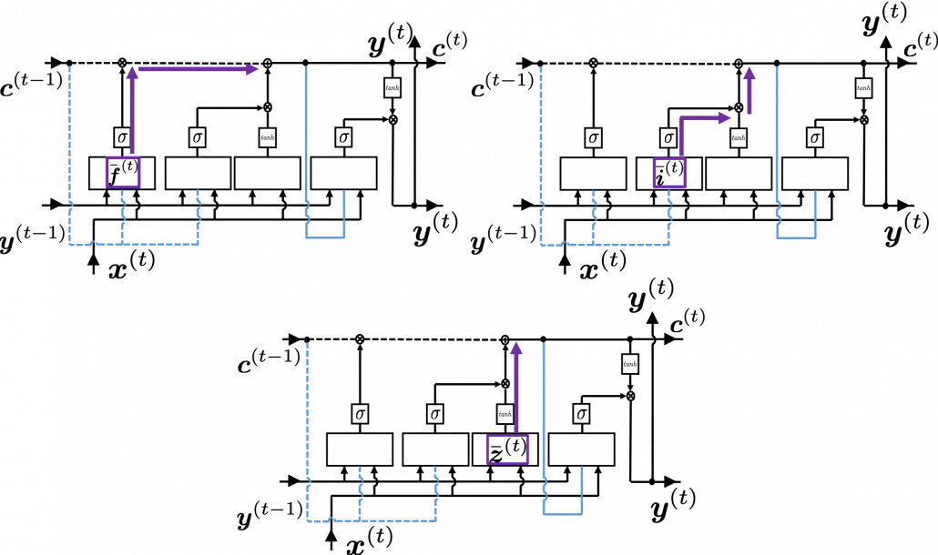
  . If you see the LSTM block below as a graphical model which I introduced, the information of
  flow like the purple arrows. That means,
  only via
  , and this structure is equal to the first graphical model which I have introduced above. And if you calculate
  .
. is an index of an element of vectors. If you can calculate element-wise gradients, it is easy to understand that as differentiation of vectors and matrices.
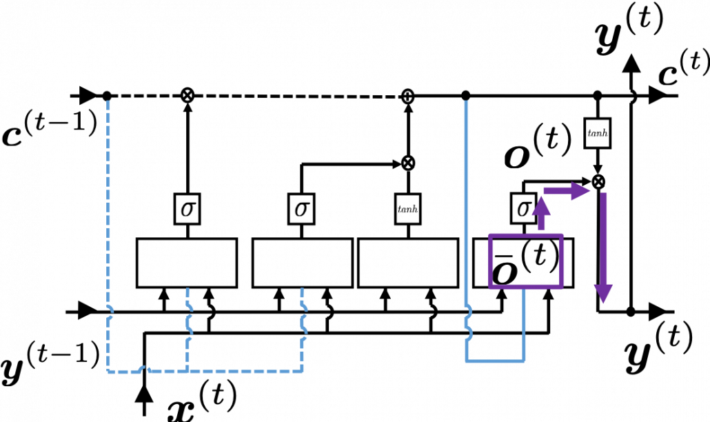
 , and chain rules are very important in this process. The flow of
  , and the one flows to
  . And the stream from
  to
to  ,
,  , and the one which directly converges as
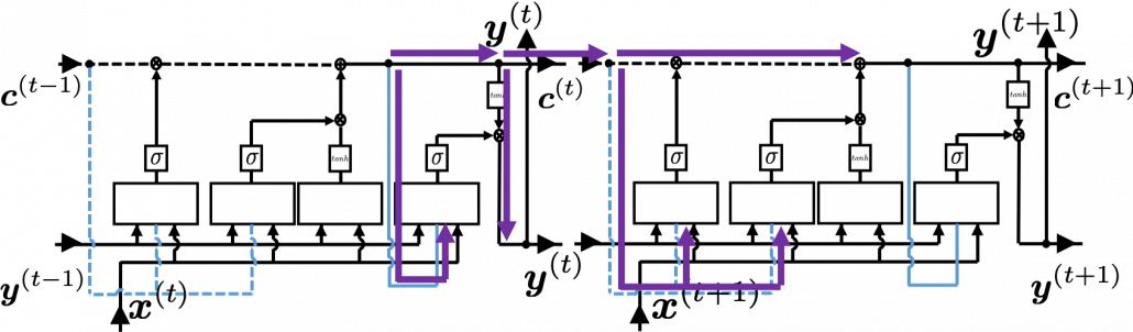
 element-wise as below.
 . In the case above, in the part
  the partial differential operator only affects
  of
of  , and in the part
  , the partial differential operator
  only affects the part
  of the term
  . In the
  part, only
  , in the
  part, only
  , and in the
  part, only
  of
of  ,
,  ,
,  are also relatively straigtforward as calculating
  . They all use the first type of chain rule in the first section. Thereby you can get these gradients:
  ,
,  , and
, and  .
.
 , and the flows of
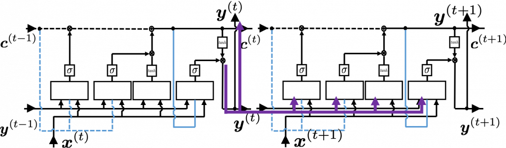


 . Let’s consider the gradient of
  , that is the error flowing from
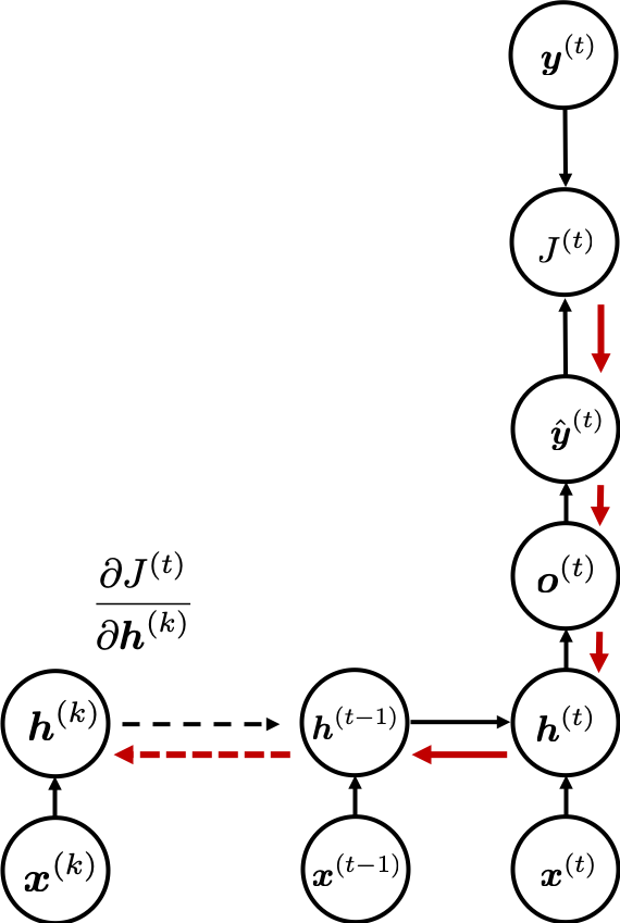
 , where
  .
. , but it seems that many study materials and web sites are mistaken in this point.
 . If you take norms of the members you get an equality
  . I will not go into detail anymore, but it is known that according to this inequality, multiplication of weight vectors exponentially converge to 0 or to infinite number.
 is the main factor causing vanishing/exploding gradient problems. In case of LSTM,
  is an equivalent. For simplicity, let’s calculate only
  , which is equivalent to
  of simple RNN backprop.
 affects in the chain rule above. That is, you need to calculate
  , and the partial differential operator only affects
  . I think this is not a correct mathematical notation, but please forgive me for doing this for convenience.
 is every effective. The unaffected value of can directly
 is a gradient at the time step
  is the maximum size of the “step.”
 , that means the loss function
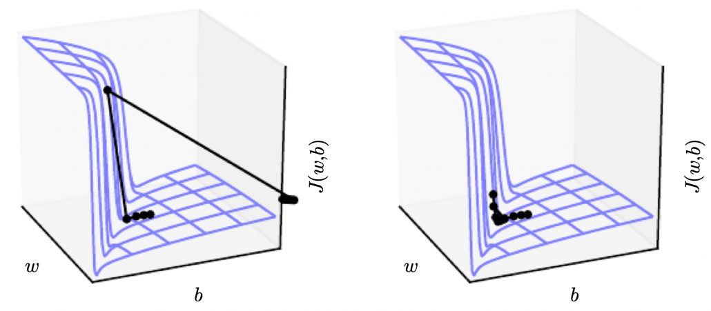
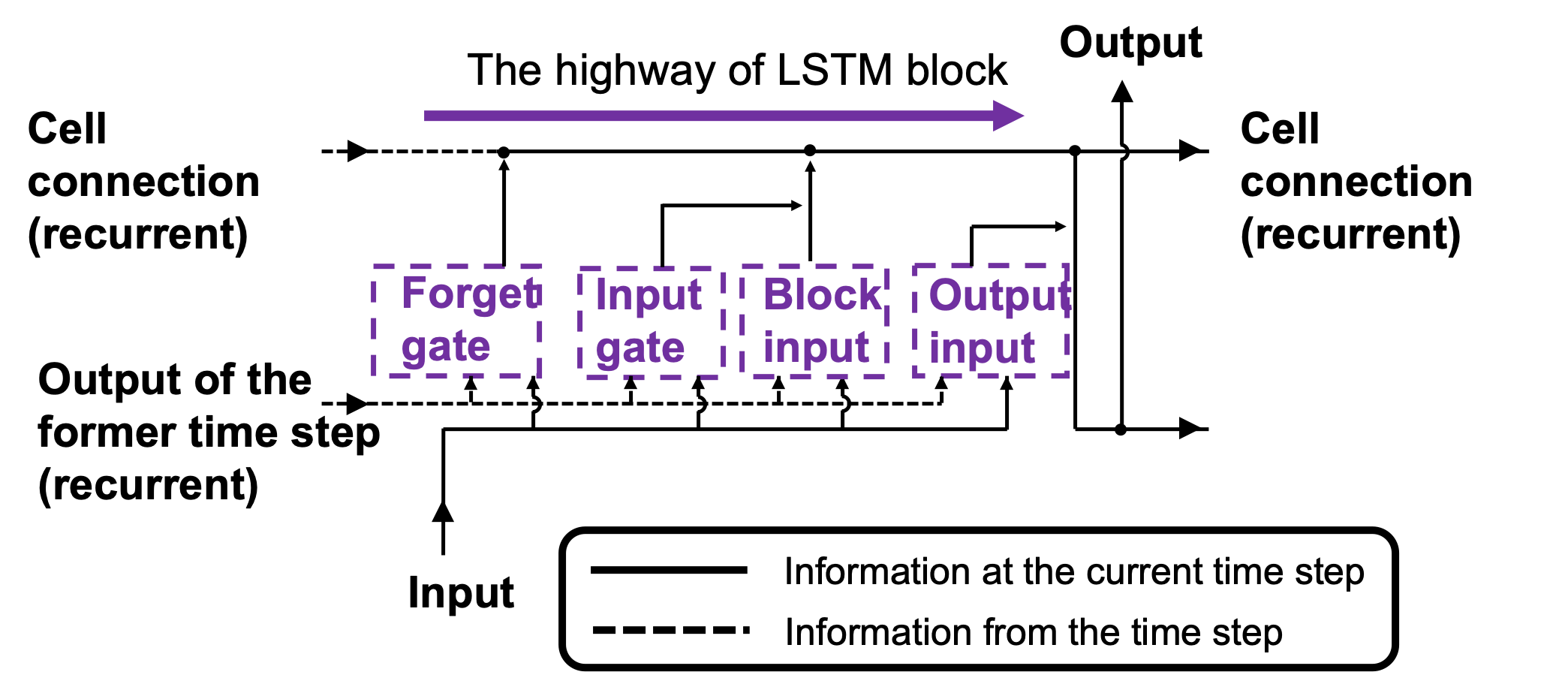
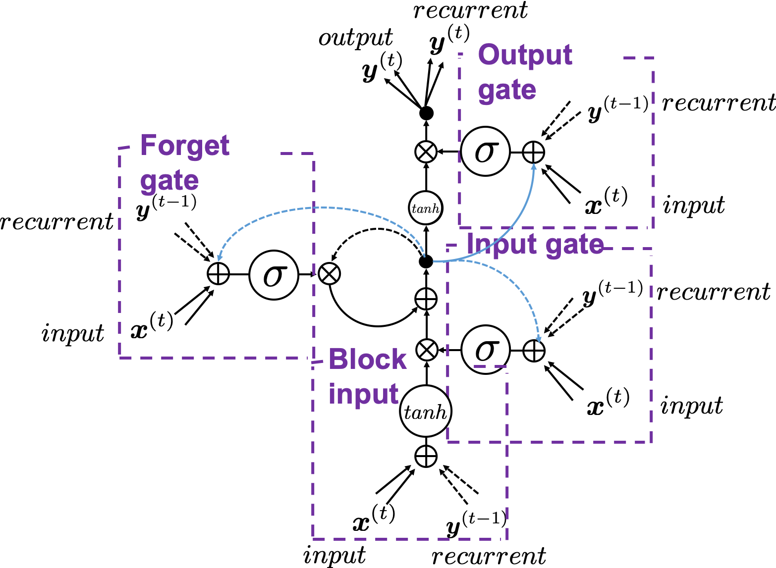
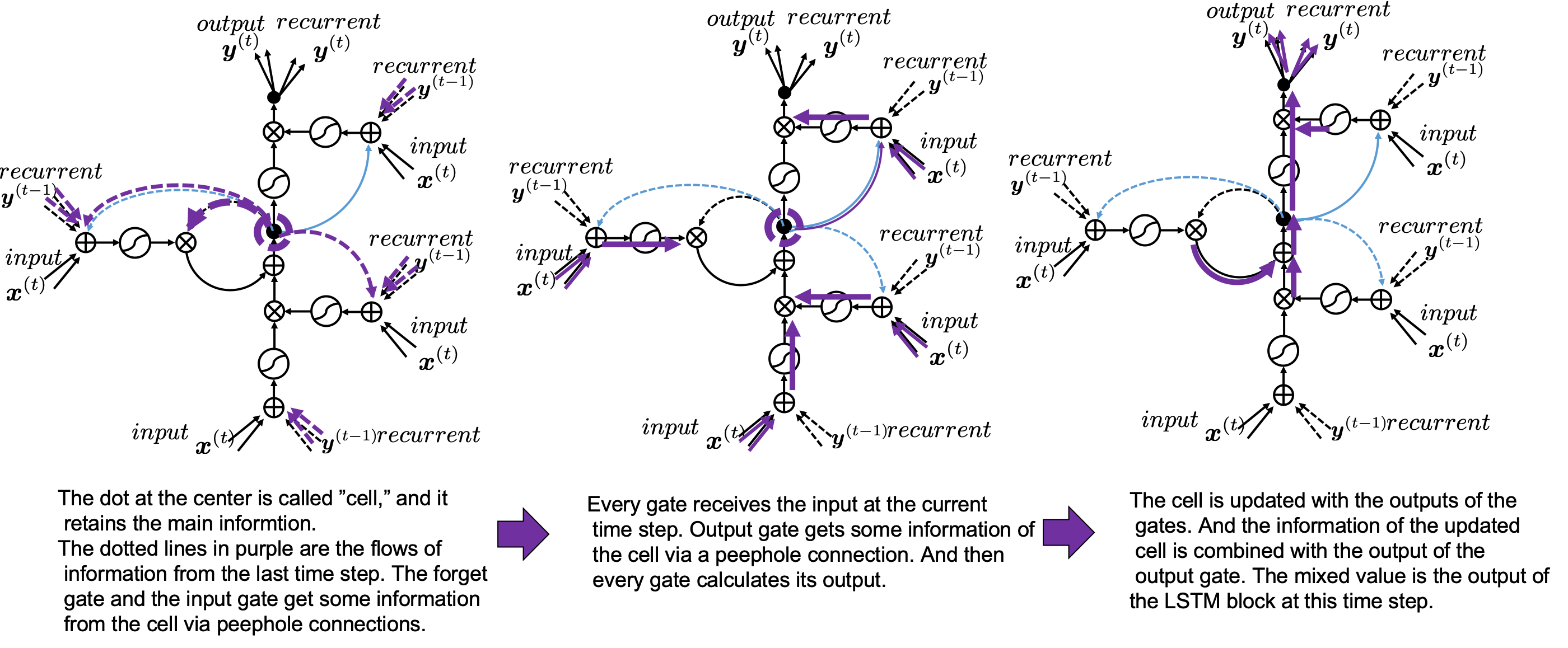
 , the output at the last time step, and
  , via recurrent connections. The block at time step
  , and it separately goes through each gate, together with
  to the next LSTM block via recurrent connections.
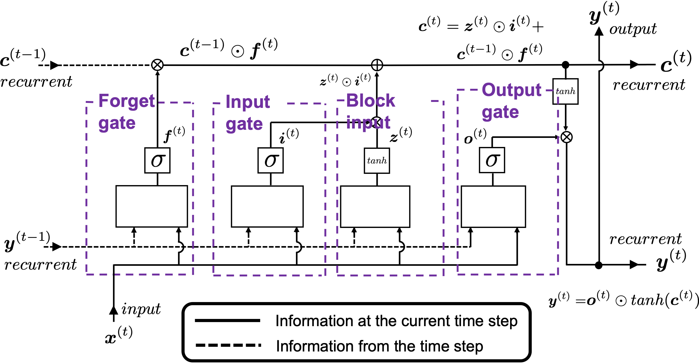


 . This is a very simple operator. This operator produces an elementwise product of two vectors or matrices with identical shape.
![[0, 1]](https://data-science-blog.com/en/wp-content/ql-cache/quicklatex.com-caffaae885a1287e3dfc31bfb1cd0694_l3.png "Rendered by QuickLaTeX.com") or
or ![[-1, 1]](https://data-science-blog.com/en/wp-content/ql-cache/quicklatex.com-96395345c57f8928c42918c656dd1364_l3.png "Rendered by QuickLaTeX.com") with activation functions. You can see that the input gate and the block input give new information to the cell. The part
with activation functions. You can see that the input gate and the block input give new information to the cell. The part  means that the output of the forget gate “forgets” the cell of the last time step by multiplying the values from 0 to 1 elementwise. And the cell
  and the output of the output gate “suppress” the activated value of
  , LSTMs forget nothing, retain information of inputs at every time step, and gives out everything. And if all the outputs of every gate are always
  , LSTMs forget everything, receive no inputs, and give out nothing.
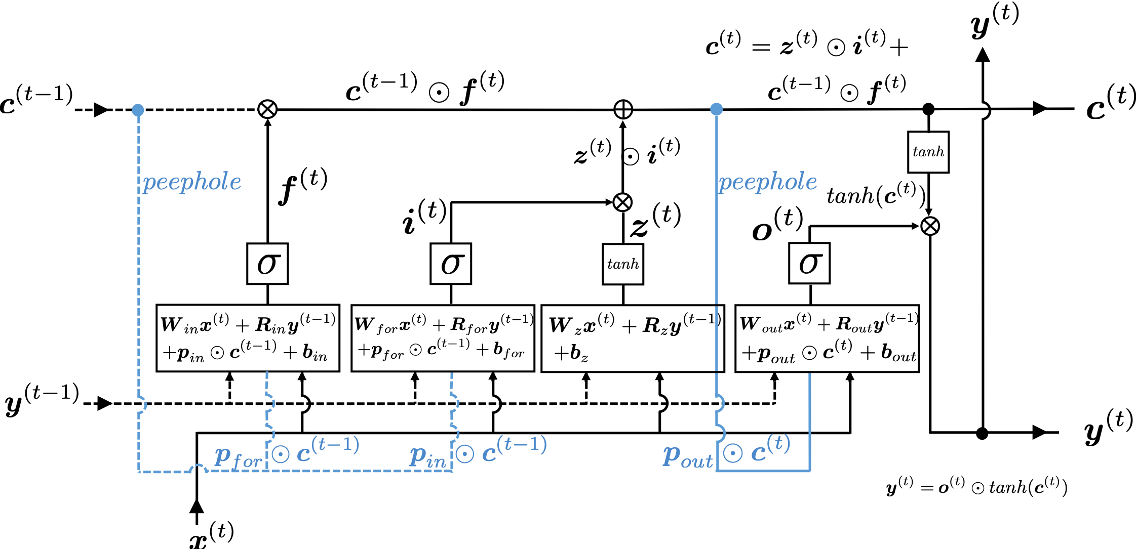

 , then
  is a variant, and
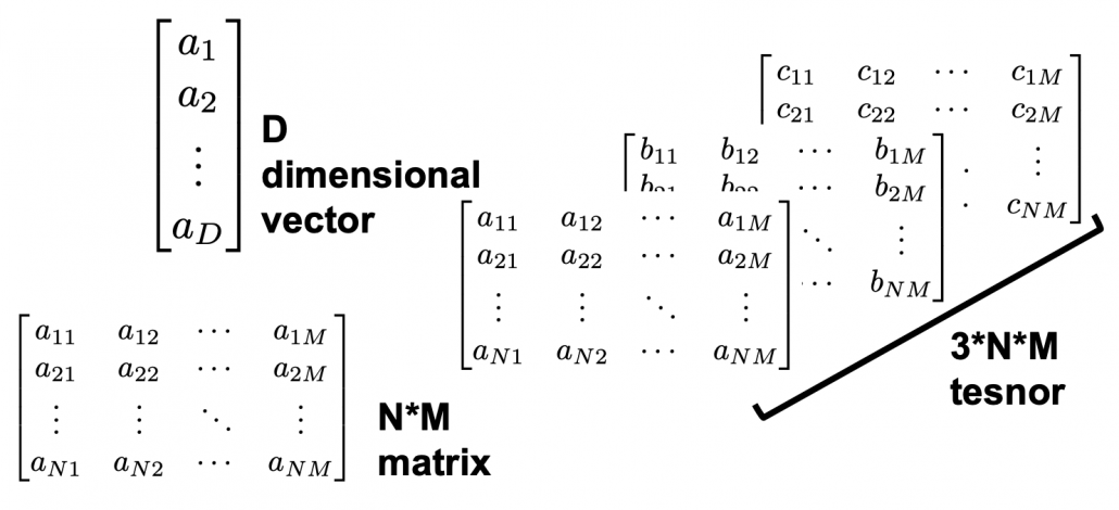
  are parameters. In case of classical machine learning algorithms, the number of those parameters are very limited because they were originally designed manually. Such functions for classical machine learning is useful for features found by humans, after trial and errors(feature engineering is a field of finding such effective features, manually). You adjust those parameters based on how different the outputs(estimated outcome of classification/regression) are from supervising vectors(the data prepared to show ideal answers).
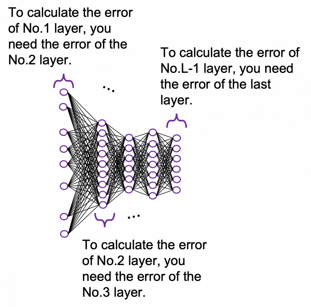
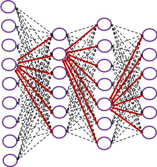
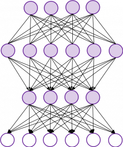
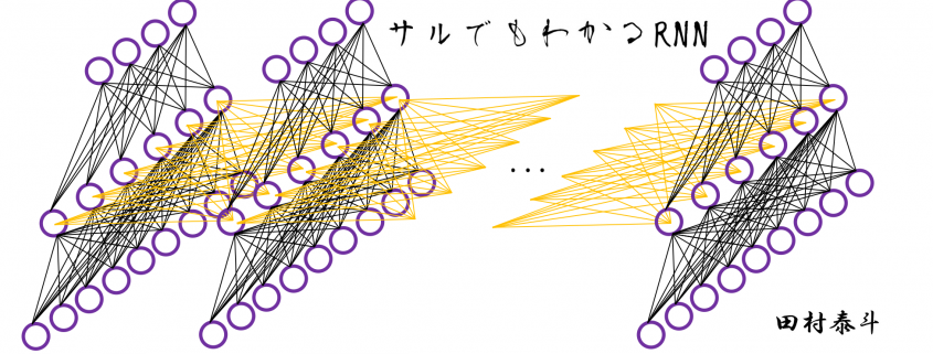
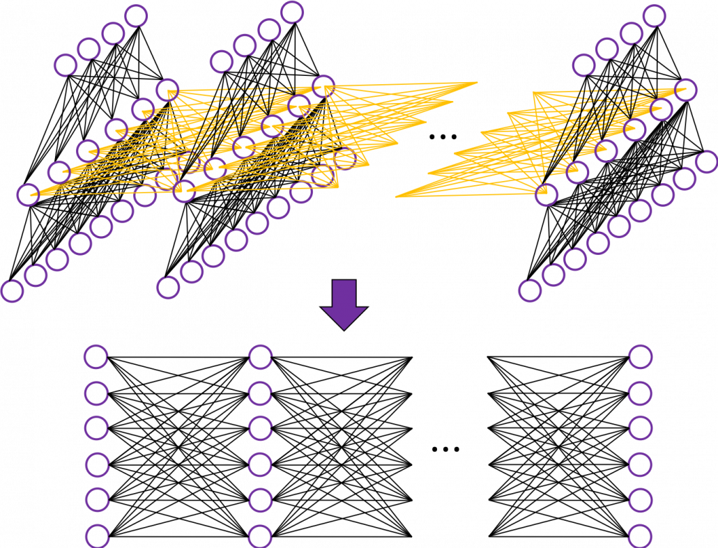
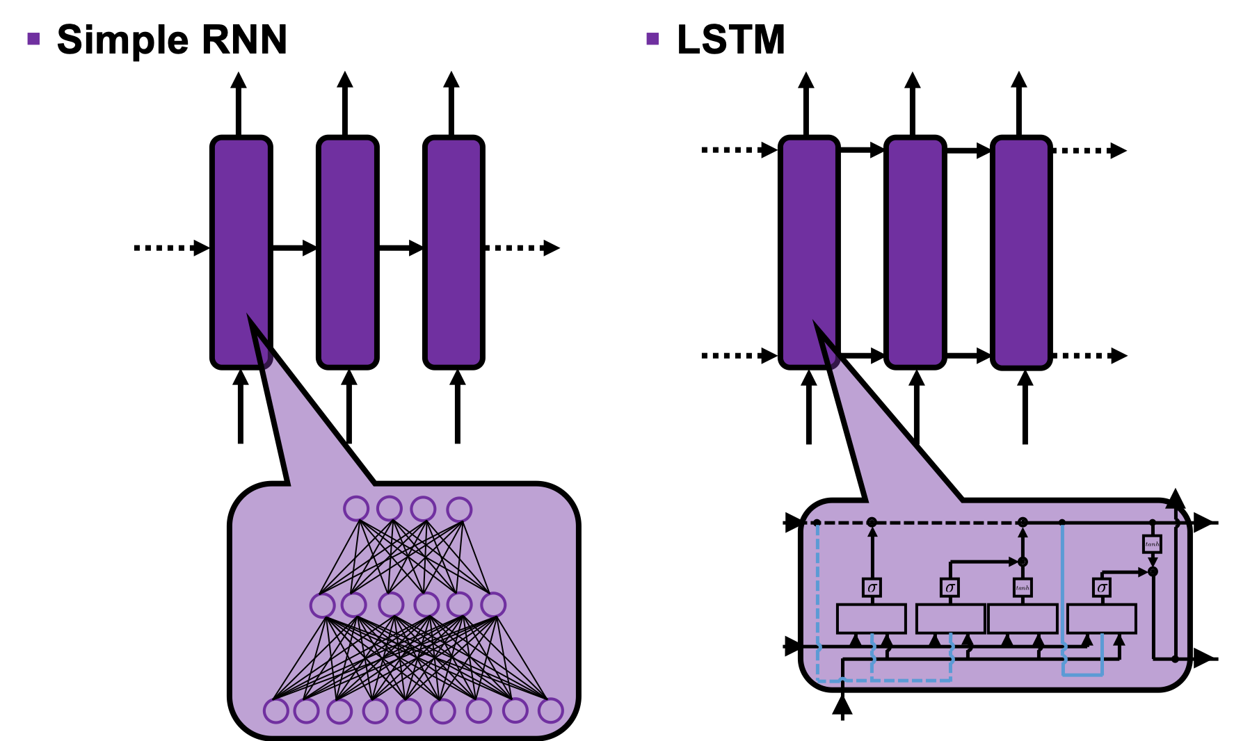
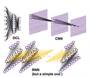
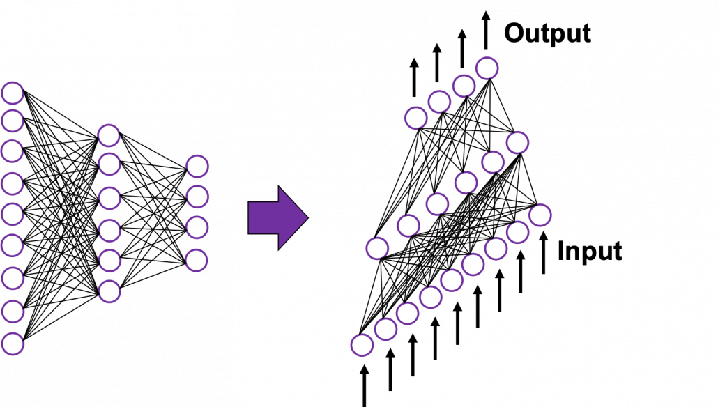 In fact the simple RNN which we are going to look at in this article has only three layers. From now on imagine that inputs of RNN come from the bottom and outputs go up. But RNNs have to keep information of earlier times steps during upcoming several time steps because as I mentioned in the last article RNNs are used for sequence data, the order of whose elements is important. In order to do that, information of the neurons in the middle layer of RNN propagate forward to the middle layer itself. Therefore in one time step of forward propagation of RNN, the input at the time step propagates forward as normal DCL, and the RNN gives out an output at the time step. And information of one neuron in the middle layer propagate forward to the other neurons like yellow arrows in the figure. And the information in the next neuron propagate forward to the other neurons, and this process is repeated. This is called recurrent connections of RNN.
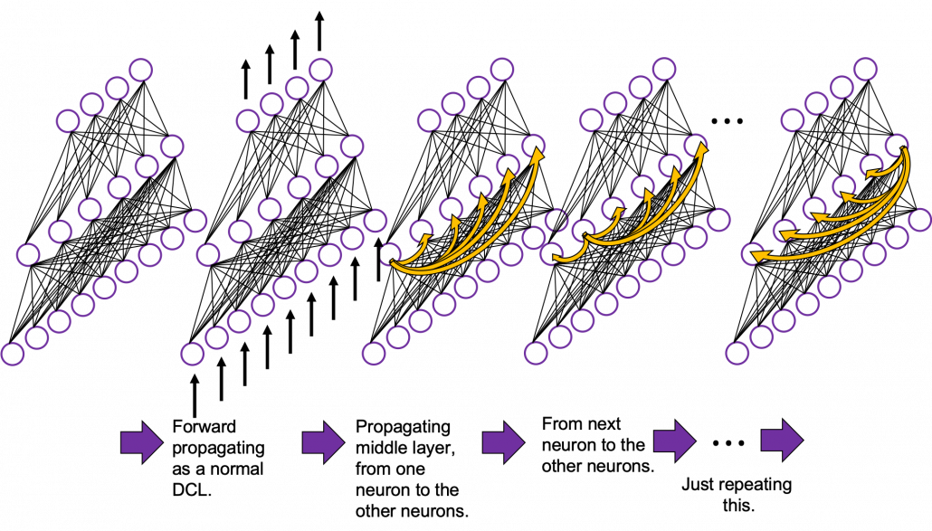
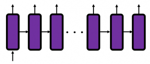
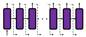
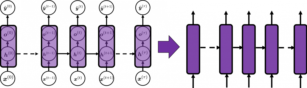
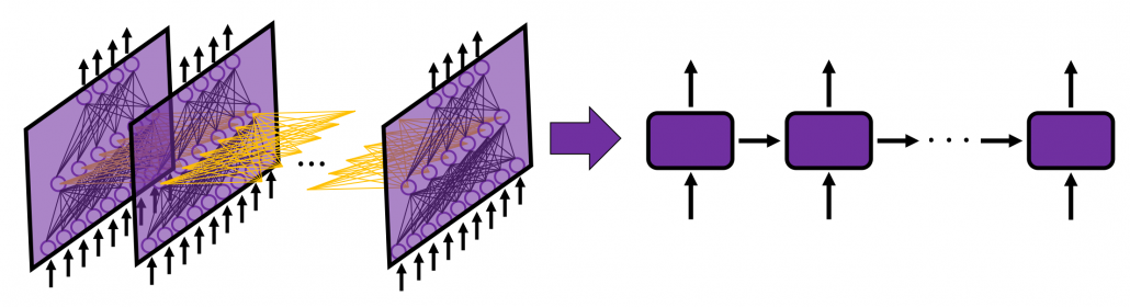
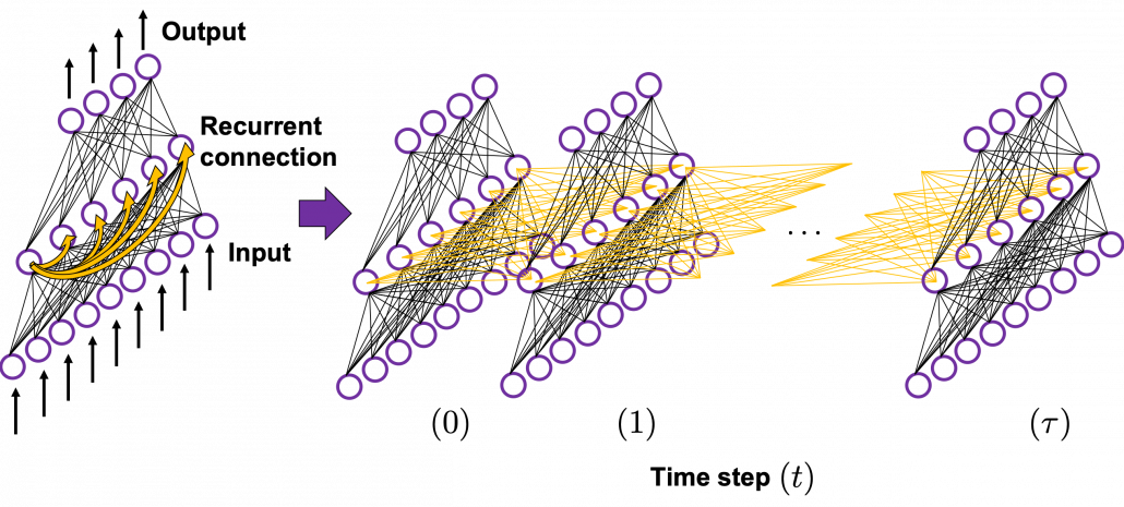 In many situations, RNNs are simplified as below. If you have read through this article until this point, I bet you gained some better understanding of RNNs, so you should little by little get used to this more abstract, blackboxed way of showing RNN.
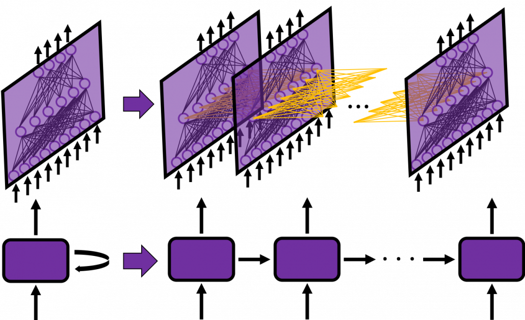
 .
.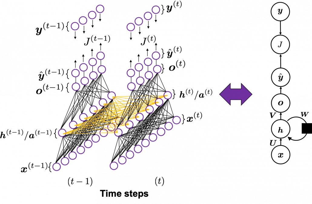
 at time step
 (The notation on the
  is called “hat,” and it means that the value is an estimated value. Whatever machine learning tasks you work on, the outputs of the functions are just estimations of ideal outcomes. You need to adjust parameters for better estimations. You should always be careful whether it is an actual value or an estimated value in the context of machine learning or statistics). But the most important parts are the middle layers.
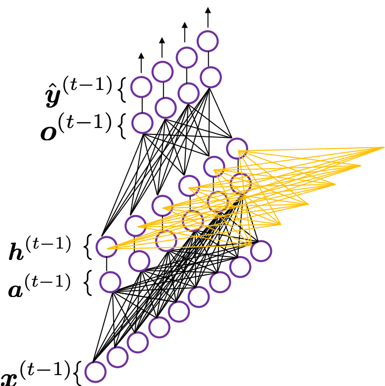
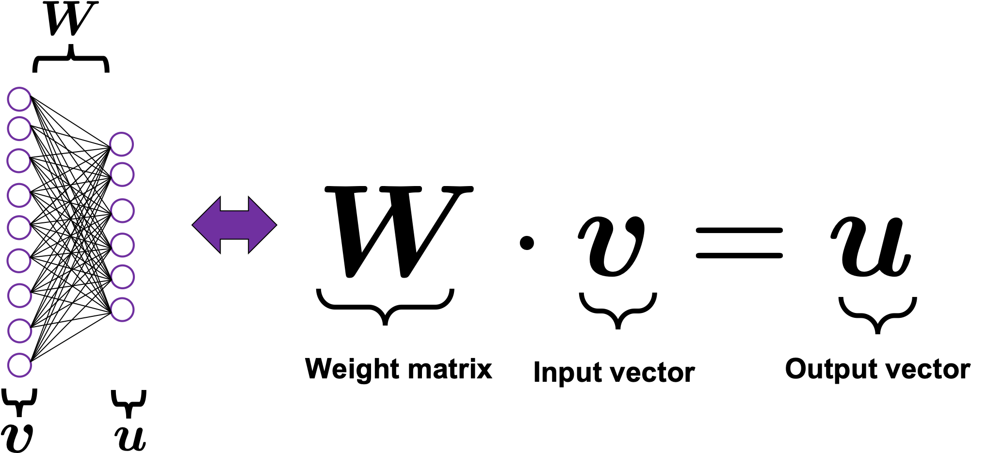
 is just linear summations of
  is a combination of activated values of
  from the last time step, with recurrent connections. The values of
  , and the other is recurrent connections to
  .
. , and weights
  , then
  is a linear summation of
  , and its weights are
  .
. and
and  , you should clearly make an image of connections between two layers of a neural network. You can also say each element of
  is a linear summations all the elements of
  , and
, and 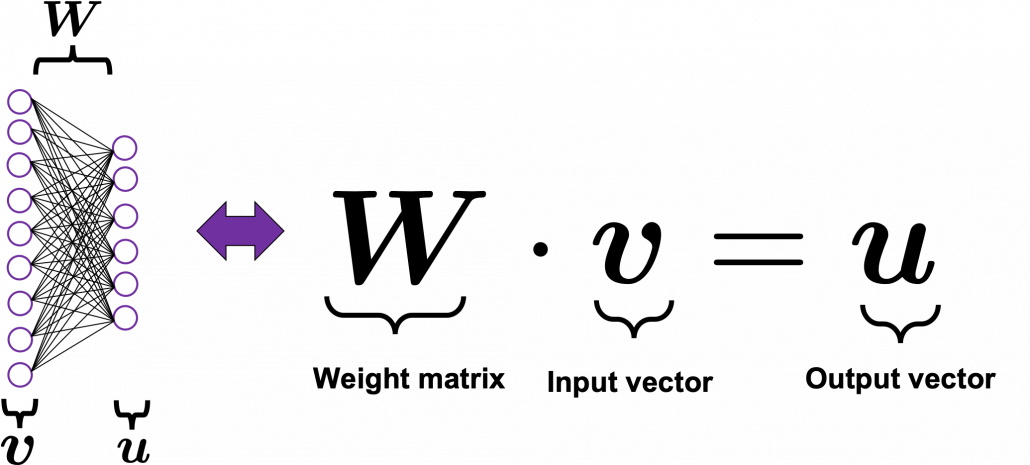
 , at every time step.
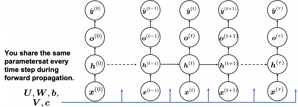
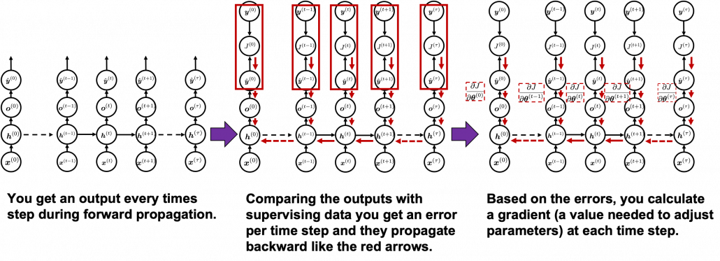 You need all the gradients to adjust parameters, but you do not necessarily need all the errors to calculate those gradients. Gradients in the context of machine learning mean partial derivatives of error functions (in this case
  is denoted as
  . And another confusing point in many textbooks, including the MIT one, is that they give an impression that parameters depend on time steps. For example some study materials use notations like
  . But many study materials denote gradients of those errors in the former way, so from now on let me use the notations which you can see in the figures in this article.
 you need errors from time steps
  (as you can see in the figure, in order to calculate a gradient in a colored frame, you need all the errors in the same color).
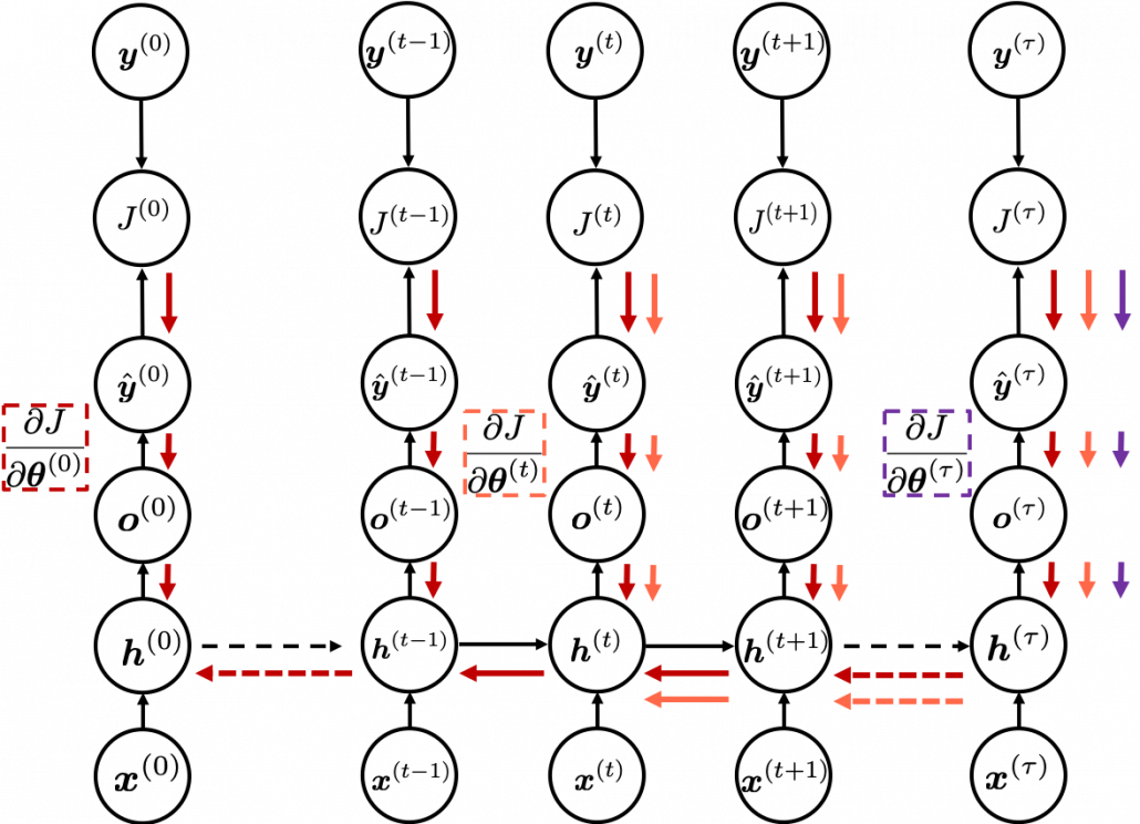
 are correct notations, because
  are values of neurons after forward propagation. They depend on time steps, and these are very values which I have been calling “errors.” That is why parameters do not depend on time steps, whereas errors depend on time steps.
 . With this gradient
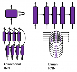

 , which most people would have seen in compulsory education, is a part of mapping. If you get a value x, you get a value y corresponding to the x.