How to make a toy English-German translator with multi-head attention heat maps: the overall architecture of Transformer
If you have been patient enough to read the former articles of this article series Instructions on Transformer for people outside NLP field, but with examples of NLP, you should have already learned a great deal of Transformer model, and I hope you gained a solid foundation of learning theoretical sides on this algorithm.
This article is going to focus more on practical implementation of a transformer model. We use codes in the Tensorflow official tutorial. They are maintained well by Google, and I think it is the best practice to use widely known codes.
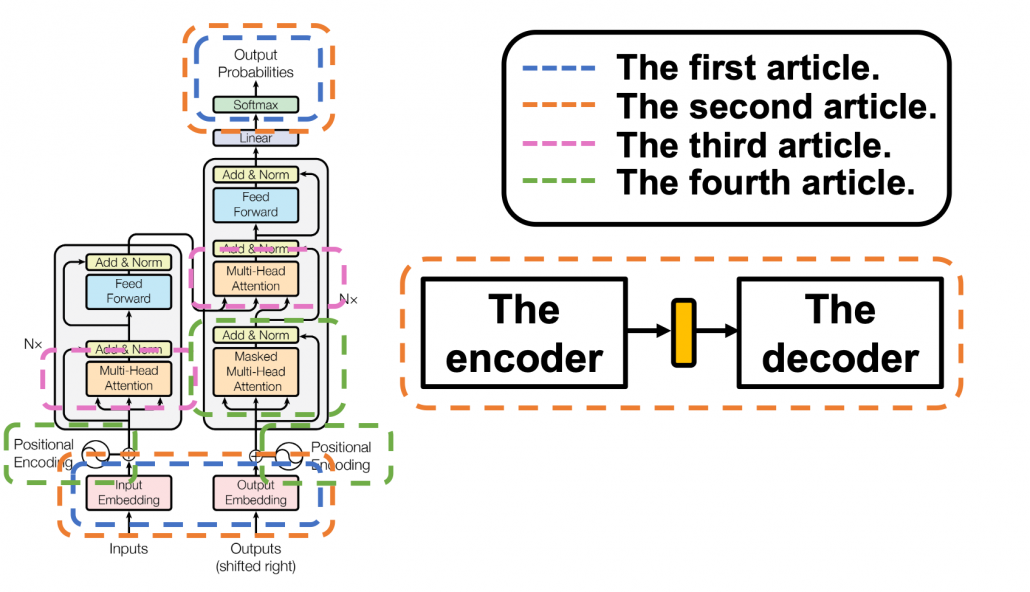
The figure below shows what I have explained in the articles so far. Depending on your level of understanding, you can go back to my former articles. If you are familiar with NLP with deep learning, you can start with the third article.
1 The datasets
I think this article series appears to be on NLP, and I do believe that learning Transformer through NLP examples is very effective. But I cannot delve into effective techniques of processing corpus in each language. Thus we are going to use a library named BPEmb. This library enables you to encode any sentences in various languages into lists of integers. And conversely you can decode lists of integers to the language. Thanks to this library, we do not have to do simplification of alphabets, such as getting rid of Umlaut.
*Actually, I am studying in computer vision field, so my codes would look elementary to those in NLP fields.
The official Tensorflow tutorial makes a Portuguese-English translator, but in article we are going to make an English-German translator. Basically, only the codes below are my original. As I said, this is not an article on NLP, so all you have to know is that at every iteration you get a batch of (64, 41) sized tensor as the source sentences, and a batch of (64, 42) tensor as corresponding target sentences. 41, 42 are respectively the maximum lengths of the input or target sentences, and when input sentences are shorter than them, the rest positions are zero padded, as you can see in the codes below.
*If you just replace datasets and modules for encoding, you can make translators of other pairs of languages.
We are going to train a seq2seq-like Transformer model of converting those list of integers, thus a mapping from a vector to another vector. But each word, or integer is encoded as an embedding vector, so virtually the Transformer model is going to learn a mapping from sequence data to another sequence data. Let’s formulate this into a bit more mathematics-like way: when we get a pair of sequence data 
 and
and 
 , where
  , respectively from English and German corpus, then we learn a mapping
  .
.
*In this implementation the vocabulary sizes are both  . Thus
2 The whole architecture
This article series has covered most of components of Transformer model, but you might not understand how seq2seq-like models can be constructed with them. It is very effective to understand how transformer is constructed by actually reading or writing codes, and in this article we are finally going to construct the whole architecture of a Transforme translator, following the Tensorflow official tutorial. At the end of this article, you would be able to make a toy English-German translator.
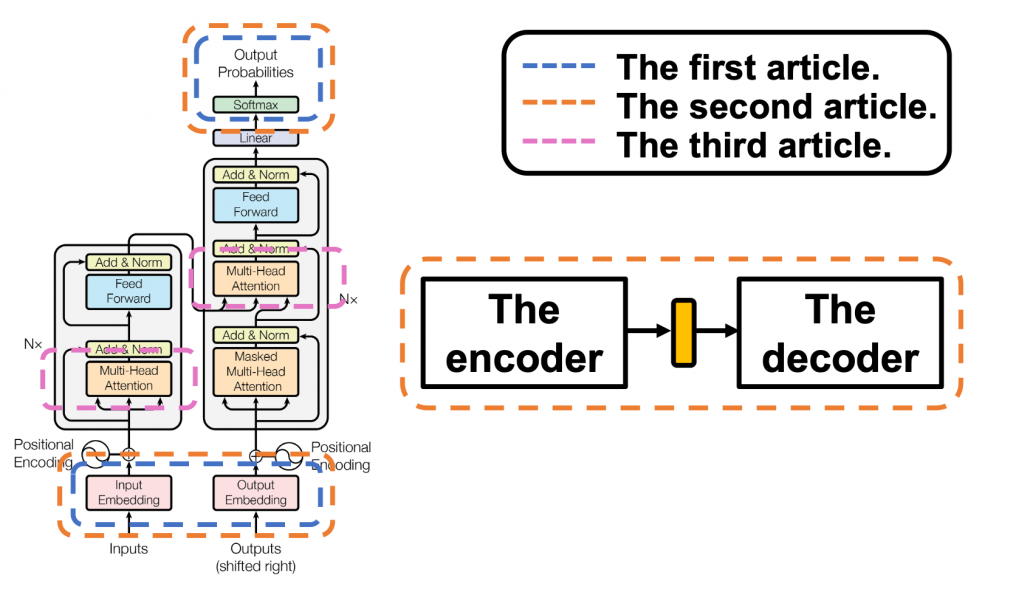
The implementation is mainly composed of 4 classes, EncoderLayer(), Encoder(), DecoderLayer(), and Decoder() class. The inclusion relations of the classes are displayed in the figure below.
![]()
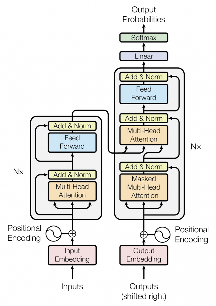
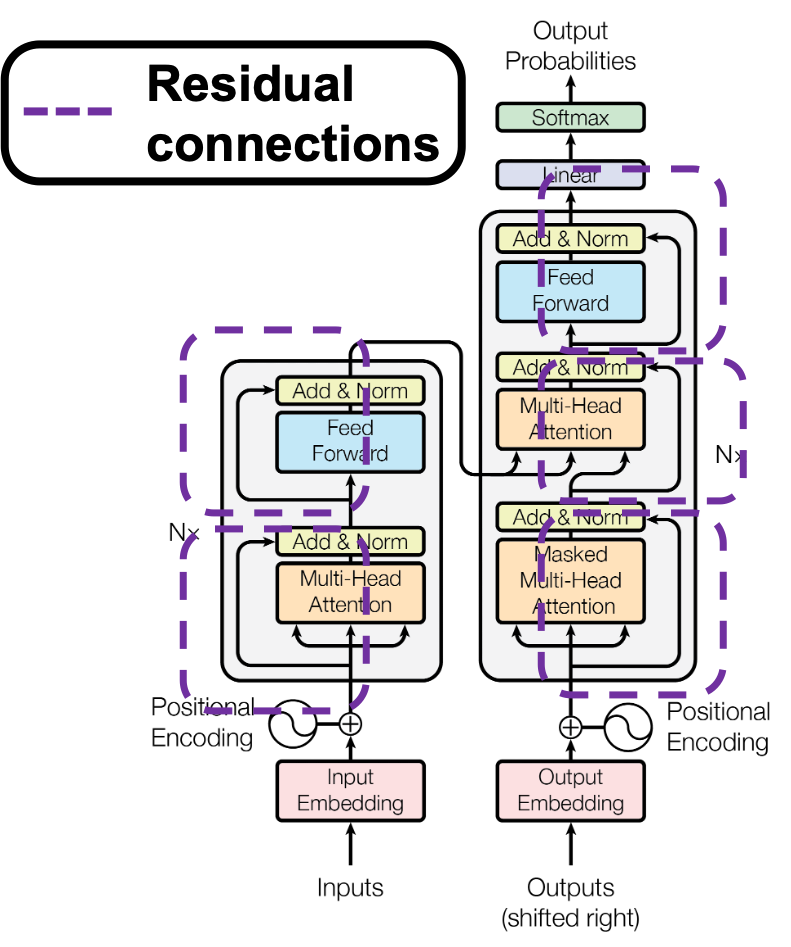
To be more exact in a seq2seq-like model with Transformer, the encoder and the decoder are connected like in the figure below. The encoder part keeps converting input sentences in the original language through  layers. The decoder part also keeps converting the inputs in the target languages, also through layers, but it receives the output of the final layer of the Encoder at every layer.
![]()
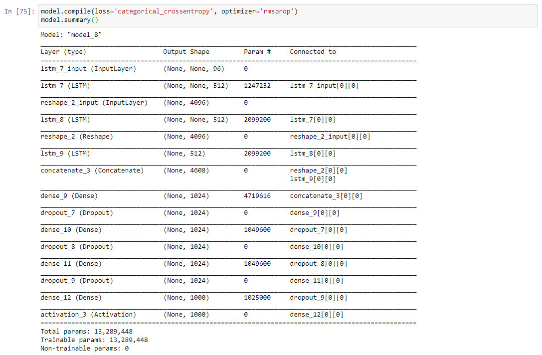
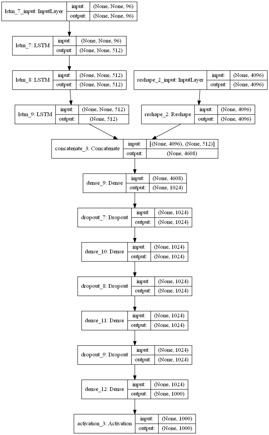
You can see how the Encoder() class and the Decoder() class are combined in Transformer in the codes below. If you have used Tensorflow or Pytorch to some extent, the codes below should not be that hard to read.
3 The encoder
*From now on “sentences” do not mean only the input tokens in natural language, but also the reweighted and concatenated “values,” which I repeatedly explained in explained in the former articles. By the end of this section, you will see that Transformer repeatedly converts sentences layer by layer, remaining the shape of the original sentence.
I have explained multi-head attention mechanism in the third article, precisely, and I explained positional encoding and masked multi-head attention in the last article. Thus if you have read them and have ever written some codes in Tensorflow or Pytorch, I think the codes of Transformer in the official Tensorflow tutorial is not so hard to read. What is more, you do not use CNNs or RNNs in this implementation. Basically all you need is linear transformations. First of all let’s see how the EncoderLayer() and the Encoder() classes are implemented in the codes below.
You might be confused what “Feed Forward” means in this article or the original paper on Transformer. The original paper says this layer is calculated as 
 . In short you stack two fully connected layers and activate it with a ReLU function. Let’s see how point_wise_feed_forward_network() function works in the implementation with some simple codes. As you can see from the number of parameters in each layer of the position wise feed forward neural network, the network does not depend on the length of the sentences.
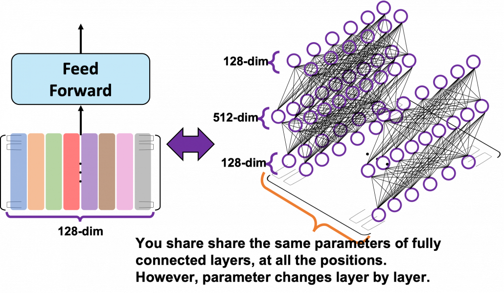
From the number of parameters of the position-wise feed forward neural networks, you can see that you share the same parameters over all the positions of the sentences. That means in the figure above, you use the same densely connected layers at all the positions, in single layer. But you also have to keep it in mind that parameters for position-wise feed-forward networks change from layer to layer. That is also true of “Layer” parts in Transformer model, including the output part of the decoder: there are no learnable parameters which cover over different positions of tokens. These facts lead to one very important feature of Transformer: the number of parameters does not depend on the length of input or target sentences. You can offset the influences of the length of sentences with multi-head attention mechanisms. Also in the decoder part, you can keep the shape of sentences, or reweighted values, layer by layer, which is expected to enhance calculation efficiency of Transformer models.
![]()
4, The decoder
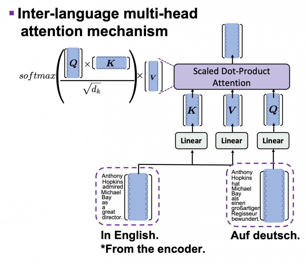
The structures of DecoderLayer() and the Decoder() classes are quite similar to those of EncoderLayer() and the Encoder() classes, so if you understand the last section, you would not find it hard to understand the codes below. What you have to care additionally in this section is inter-language multi-head attention mechanism. In the third article I was repeatedly explaining multi-head self attention mechanism, taking the input sentence “Anthony Hopkins admired Michael Bay as a great director.” as an example. However, as I explained in the second article, usually in attention mechanism, you compare sentences with the same meaning in two languages. Thus the decoder part of Transformer model has not only self-attention multi-head attention mechanism of the target sentence, but also an inter-language multi-head attention mechanism. That means, In case of translating from English to German, you compare the sentence “Anthony Hopkins hat Michael Bay als einen großartigen Regisseur bewundert.” with the sentence itself in masked multi-head attention mechanism (, just as I repeatedly explained in the third article). On the other hand, you compare “Anthony Hopkins hat Michael Bay als einen großartigen Regisseur bewundert.” with “Anthony Hopkins admired Michael Bay as a great director.” in the inter-language multi-head attention mechanism (, just as you can see in the figure above).
*The “inter-language multi-head attention mechanism” is my original way to call it.
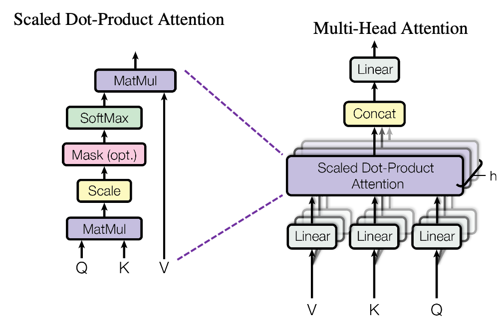
I briefly mentioned how you calculate the inter-language multi-head attention mechanism in the end of the third article, with some simple codes, but let’s see that again, with more straightforward figures. If you understand my explanation on multi-head attention mechanism in the third article, the inter-language multi-head attention mechanism is nothing difficult to understand. In the multi-head attention mechanism in encoder layers, “queries”, “keys”, and “values” come from the same sentence in English, but in case of inter-language one, only “keys” and “values” come from the original sentence, and “queries” come from the target sentence. You compare “queries” in German with the “keys” in the original sentence in English, and you re-weight the sentence in English. You use the re-weighted English sentence in the decoder part, and you do not need look-ahead mask in this inter-language multi-head attention mechanism.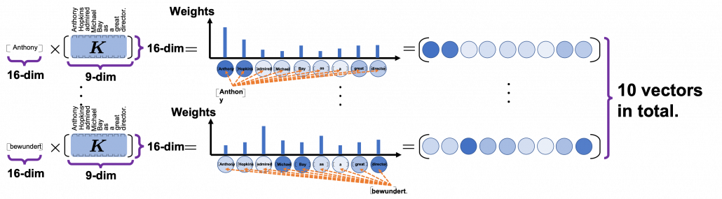
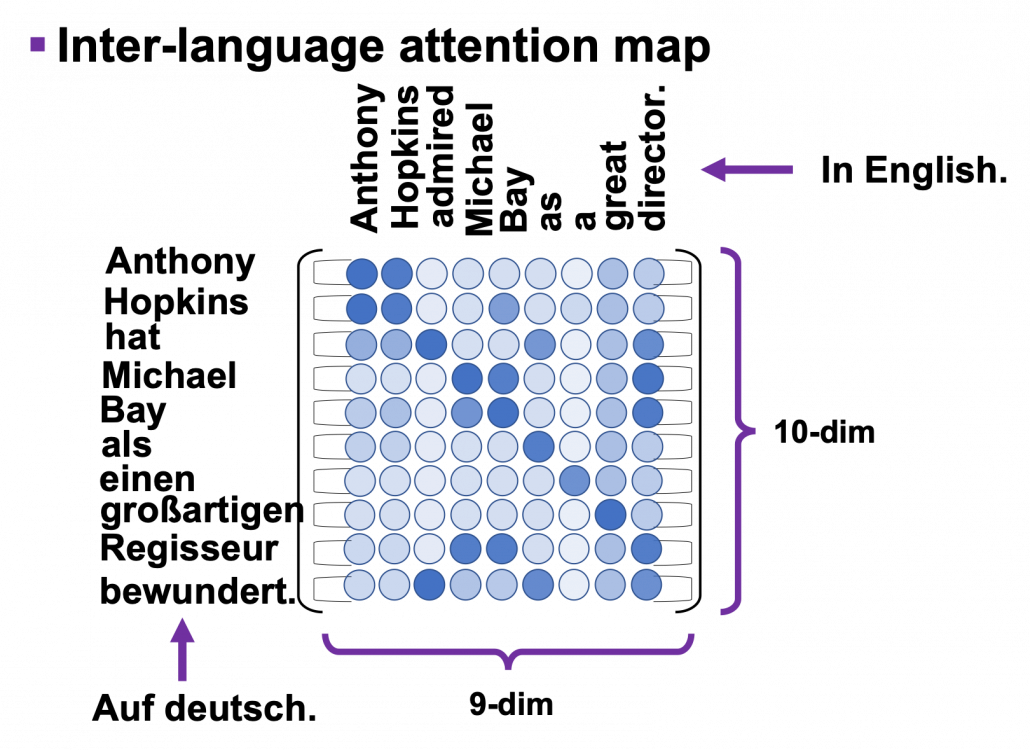
Just as well as multi-head self-attention, you can calculate inter-language multi-head attention mechanism as follows:  . In the example above, the resulting multi-head attention map is a
  matrix like in the figure below.
Once you keep the points above in you mind, the implementation of the decoder part should not be that hard.
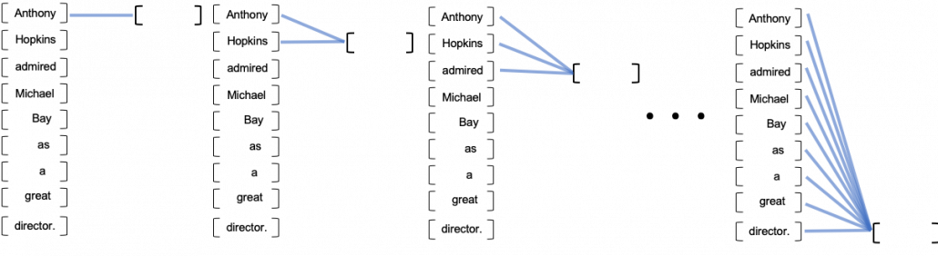
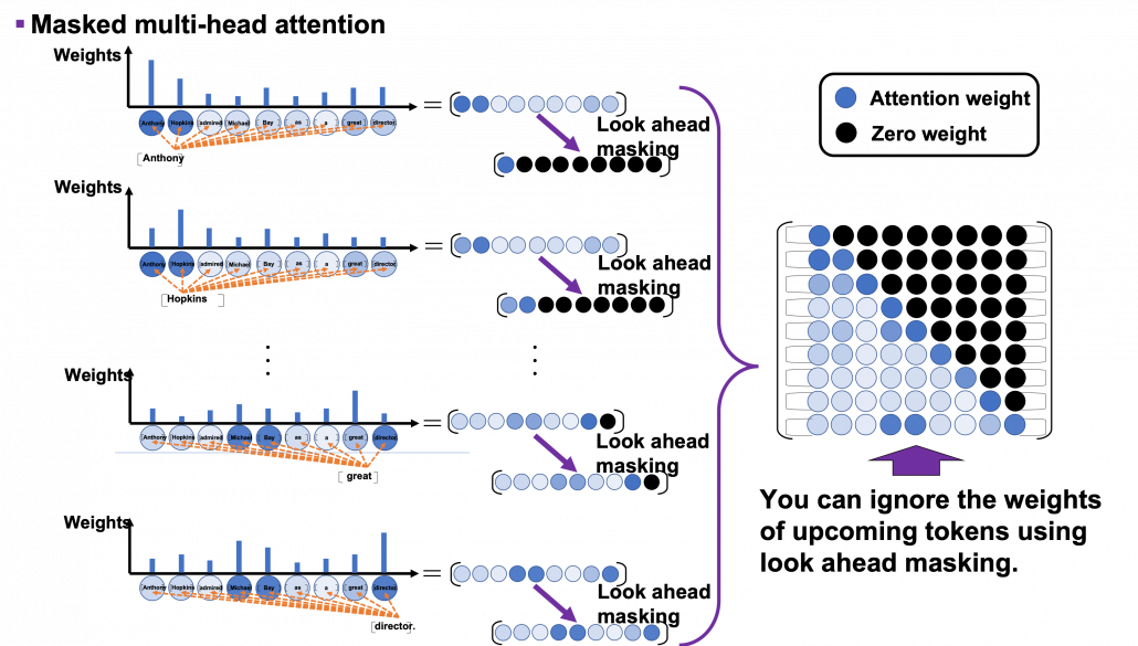
5 Masking tokens in practice
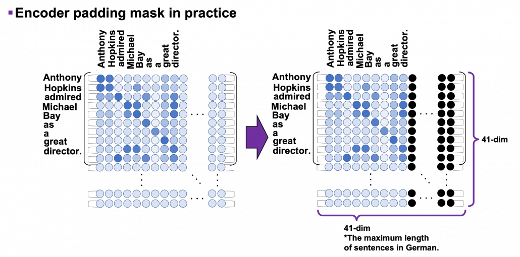
I explained masked-multi-head attention mechanism in the last article, and the ideas itself is not so difficult. However in practice this is implemented in a little tricky way. You might have realized that the size of input matrices is fixed so that it fits the longest sentence. That means, when the maximum length of the input sentences is 41, even if the sentences in a batch have less than 41 tokens, you sample (64, 41) sized tensor as a batch every time (The 64 is a batch size). Let “Anthony Hopkins admired Michael Bay as a great director.”, which has 9 tokens in total, be an input. We have been considering calculating (9, 9) sized attention maps or (10, 9) sized attention maps, but in practice you use (41, 41) or (42, 41) sized ones. When it comes to calculating self attentions in the encoder part, you zero pad self attention maps with encoder padding masks, like in the figure below. The black dots denote the zero valued elements.
As you can see in the codes below, encode padding masks are quite simple. You just multiply the padding masks with -1e9 and add them to attention maps and apply a softmax function. Thereby you can zero-pad the columns in the positions/columns where you added -1e9 to.
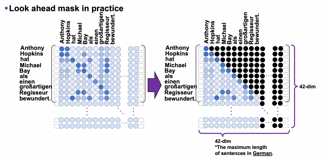
I explained look ahead mask in the last article, and in practice you combine normal padding masks and look ahead masks like in the figure below. You can see that you can compare each token with only its previous tokens. For example you can compare “als” only with “Anthony”, “Hopkins”, “hat”, “Michael”, “Bay”, “als”, not with “einen”, “großartigen”, “Regisseur” or “bewundert.”
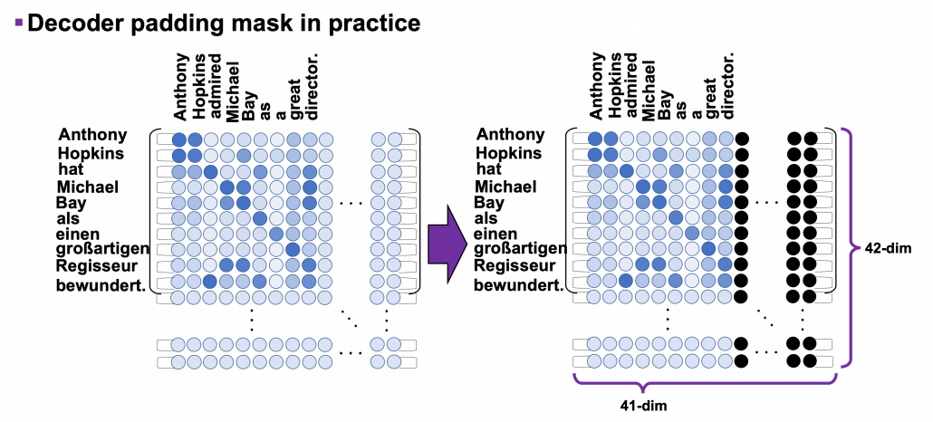
Decoder padding masks are almost the same as encoder one. You have to keep it in mind that you zero pad positions which surpassed the length of the source input sentence.
6 Decoding process
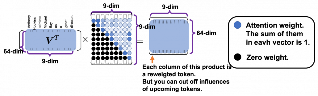
In the last section we have seen that we can zero-pad columns, but still the rows are redundant. However I guess that is not a big problem because you decode the final output in the direction of the rows of attention maps. Once you decode <end> token, you stop decoding. The redundant rows would not affect the decoding anymore.
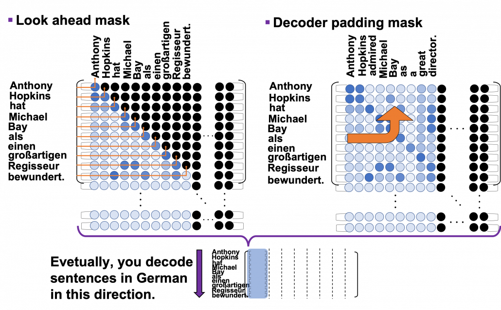
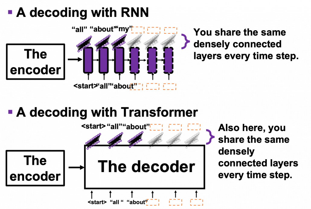
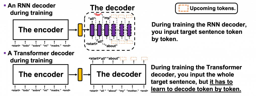
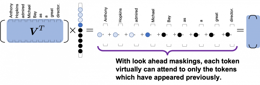
This decoding process is similar to that of seq2seq models with RNNs, and that is why you need to hide future tokens in the self-multi-head attention mechanism in the decoder. You share the same densely connected layers followed by a softmax function, at all the time steps of decoding. Transformer has to learn how to decode only based on the words which have appeared so far.
According to the original paper, “We also modify the self-attention sub-layer in the decoder stack to prevent positions from attending to subsequent positions. This masking, combined with fact that the output embeddings are offset by one position, ensures that the predictions for position  can depend only on the known outputs at positions less than .” After these explanations, I think you understand the part more clearly.
The codes blow is for the decoding part. You can see that you first start decoding an output sentence with a sentence composed of only <start>, and you decide which word to decoded, step by step.
*It easy to imagine that this decoding procedure is not the best. In reality you have to consider some possibilities of decoding, and you can do that with beam search decoding.
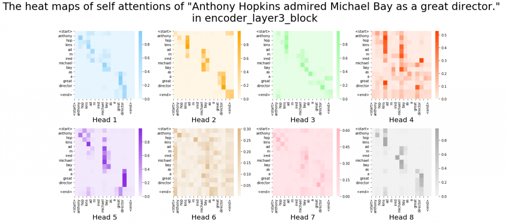
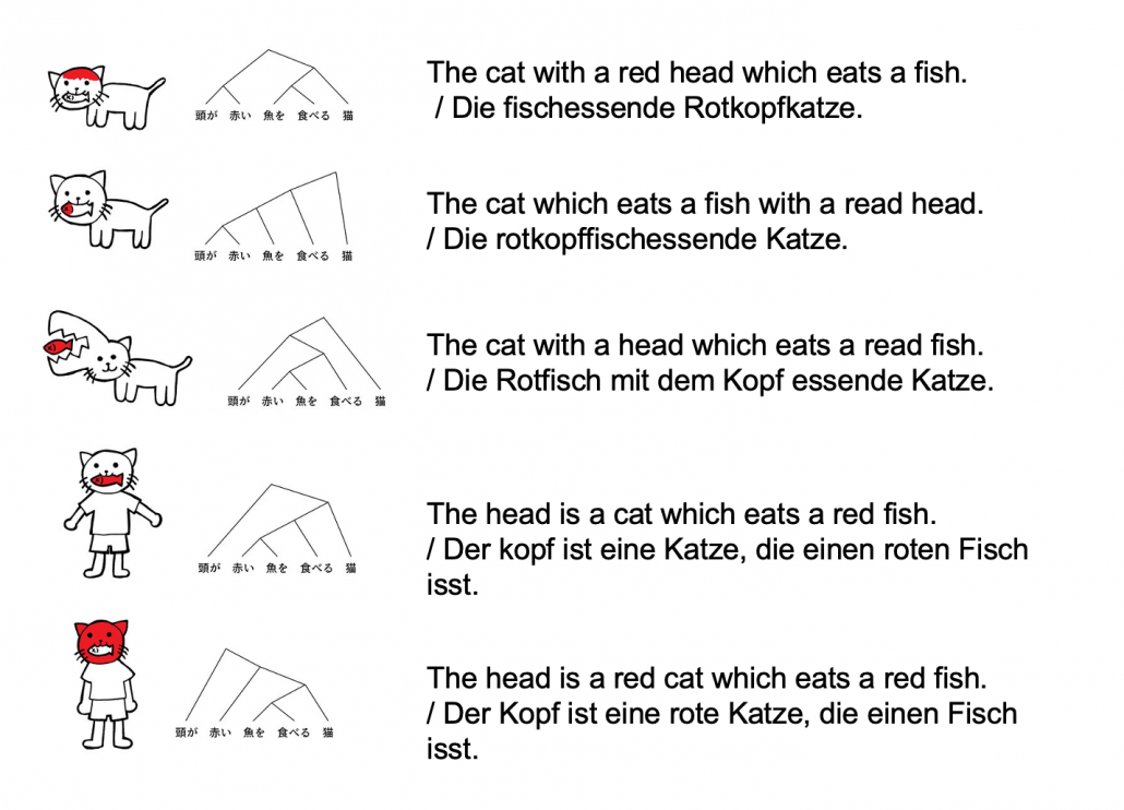
After training this English-German translator for 30 epochs you can translate relatively simple English sentences into German. I displayed some results below, with heat maps of multi-head attention. Each colored attention maps corresponds to each head of multi-head attention. The examples below are all from the fourth (last) layer, but you can visualize maps in any layers. When it comes to look ahead attention, naturally only the lower triangular part of the maps is activated.
This article series has not covered some important topics machine translation, for example how to calculate translation errors. Actually there are many other fascinating topics related to machine translation. For example beam search decoding, which consider some decoding possibilities, or other topics like how to handle proper nouns such as “Anthony” or “Hopkins.” But this article series is not on NLP. I hope you could effectively learn the architecture of Transformer model with examples of languages so far. And also I have not explained some details of training the network, but I will not cover that because I think that depends on tasks. The next article is going to be the last one of this series, and I hope you can see how Transformer is applied in computer vision fields, in a more “linguistic” manner.
But anyway we have finally made it. In this article series we have seen that one of the earliest computers was invented to break Enigma. And today we can quickly make a more or less accurate translator on our desk. With Transformer models, you can even translate deadly funny jokes into German.
*You can train a translator with this code.
*After training a translator, you can translate English sentences into German with this code.
[References]
[1] Ashish Vaswani, Noam Shazeer, Niki Parmar, Jakob Uszkoreit, Llion Jones, Aidan N. Gomez, Lukasz Kaiser, Illia Polosukhin, “Attention Is All You Need” (2017)
[2] “Transformer model for language understanding,” Tensorflow Core
https://www.tensorflow.org/overview
[3] Jay Alammar, “The Illustrated Transformer,”
http://jalammar.github.io/illustrated-transformer/
[4] “Stanford CS224N: NLP with Deep Learning | Winter 2019 | Lecture 14 – Transformers and Self-Attention,” stanfordonline, (2019)
https://www.youtube.com/watch?v=5vcj8kSwBCY
[5]Tsuboi Yuuta, Unno Yuuya, Suzuki Jun, “Machine Learning Professional Series: Natural Language Processing with Deep Learning,” (2017), pp. 91-94
坪井祐太、海野裕也、鈴木潤 著, 「機械学習プロフェッショナルシリーズ 深層学習による自然言語処理」, (2017), pp. 191-193
* I make study materials on machine learning, sponsored by DATANOMIQ. I do my best to make my content as straightforward but as precise as possible. I include all of my reference sources. If you notice any mistakes in my materials, including grammatical errors, please let me know (email: yasuto.tamura@datanomiq.de). And if you have any advice for making my materials more understandable to learners, I would appreciate hearing it.
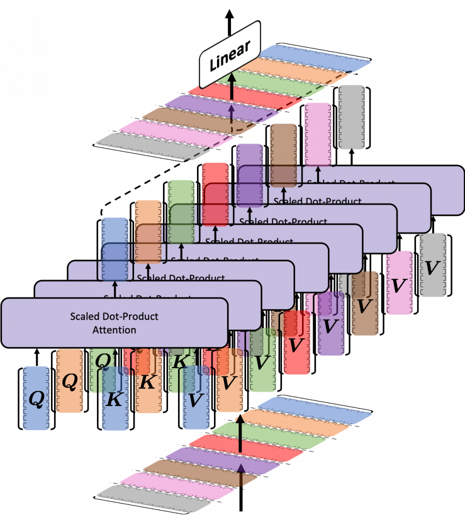
 matrix. You first split each token into
  dimensional, 8 vectors in total, as I colored in the figure below. In other words, the input matrix is divided into 8 colored chunks, which are all
  matrices, but each colored matrix expresses the same sentence. And you calculate self-attentions of the input sentence independently in the 8 heads, and you reweight the “values” according to the attentions/weights. After this, you stack the sum of the reweighted “values” in each colored head, and you concatenate the stacked tokens of each colored head. The size of each colored chunk does not change even after reweighting the tokens. According to Ashish Vaswani, who invented Transformer model, each head compare “queries” and “keys” on each standard. If the a Transformer model has 4 layers with 8-head multi-head attention , at least its encoder has
  heads, so the encoder learn the relations of tokens of the input on 32 different standards.
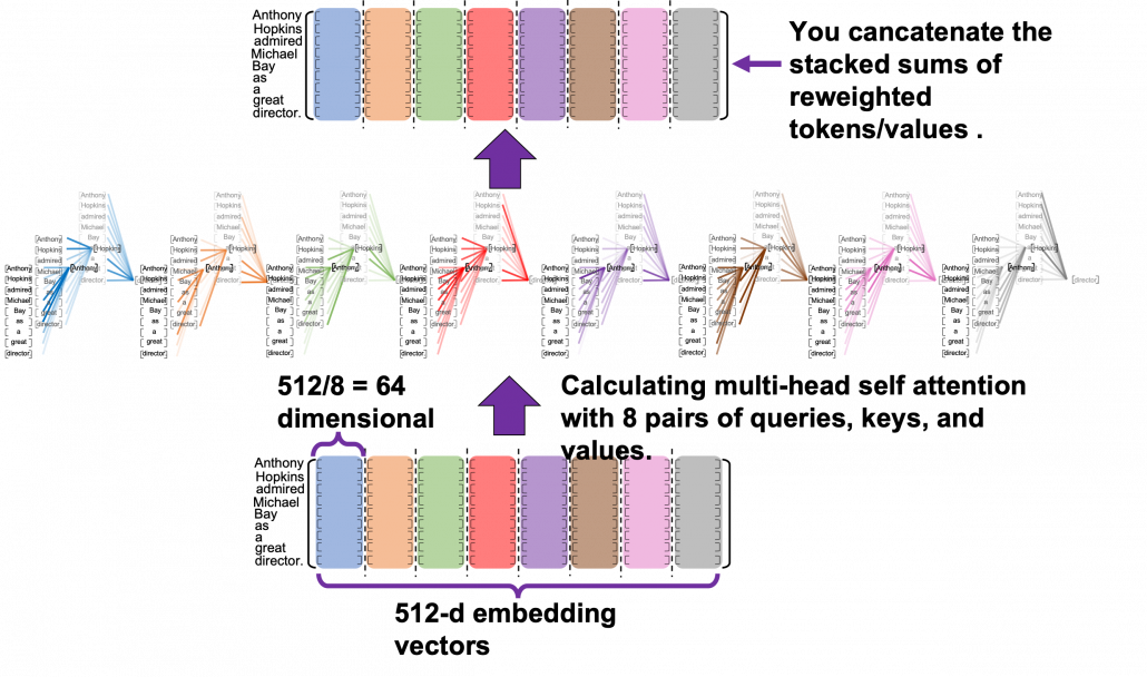
![[ \cdots ]](https://data-science-blog.com/en/wp-content/ql-cache/quicklatex.com-a935a6ae352397cdde28cd5115cc275a_l3.png "Rendered by QuickLaTeX.com") denotes a token, which is usually an embedding vector in practice.
denotes a token, which is usually an embedding vector in practice.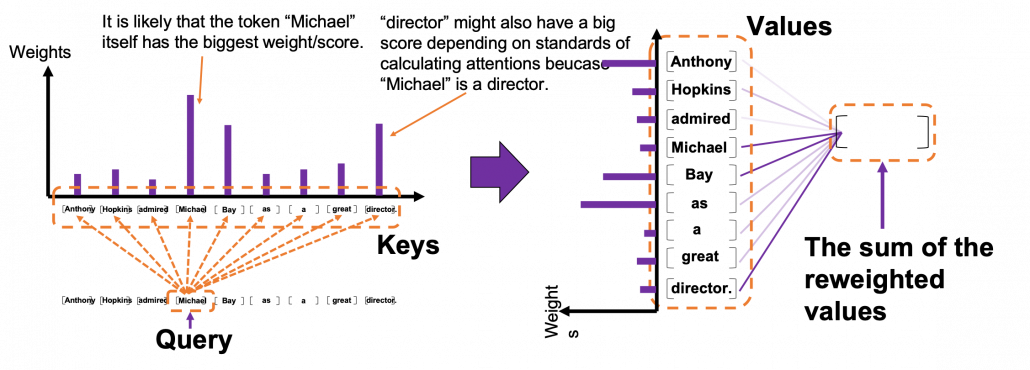 *I have been repeating the phrase “reweighting ‘values’ with attentions,” but you in practice calculate the sum of those reweighted “values.”
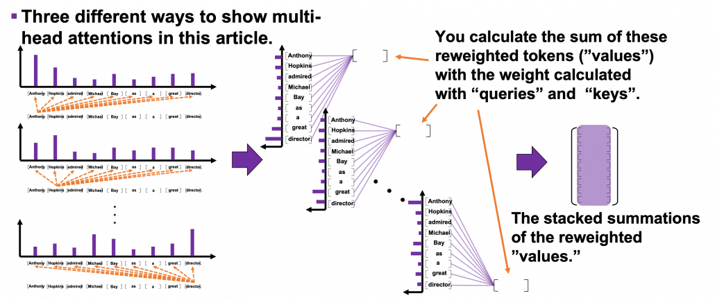

 . Let’s take an example of calculating a scaled dot-product in the blue head.
 , which are “queries”, “keys”, and “values” respectively.
 by
by  in the formula. According to the original paper, it is known that re-scaling
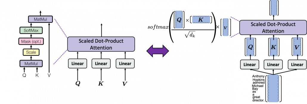
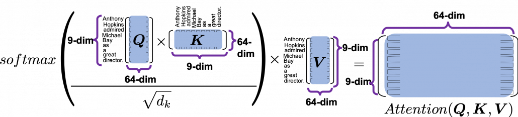
 , and the resulting
  matrix is a kind a heat map of self-attentions.
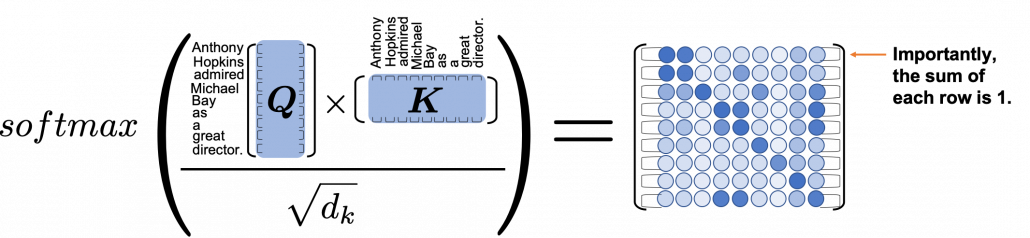
 and regularizing them with a softmax function, you stack those vectors, and the stacked vectors is the heat map of attentions.
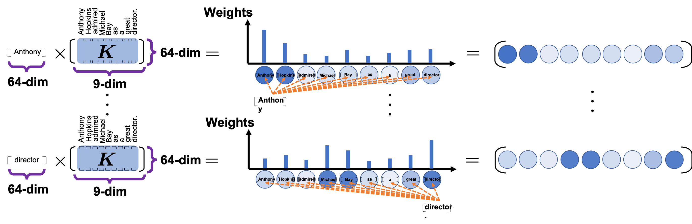
 . This also should be easy to understand if you know basics of linear algebra.
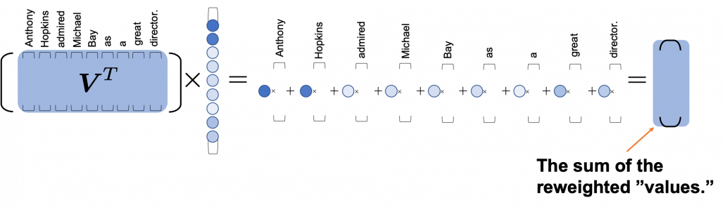
 tokens, basically you have to wait for
  the RNN cell retains the information at the time step
  only via recurrent connections. In this way you cannot attend to tokens in the earlier time steps, and this is obviously far from how we compare tokens in a sentence. You can bring information backward by bidirectional connection s in RNN models, but that all the more deteriorate parallelization of the model. And possessing information via recurrent connections, like a telephone game, potentially has risks of vanishing gradient problems. Gated RNN, such as LSTM or GRU mitigate the problems by a lot of nonlinear functions, but that adds to computational costs. If you understand multi-head attention mechanism, I think you can see that Transformer solves those problems.
 , but if you naively give the term
 ![[0, 1]](https://data-science-blog.com/en/wp-content/ql-cache/quicklatex.com-caffaae885a1287e3dfc31bfb1cd0694_l3.png "Rendered by QuickLaTeX.com") . With this approach, however, the resolution of encodings can vary depending on the length of the input sequence data. Thus these naive approaches do not meet the requirements above, and I guess even conventional RNN-based models were not so successful in these points.
. With this approach, however, the resolution of encodings can vary depending on the length of the input sequence data. Thus these naive approaches do not meet the requirements above, and I guess even conventional RNN-based models were not so successful in these points. ,
,  , where
  .
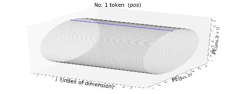
.  is the dimension of word embedding. The heat map below is the most typical type of visualization of positional encoding you would see everywhere, and in this case
  , and
, and  is discrete number which varies from
  to
to  , thus the heat map blow is equal to a
  matrix, whose elements are from
  to
to  . Each row of the graph corresponds to one token, and you can see that lower dimensional part is constantly changing like waves. Also it is quite easy to encode an input with this positional encoding: assume that you have a matrix of an input sentence composed of 50 tokens, each of which is a 256 dimensional vector, then all you have to do is just adding the heat map below to the matrix.
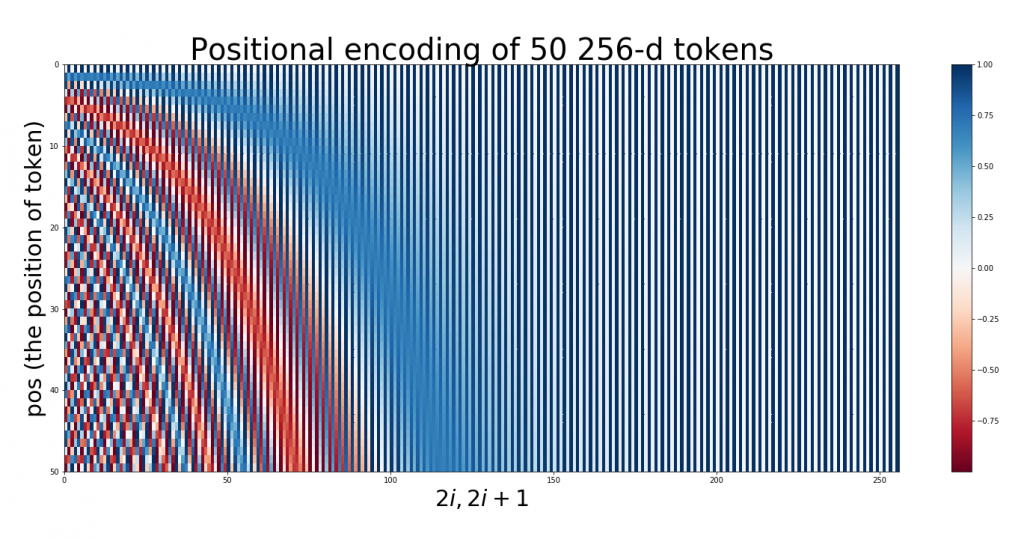

 .
. pairs of circles rather than
 . If you constantly change the value
  rotates clockwise on the unit circle in the figure below.
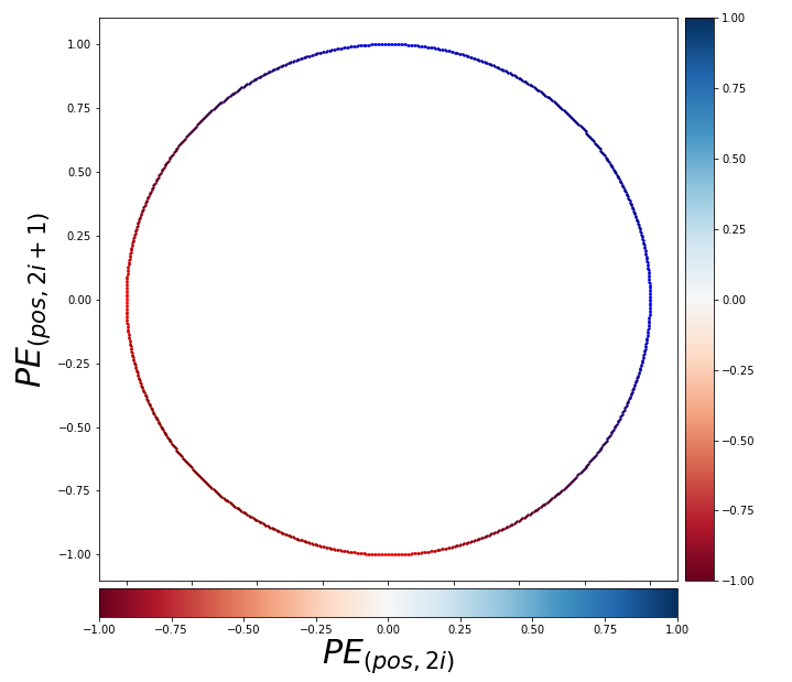
 ,
,  can be represented as a linear function of
  .” For each circle at any depth, I mean for any

 , where
  . Also the shift from “Bay” to “great” has the same rotation.
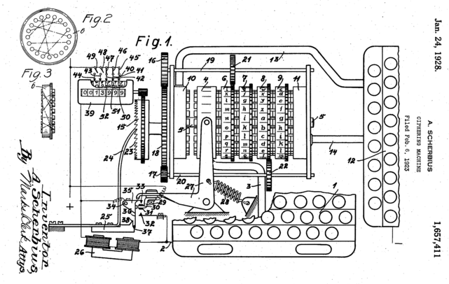
 ', fontsize=30)
plt.colorbar()
plt.title("Positional encoding of 50 256-d tokens", fontsize=40)
plt.savefig("positional_encoding_heat_map.png")
plt.show()
', fontsize=30)
plt.colorbar()
plt.title("Positional encoding of 50 256-d tokens", fontsize=40)
plt.savefig("positional_encoding_heat_map.png")
plt.show()
 ', fontsize=40)
ax.set_zlabel(r'
', fontsize=40)
ax.set_zlabel(r' ', fontsize=40)
ax.set_xticks(np.arange(0, d_model//2, 10))
plt.subplots_adjust(left=0, right=1, bottom=0, top=1)
#plt.savefig('./positional_encoding_gif/{}.png'.format(j+1))
plt.show()
', fontsize=40)
ax.set_xticks(np.arange(0, d_model//2, 10))
plt.subplots_adjust(left=0, right=1, bottom=0, top=1)
#plt.savefig('./positional_encoding_gif/{}.png'.format(j+1))
plt.show()
 , and it includes words from “a”, “ablation”, “actually” to “zombie”, “?”, “!”
 , where only the No. i element is
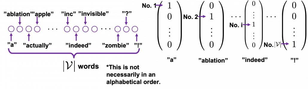
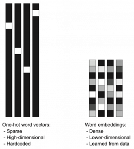
 dimensional vector, whose dimension is fewer than the vocabulary size
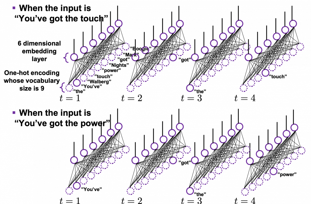
 . When the inputs are “You’ve got the touch” or “You’ve got the power” , you put the one-hot vector corresponding to “You’ve”, “got”, “the”, “touch” or “You’ve”, “got”, “the”, “power” sequentially every time step
  .
.
 ,
,  .
. , a list of vectors. The vectors are usually embedding vectors, and the
  , where
  denote “You’ve”, “got”, “the”, “power”, “.” respectively. In this case
  .
. usually includes two tokens
  and
and  at the beginning and the end of the sentence. They mean “Beginning Of Sentence” and “End Of Sentence” respectively. Thus in many cases
  .
.  and
and  are also both vectors, at least in the Tensorflow tutorial.
 is the probability of incidence of the sentence. But it is easy to imagine that it would be very hard to directly calculate how likely the sentence
  as a product of the probability of incidence or a certain word, given all the words so far. When you’ve got the words
  so far, the probability of the incidence of
  , given the context is
  .
.  is a probability of the the sentence
  , and the probability of
  can be decomposed this way:
 .
.

 .
.


 be
be  be
be ![P(\boldsymbol{x}^{(t+1)}|\boldsymbol{X}_{[0, t]})](https://data-science-blog.com/en/wp-content/ql-cache/quicklatex.com-9b85b225f0635a7627a99481018f6166_l3.png "Rendered by QuickLaTeX.com") be
be  , then
 ![P(\boldsymbol{X}) = P(\boldsymbol{x}^{(0)})\prod_{t=0}^{\tau}{P(\boldsymbol{x}^{(t+1)}|\boldsymbol{X}_{[0, t]})}](https://data-science-blog.com/en/wp-content/ql-cache/quicklatex.com-59e2d215f0fea11ec20386dfef220a30_l3.png "Rendered by QuickLaTeX.com") . Language models calculate which words to come sequentially in this way.
. Language models calculate which words to come sequentially in this way.


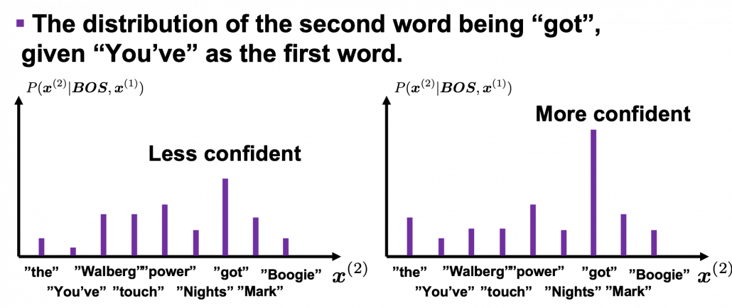
![P(\boldsymbol{x}^{(0)})\prod_{t=0}^{4}{P(\boldsymbol{x}^{(t+1)}|\boldsymbol{X}_{[0, t]})}](https://data-science-blog.com/en/wp-content/ql-cache/quicklatex.com-4d263b8554a322d3ab8a8841552bc75b_l3.png "Rendered by QuickLaTeX.com") . Given a context
. Given a context  is
is  . In the figure below, the distribution at the left side is less confident because probabilities do not spread widely, on the other hand the one at the right side is more confident that next word is “got” because the distribution concentrates on “got”.
 is
is 

 .
.


 gets higher. Thus


 gets lower, where usually
  or
or  .
. , which is composed of
  sentences in total. Each sentence
![(\boldsymbol{x}^{(0)})\prod_{t=0}^{\tau ^{(n)}}{P(\boldsymbol{x}_{n}^{(t+1)}|\boldsymbol{X}_{n, [0, t]})}](https://data-science-blog.com/en/wp-content/ql-cache/quicklatex.com-ccc74ac2aee4f90a6b035dcfd2632927_l3.png "Rendered by QuickLaTeX.com") has
has  tokens in total excluding
  . And let
  , where
 ![z = \frac{-1}{|\mathcal{V}|}\sum_{n=1}^{|\mathcal{D}|}{\sum_{t=0}^{\tau ^{(n)}}{log_{b}P(\boldsymbol{x}_{n}^{(t+1)}|\boldsymbol{X}_{n, [0, t]})}](https://data-science-blog.com/en/wp-content/ql-cache/quicklatex.com-c1ccb76fcad455ad635fc1ec8b2f6f81_l3.png "Rendered by QuickLaTeX.com") . The
. The  is usually
  or
or  .
. is vocabulary {“the”, “You’ve”, “Walberg”, “touch”, “power”, “Nights”, “got”, “Mark”, “Boogie”}. Also assume that the evaluation data set for perplexity of a language model is
  , where
 . In this case
 . I have already showed you how to calculate the perplexity of the sentence “You’ve got the touch.” above. You just need to do a similar thing on another sentence “You’ve got the power”, and then you can get the perplexity of the language model.