How Do Various Actor-Critic Based Deep Reinforcement Learning Algorithms Perform on Stock Trading?
Deep Reinforcement Learning for Automated Stock Trading: An Ensemble Strategy
Abstract
Deep Reinforcement Learning (DRL) is a blooming field famous for addressing a wide scope of complex decision-making tasks. This article would introduce and summarize the paper “Deep Reinforcement Learning for Automated Stock Trading: An Ensemble Strategy”, and discuss how these actor-critic based DRL learning algorithms, Proximal Policy Optimization (PPO), Advantage Actor Critic (A2C), and Deep Deterministic Policy Gradient (DDPG), act to accomplish automated stock trading by boosting investment return.
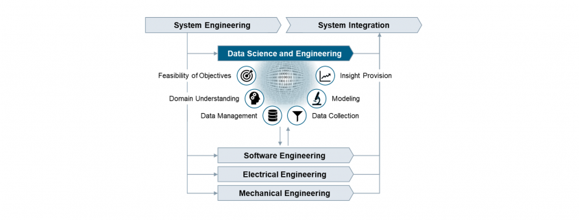
1 Motivation and Related Technology
It has long been challenging to design a comprehensive strategy for capital allocation optimization in a complex and dynamic stock market. With development of Artificial Intelligence, machine learning coupled with fundamentals analysis and alternative data has been in trend and provides better performance than conventional methodologies. Reinforcement Learning (RL) as a branch of it, is able to learn from interactions with environment, during which the agent continuously absorbs information, takes actions, and learns to improve its policy regarding rewards or losses obtained. On top of that, DRL utilizes neural networks as function approximators to approximate the Q-value (the expected reward of each action) in RL, which in return adjusts RL for large-scale data learning.
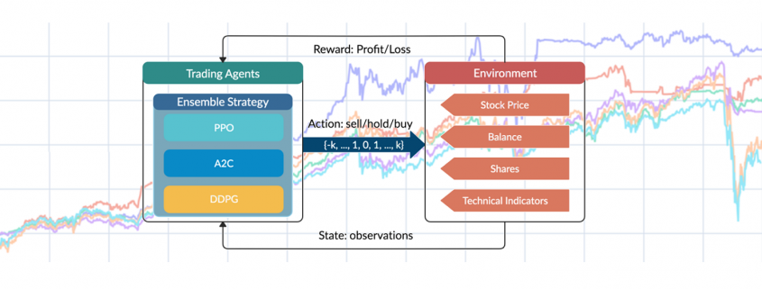
In DRL, the critic-only approach is capable for solving discrete action space problems, calculating Q-value to learn the optimal action-selection policy. On the other side, the actor-only approach, used in continuous action space environments, directly learns the optimal policy itself. Combining both, the actor-critic algorithm simultaneously updates the actor network representing the policy, and critic network representing the value function. The critic estimates the value function, while the actor updates the policy guided by the critic with policy gradients.
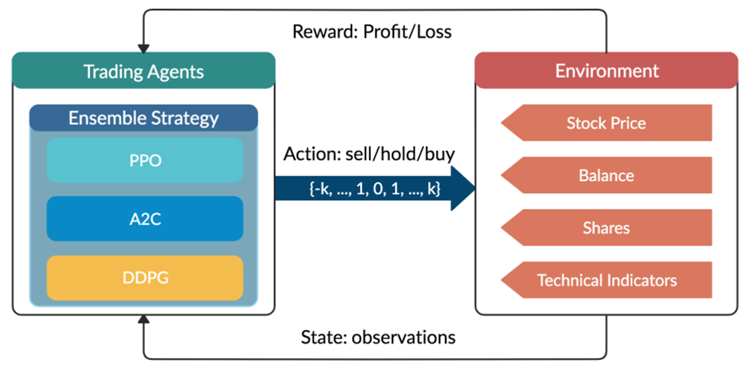
Figure 1: Overview of reinforcement learning-based stock theory.
2 Mathematical Modeling
2.1 Stock Trading Simulation
Given the stochastic nature of stock market, the trading process is modeled as a Markov Decision Process (MDP) as follows:
- State s = [p, h, b]: a vector describing the current state of the portfolio consists of D stocks, includes stock prices vector p, the stock shares vector h, and the remaining balance b.
- Action a: a vector of actions which are selling, buying, or holding (Fig.2), resulting in decreasing, increasing, and no change of shares h, respectively. The number of shares been transacted is recorded as k.
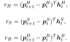
- Reward r(s, a, s’): the reward of taking action a at state s and arriving at the new state s’.
- Policy π(s): the trading strategy at state s, which is the probability distribution of actions.
- Q-value : the expected reward of taking action a at state s following policy π.
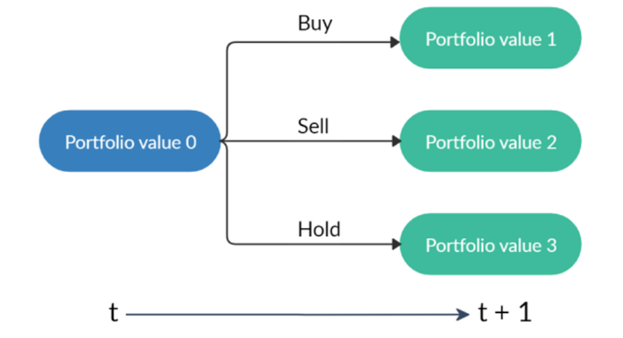
A starting portfolio value with three actions result in three possible portfolios. Note that “hold” may lead to different portfolio values due to the changing stock prices.
Besides, several assumptions and constraints are proposed for practice:
- Market liquidity: the orders are rapidly executed at close prices.
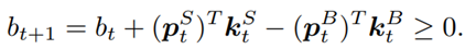
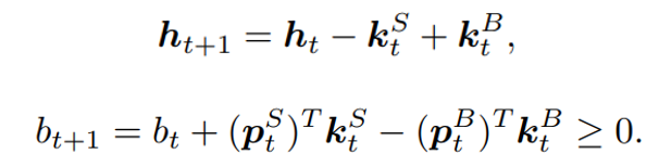
- Nonnegative balance: the balance at time t+1 after taking actions at t, equals to the original balance plus the proceeds of selling minus the spendings of buying:
- Transaction cost: assume the transaction costs to be 0.1% of the value of each trade:

- Risk-aversion: to control the risk of stock market crash caused by major emergencies, the financial turbulence index that measures extreme asset price movements is introduced:

where denotes the stock returns, µ and Σ are respectively the average and covariance of historical returns. When exceeds a threshold, buying will be halted and the agent sells all shares. Trading will be resumed once returns to normal level.
2.2 Trading Goal: Return Maximation
The goal is to design a trading strategy that raises agent’s total cumulative compensation given by the reward function:
![]()
and then considering the transition of the shares and the balance defined as:
the reward can be further decomposed:
![]()
where:
At inception, h and  are initialized to 0, while the policy π(s) is uniformly distributed among all actions. Afterwards, everything is updated through interacting with the stock market environment. By the Bellman Equation,
  is the expectation of the sum of direct reward
  and the future reqard
  at the next state discounted by a factor γ, resulting in the state-action value function:
![]()
2.3 Environment for Multiple Stocks
OpenAI gym is used to implement the multiple stocks trading environment and to train the agent.
- State Space: a vector
![[b_t, p_t, h_t, M_t, R_t, C_t, X_t]](https://data-science-blog.com/en/wp-content/ql-cache/quicklatex.com-0fbdf800e4e901e62bc4396f3815d15f_l3.png "Rendered by QuickLaTeX.com") storing information about
storing information about
 : Portfolio balance
 : Adjusted close prices
 : Shares owned of each stock
 : Moving Average Convergence Divergence
 : Relative Strength Index
 : Commodity Channel Index
 : Average Directional Index
 - Action Space: {−k, …, −1, 0, 1, …, k} for a single stock, whose elements representing the number of shares to buy or sell. The action space is then normalized to [−1, 1], since A2C and PPO are defined directly on a Gaussian distribution.
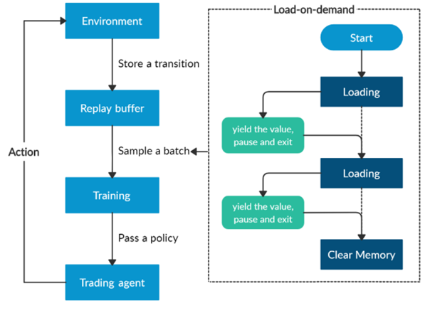
Overview of the load-on-demand technique.
Furthermore, a load-on-demand technique is applied for efficient use of memory as shown above.
- Algorithms Selection
This paper mainly uses the following three actor-critic algorithms:
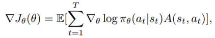
- A2C: uses parallel copies of the same agent to update gradients for different data samples, and a coordinator to pass the average gradients over all agents to a global network, which can update the actor and the critic network, with the objective function:
- where
 is the policy network, and
  is the advantage function to reduce the high variance of it:
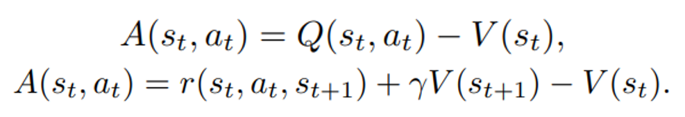
 is the value function of state
  , regardless of actions. DDPG: combines the frameworks of Q-learning and policy gradients and uses neural networks as function approximators; it learns directly from the observations through policy gradient and deterministically map states to actions. The Q-value is updated by:
 Critic network is then updated by minimizing the loss function:

- PPO: controls the policy gradient update to ensure that the new policy does not differ too much from the previous policy, with the estimated advantage function and a probability ratio:

The clipped surrogate objective function:
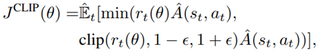
takes the minimum of the clipped and normal objective to restrict the policy update at each step and improve the stability of the policy.
An ensemble strategy is finally proposed to combine the three agents together to build a robust trading strategy. After training and testing the three agents concurrently, in the trading stage, the agent with the highest Sharpe ratio in one period will be automatically selected to use in the next period.
- Implementation: Training and Validation
The historical daily trading data comes from the 30 DJIA constituent stocks.
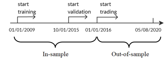
Stock data splitting in-sample and out-of-sample.
- In-sample training stage: data from 01/01/2009 – 09/30/2015 used to train 3 agents using PPO, A2C, and DDPG;
- In-sample validation stage: data from 10/01/2015 – 12/31/2015 used to validate the 3 agents by 5 metrics: cumulative return, annualized return, annualized volatility, Sharpe ratio, and max drawdown; tune key parameters like learning rate and number of episodes;
- Out-of-sample trading stage: unseen data from 01/01/2016 – 05/08/2020 to evaluate the profitability of algorithms while continuing training. In each quarter, the agent with the highest Sharpe ratio is selected to act in the next quarter, as shown below.
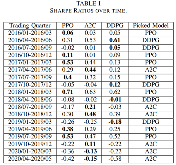
Table 1 – Sharpe Ratios over time.
- Results Analysis and Conclusion
From Table II and Fig.5, one can notice that PPO agent is good at following trend and performs well in chasing for returns, with the highest cumulative return 83.0% and annual return 15.0% among the three agents, indicating its appropriateness in a bullish market. A2C agent is more adaptive to handle risk, with the lowest annual volatility 10.4% and max drawdown −10.2%, suggesting its capability in a bearish market. DDPG generates the lowest return among the three, but works fine under risk, with lower annual volatility and max drawdown than PPO. Apparently all three agents outperform the two benchmarks.
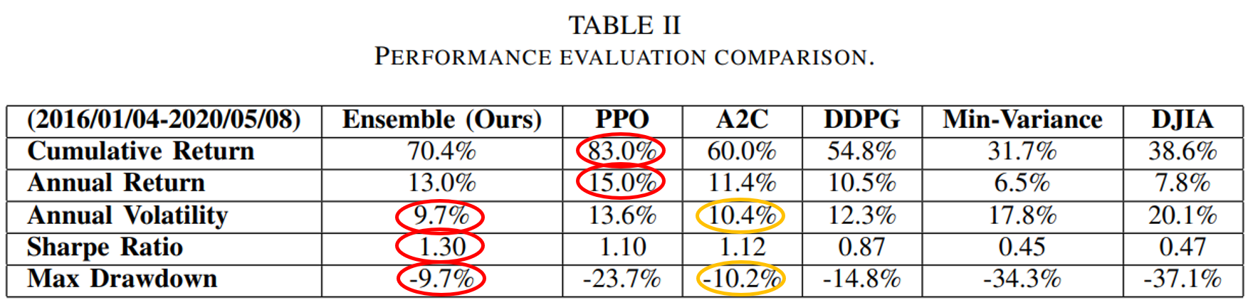
Table 2 – Performance Evaluation Comparison.

Moreover, it is obvious in Fig.6 that the ensemble strategy and the three agents act well during the 2020 stock market crash, when the agents successfully stops trading, thus cutting losses.
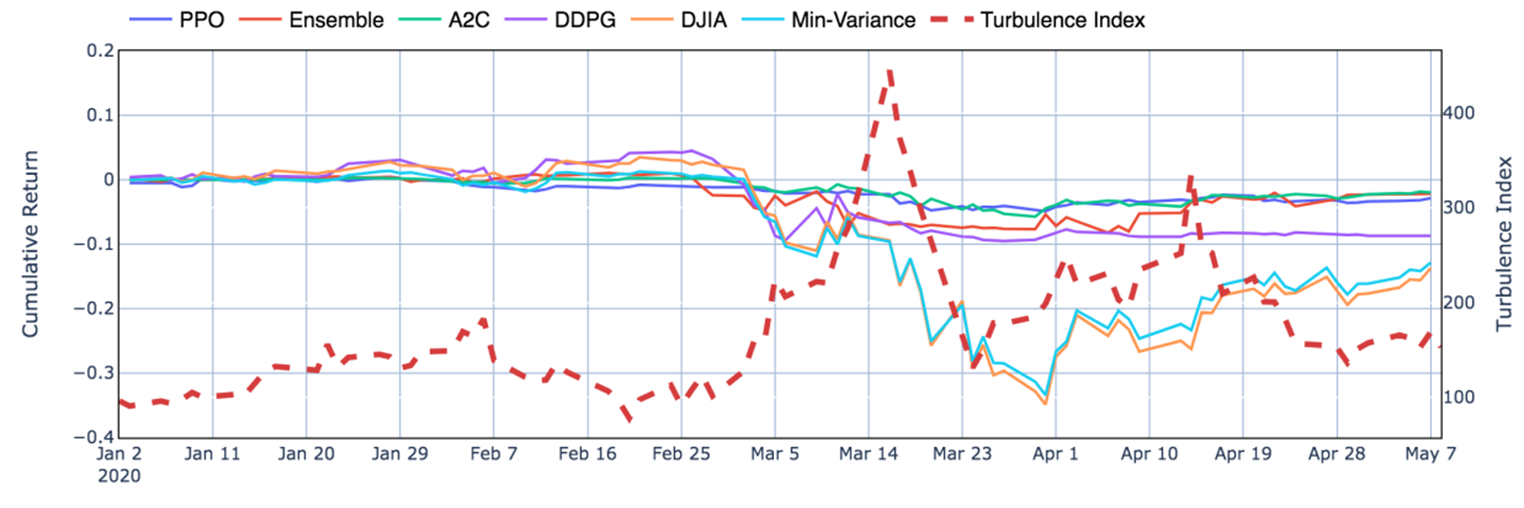
Performance during the stock market crash in the first quarter of 2020.
From the results, the ensemble strategy demonstrates satisfactory returns and lowest volatilities. Although its cumulative returns are lower than PPO, it has achieved the highest Sharpe ratio 1.30 among all strategies. It is reasonable that the ensemble strategy indeed performs better than the individual algorithms and baselines, since it works in a way each elemental algorithm is supplementary to others while balancing risk and return.
For further improvement, it will be inspiring to explore more models such as Asynchronous Advantage Actor-Critic (A3C) or Twin Delayed DDPG (TD3), and to take more fundamental analysis indicators or ESG factors into consideration. While more sophisticated models and larger datasets are adopted, improvement of efficiency may also be a challenge.