Why using Infrastructure as Code for developing Cloud-based Data Warehouse Systems?

In the contemporary age of Big Data, Data Warehouse Systems and Data Science Analytics Infrastructures have become an essential component for organizations to store, analyze, and make data-driven decisions. With the evolution of cloud computing, many organizations are now migrating their Data Warehouse Systems to the cloud for better scalability, flexibility, and cost-efficiency. Infrastructure as Code (IaC) can be a game-changer in this scenario. By automating the provisioning and management of cloud resources through code, IaC brings a host of advantages to the development and maintenance of Data Warehouse Systems in the cloud.

So why using IaC for Cloud Data Infrastructures?

Of course you – as a human user – can always login into the admin portal of any cloud provider and manually get your resources like SQL databases, ETL tools, Virtual Networks and tools like Synapse, snowflake, BigQuery or Databrikcs in place by clicking on the right buttons….. But here is why you should better follow the idea of having your code explaining which resources are in what order in place in your cloud:

Version Control for your Cloud Infrastructure

One of the primary advantages of using IaC is version control for your Data Warehouse – or Data Lakehouse – Architecture. Whether you’re using Redshift, Snowflake, or any other cloud-based data warehouse solutions, you can codify your architecture settings, allowing you to track changes over time. This ensures a reliable and consistent development environment and makes it easier to identify issues, rollback updates, or replicate the architecture for other projects.

Scalability Tailored for Data Needs

Data Warehouse Systems often require to scale quickly to handle larger datasets or more queries. Traditional manual scaling methods are cumbersome and slow. IaC allows for efficient auto-scaling based on real-time needs. You can write scripts to automatically provision or de-provision resources depending on your data workloads, making your data warehouse highly adaptive to your organization’s changing requirements.

Cost-Efficiency in Resource Allocation

Cloud resources are priced based on usage, so efficient allocation is crucial for managing costs. IaC enables precise control over cloud resources, allowing you to turn them off when not in use or allocate more resources during peak times. For Data Warehouse Systems that often require powerful (and expensive) computing resources, this level of control can translate into significant cost savings.

Streamlined Collaboration Among Teams

Data Warehouse Systems in the cloud often involve cross-functional teams — data engineers, data scientists, and system administrators. IaC allows these teams to collaborate more effectively. Everyone works with the same infrastructure configurations, reducing discrepancies between development, staging, and production environments. This ensures that the data models and queries developed by data professionals are consistent with the underlying infrastructure.

Enhanced Security and Compliance

Data Warehouses often store sensitive information, making security a paramount concern. IaC allows security configurations to be codified and automated, ensuring that every new resource or service deployed complies with organizational and regulatory guidelines. This proactive security approach is particularly beneficial for industries that have to adhere to strict compliance rules like HIPAA or GDPR.

Reliable Environment for Data Operations

Manual configurations are prone to human error, which can compromise the reliability of a Data Warehouse System. IaC mitigates this risk by automating repetitive tasks, ensuring that the infrastructure is consistently provisioned. This brings reliability to data ETL (Extract, Transform, Load) processes, query performances, and other critical data operations.

Documentation and Disaster Recovery Made Easy

Data is the lifeblood of any organization, and losing it can be catastrophic. IaC allows for swift disaster recovery by codifying the entire infrastructure. If a disaster occurs, the infrastructure can be quickly recreated, reducing downtime and data loss.

Most common IaC solutions

The most common tools for creating Cloud Infrastructure as Code are probably Terraform and Pulumi. However, IaC solutions can be very different in their concepts. For example: While Terraform is a pure declarative configuration language that just describes how the infrastructure will look like (execution then by the Terraform-supporting Cloud Provider), Pulumi on the other hand will execute the deployment by a programming language iteratively deploying the wished cloud resources (e.g. using for loops in Python). While executing Pulumi in any supported programming language like Python or C#, Pulumi generates declarative Infrastructure build plans for the Cloud. Any IaC solution is declaring how the infrastrcture looks like.

Terraform

Terraform is one of the most widely used Infrastructure as Code (IaC) tools, developed by HashiCorp. It enables users to define and provision a data center infrastructure using a declarative configuration language known as HashiCorp Configuration Language (HCL).

The following Terraform script will create an Azure Resource Group, a SQL Server, and a SQL Database. It will also output the fully qualified domain name (FQDN) of the SQL Server, which you can use to connect to the database:

provider "azurerm" {
  features {}
}

resource "azurerm_resource_group" "example" {
  name     = "example-resources"
  location = "East US"
}

resource "azurerm_sql_server" "example" {
  name                         = "example-sqlserver"
  resource_group_name          = azurerm_resource_group.example.name
  location                     = azurerm_resource_group.example.location
  version                      = "12.0"
  administrator_login          = "adminUser"
  administrator_login_password = "adminPassword1234!"
}

resource "azurerm_sql_database" "example" {
  name                = "example-sqldb"
  resource_group_name = azurerm_resource_group.example.name
  server_name         = azurerm_sql_server.example.name
  location            = azurerm_resource_group.example.location
  edition             = "Basic"
}

output "sql_server_fqdn" {
  value = azurerm_sql_server.example.fully_qualified_domain_name
}

The HCL code needs to be placed into the Terrafirm main.tf file. Of course, Terraform and the Azure CLI needs to be installed before.

Pulumi

Pulumi is a modern Infrastructure as Code (IaC) tool that sets itself apart by allowing infrastructure to be defined using general-purpose programming languages like Python, TypeScript, Go, and C#.

Example of a Pulumi Python script creating a SQL Database on Microsoft Azure Cloud:

import * as pulumi from "@pulumi/pulumi";
import * as azure from "@pulumi/azure";

// Create an Azure Resource Group
const resourceGroup = new azure.core.ResourceGroup("myResourceGroup", {
    location: "EastUS",
});

// Create an Azure SQL Server
const sqlServer = new azure.sql.SqlServer("mySqlServer", {
    resourceGroupName: resourceGroup.name,
    location: resourceGroup.location,
    version: "12.0",
    administratorLogin: "adminUser",
    administratorLoginPassword: "adminPassword1234!",
});

// Create an Azure SQL Database on the SQL Server
const sqlDatabase = new azure.sql.Database("mySqlDatabase", {
    resourceGroupName: resourceGroup.name,
    serverName: sqlServer.name,
    location: resourceGroup.location,
    edition: "Basic",
});

// Export connection string for the SQL Database
export const sqlConnectionString = pulumi.all([sqlServer.name, resourceGroup.name, sqlDatabase.name]).apply(([serverName, rgName, dbName]) => {
    return `Server=tcp:${serverName}.database.windows.net;initial catalog=${dbName};user ID=adminUser;password=adminPassword1234!;Min Pool Size=0;Max Pool Size=30;Persist Security Info=true;`;
});

Running the script will need the installation of Python, Pulumi and the Azure CLI.

Cloud Provider specific IaC Solutions

Cloud providers might come up with their own IaC solutions, here are the probably most common ones:

Microsoft Azure Bicep is an open-source domain-specific language (DSL) developed by Microsoft, aimed at simplifying the process of deploying Azure resources. It serves as a declarative alternative to JSON for writing Azure Resource Manager (ARM) templates. Bicep compiles down to ARM templates, offering a more concise syntax and easier tooling while leveraging the proven, underlying ARM deployment engine.

AWS CloudFormation is a service offered by Amazon Web Services (AWS) that allows you to define cloud infrastructure in JSON or YAML templates.

Google Cloud Deployment Manager is quite similar to AWS CloudFormation but tailored for Google Cloud Platform (GCP), it allows you to define and deploy resources using YAML or Python templates.

IaC Tools for Server Configuration

There are many other IaC solutions and some of them are more focused on configuration of servers. In common they offer software provisioning as well and a lot detailing in regards to micro-configuration of single applications running on the server.

The most common IaC software for Server Configuration might be Ansible, a YAML-based configuration management tool that uses an agentless architecture. It’s easy to set up and widely used for automating tasks like software provisioning and configuration management. Puppet, Chef and SaltStack are further alternatives and master-agent architecture-based.

Other types of IaC Solutions

IaC solutions with a more narrow focus are e.g. Vagrant as a primarily used IaC tool for setting up virtual development environments, especially for the automation of VM (Virtual Machine) provisioning. The widely used Docker Compose is a tool for defining and running multi-container Docker applications, which can be defined using YAML files.

Furthermore we have tools that are working closely together with IaC tooling, e.g. Prometheus as an open-source monitoring toolkit often used in conjunction with other IaC tools for monitoring deployed resources.

Conclusion

Infrastructure as Code significantly enhances the development and maintenance of Cloud-based Data Infrastructures. From versioning your warehouse architecture and scaling resources according to real-time data needs, to facilitating team collaboration and ensuring security compliance, IaC serves as a foundational technology that brings agility, reliability, and cost-efficiency. As organizations continue to realize the importance of data-driven decision-making, leveraging IaC for cloud-based Data Warehouse Systems will likely become a best practice in data engineering and infrastructure management.

Coffee Shop Location Predictor

As part of this article, we will explore the main steps involved in predicting the best location for a coffee shop in Vancouver. We will also take into consideration that the coffee shop is near a transit station, and has no Starbucks near it. Well, while at it, let us also add an extra feature where we make sure the crime in the area is lower.

Introduction

In this article, we will highlight the main steps involved to predict a location for a coffee shop in Vancouver. We also want to make sure that the coffee shop is near a transit station, and has no Starbucks near it. As an added feature, we will make sure that the crime concentration in the area is low, and the entire program should be implemented in Python. So let’s walk through the steps.

Steps Required

  • Get crime history for the last two years
  • Get locations of all transit stations and Starbucks in Vancouver
  • Check all the transit stations that do not have any Starbucks near them
  • Get all the data regarding crimes near the filtered transit stations
  • Create a grid of all possible coordinates around the transit station
  • Check crime around each created coordinate and display the top 5 locations.

Gathering Data

This covers the first two steps required to get data from the internet, both manually and automatically.

Getting all Crime History

We can get crime history for the past 14 years in Vancouver from here. This data is in raw crime.csv format, so we have to process it and filter out useless data. We then write this processed information on the crime_processed.csv file.

Note: There are 530,653 records of crime in this file

In this program, we will just use the type and coordinate of the crime. There are many crime types, but we have classified them into three major categories namely;

Theft (red), Break and Enter (orange) and Mischief (green)

These all crimes can be plotted on Graph as displayed below.

This may seem very congested and full, so let’s see a closeup image for future references.

Getting Locations of all Rapid Transit Stations

We can get the coordinates of all Transit Stations in Vancouver from here. This dataset has all coordinates of rapid transit stations in three transit lines in Vancouver. There are a total of 23 of them in Vancouver, we can then use it for further processing.

Getting Locations of all Starbucks

The Starbucks data is present here, we can scrape it easily and get the locations of all the Starbucks in Vancouver. We just need the Starbucks that is near transit stations, so we’ll filter out the rest. There are a total 24 Starbucks in Vancouver, and 10 of them are near Transit Stations.

Note: Other than the coordinates of Transit Stations and Starbucks, we also need coordinates and type of the crime.

Transit Stations with no Starbucks

As we have all the data required, now moving to the next step. We need to get to the transit Station locations that have no Starbucks near them. For that we can create an area of particular radius around each Transit Station. Then check all Starbucks locations with respect to them, whether they are within that area or not.

If none of the Starbucks are within that particular Transit Station’s area, we can append it to a list. At the end, we have a list of all Transit locations with no Starbucks near them. There are a total of 6 Transit Stations with no Starbucks near them.

Crime near Transit Stations

Now lets filter out all crime records and get just what we are interested in, which means the crime near Transit stations. For that we will plot an area of specific radius around each of them to see the crimes. These are more than 110,000 crime records.

Crime near located Transit Stations

Now that we have all the Transit Stations that don’t have any Starbucks near them and also the crime near all Transit Stations. So, let’s use this information and get crime near the located Transit Stations. These are about 44,000 crime records.

This may seem correct at first glance, but the points are overlapping due to abundance, so we can create different lists of crimes based on their types.

Theft

Break and Enter

Mischief

Generating all possible coordinates

Now finally, we have all the prerequisites and let’s get to the main task at hand, predicting the best coordinate for the coffee shop.

There may be many approaches to solve this problem, but the one I used in this program is that I will create a grid of all possible locations (coordinates) in the area of 1 km radius around each located transit station.

Initially I generated 1 coordinate for every m, this resulted in 1000,000 coordinates in every km. This is a huge number, and for the 6 located Transit stations, it becomes 6 Million. It may not seem much at first glance because computers can handle such data in a few seconds.

But for location prediction we need to compare each coordinate with crime coordinates. As the algorithm has to check for ~7,000 Thefts, ~19,000 Break ins, and ~17,000 Mischiefs around each generated coordinate. Computing this would want the program to process an estimate of 432.4 Billion times. This sort of execution takes many hours on normal computers (sometimes days).

The solution to this is to create a coordinate for each 10 m area, this results about 10,000 coordinate per km. For the above mentioned number of crimes, the estimated processes will be several Billions. That would significantly reduce the time, but is still not less.

To control this, we can remove the duplicate values in crime coordinates and those which are too close to each other ~1m. Doing so, we are left with just 816 Thefts, 2,654 Break ins, and 8,234 Mischiefs around each generated coordinate.
The precision will not be affected much but the time and computational resources required will be reduced a lot.


Checking Crime near Generated coordinates

Now that we have all the locations, we will start some processing on it and check each coordinate against some constraints. That are respectively;

  1. Filter out Coordinates having Theft near 1 km
    We get 122,000 coordinates with no Thefts (Below merged 1000 to 1)
  2. Filter out Coordinates having Break Ins near 200m
    We get 8000 coordinates with no Thefts (Below merged 1000 to 1)
  3. Filter out Coordinates having Mischief near 200m
    We get 6000 coordinates with no Thefts (Below merged 1000 to 1)
    Now that we have 6 Coordinates of best locations that have passed through all the constraints, we will order them.To order them, we will check their distance from the nearest transit location. The nearest will be on top of the list as the best possible location, then the second and so on. The generated List is;

    1. -123.0419406741792, 49.24824259252004
    2. -123.05887151659479, 49.24327221040713
    3. -123.05287151659476, 49.24327221040713
    4. -123.04994067417924, 49.239242592520064
    5. -123.0419406741792, 49.239242592520064
    6. -123.0409406741792, 49.239242592520064

How can MindTrades help?

MindTrades Consulting Services, a leading marketing agency provides in-depth analysis and insights for the global IT sector including leading data integration brands such as Diyotta. From Cloud Migration, Big Data, Digital Transformation, Agile Deliver, Cyber Security, to Analytics- Mind trades provides published breakthrough ideas, and prompt content delivery. For more information, refer to mindtrades.com.

Code

https://github.com/Mindtrades-Consulting/Coffee-Shop-Location-Predictor


Rethinking linear algebra part two: ellipsoids in data science

1 Our expedition of eigenvectors still continues

This article is still going to be about eigenvectors and PCA, and this article still will not cover LDA (linear discriminant analysis). Hereby I would like you to have more organic links of the data science ideas with eigenvectors.

In the second article, we have covered the following points:

  • You can visualize linear transformations with matrices by calculating displacement vectors, and they usually look like vectors swirling.
  • Diagonalization is finding a direction in which the displacement vectors do not swirl, and that is equal to finding new axis/basis where you can describe its linear transformations more straightforwardly. But we have to consider diagonalizability of the matrices.
  • In linear dimension reduction such as PCA or LDA, we mainly use types of matrices called positive definite or positive semidefinite matrices.

In the last article we have seen the following points:

  • PCA is an algorithm of calculating orthogonal axes along which data “swell” the most.
  • PCA is equivalent to calculating a new orthonormal basis for the data where the covariance between components is zero.
  • You can reduced the dimension of the data in the new coordinate system by ignoring the axes corresponding to small eigenvalues.
  • Covariance matrices enable linear transformation of rotation and expansion and contraction of vectors.

I emphasized that the axes are more important than the surface of the high dimensional ellipsoids, but in this article let’s focus more on the surface of ellipsoids, or I would rather say general quadratic curves. After also seeing how to draw ellipsoids on data, you would see the following points about PCA or eigenvectors.

  • Covariance matrices are real symmetric matrices, and also they are positive semidefinite. That means you can always diagonalize covariance matrices, and their eigenvalues are all equal or greater than 0.
  • PCA is equivalent to finding axes of quadratic curves in which gradients are biggest. The values of quadratic curves increases the most in those directions, and that means the directions describe great deal of information of data distribution.
  • Intuitively dimension reduction by PCA is equal to fitting a high dimensional ellipsoid on data and cutting off the axes corresponding to small eigenvalues.

Even if you already understand PCA to some extent, I hope this article provides you with deeper insight into PCA, and at least after reading this article, I think you would be more or less able to visually control eigenvectors and ellipsoids with the Numpy and Maplotlib libraries.

*Let me first introduce some mathematical facts and how I denote them throughout this article in advance. If you are allergic to mathematics, take it easy or please go back to my former articles.

  • Any quadratic curves can be denoted as \boldsymbol{x}^T A\boldsymbol{x} + 2\boldsymbol{b}^T\boldsymbol{x} + s = 0, where \boldsymbol{x}\in \mathbb{R}^D , A \in \mathbb{R}^{D\times D} \boldsymbol{b}\in \mathbb{R}^D s\in \mathbb{R}.
  • When I want to clarify dimensions of variables of quadratic curves, I denote parameters as A_D, b_D.
  • If a matrix A is a real symmetric matrix, there exist a rotation matrix U such that U^T A U = \Lambda, where \Lambda = diag(\lambda_1, \dots, \lambda_D) and U = (\boldsymbol{u}_1, \dots , \boldsymbol{u}_D). \boldsymbol{u}_1, \dots , \boldsymbol{u}_D are eigenvectors corresponding to \lambda_1, \dots, \lambda_D respectively.
  • PCA corresponds to a case of diagonalizing A where A is a covariance matrix of certain data. When I want to clarify that A is a covariance matrix, I denote it as A=\Sigma.
  • Importantly covariance matrices \Sigma are positive semidefinite and real symmetric, which means you can always diagonalize \Sigma and any of their engenvalues cannot be lower than 0.

*In the last article, I denoted the covariance of data as S, based on Pattern Recognition and Machine Learning by C. M. Bishop.

*Sooner or later you are going to see that I am explaining basically the same ideas from different points of view, using the topic of PCA. However I believe they are all important when you learn linear algebra for data science of machine learning. Even you have not learnt linear algebra or if you have to teach linear algebra, I recommend you to first take a review on the idea of diagonalization, like the second article. And you should be conscious that, in the context of machine learning or data science, only a very limited type of matrices are important, which I have been explaining throughout this article.

2 Rotation or projection?

In this section I am going to talk about basic stuff found in most textbooks on linear algebra. In the last article, I mentioned that if A is a real symmetric matrix, you can diagonalize A with a rotation matrix U = (\boldsymbol{u}_1 \: \cdots \: \boldsymbol{u}_D), such that U^{-1}AU = U^{T}AU =\Lambda, where \Lambda = diag(\lambda_{1}, \dots , \lambda_{D}). I also explained that PCA is a case where A=\Sigma, that is, A is the covariance matrix of certain data. \Sigma is known to be positive semidefinite and real symmetric. Thus you can always diagonalize \Sigma and any of their engenvalues cannot be lower than 0.

I think we first need to clarify the difference of rotation and projection. In order to visualize the ideas, let’s consider a case of D=3. Assume that you have got an orthonormal rotation matrix U = (\boldsymbol{u}_1 \: \boldsymbol{u}_2 \: \boldsymbol{u}_3) which diagonalizes A. In the last article I said diagonalization is equivalent to finding new orthogonal axes formed by eigenvectors, and in the case of this section you got new orthonoramal basis (\boldsymbol{u}_1, \boldsymbol{u}_2, \boldsymbol{u}_3) which are in red in the figure below. Projecting a point \boldsymbol{x} = (x, y, z) on the new orthonormal basis is simple: you just have to multiply \boldsymbol{x} with U^T. Let U^T \boldsymbol{x} be (x', y', z')^T, and then \left( \begin{array}{c} x' \\ y' \\ z' \end{array} \right) = U^T\boldsymbol{x} = \left( \begin{array}{c} \boldsymbol{u}_1^{T}\boldsymbol{x} \\ \boldsymbol{u}_2^{T}\boldsymbol{x} \\ \boldsymbol{u}_3^{T}\boldsymbol{x} \end{array} \right). You can see x', y', z' are \boldsymbol{x} projected on \boldsymbol{u}_1, \boldsymbol{u}_2, \boldsymbol{u}_3 respectively, and the left side of the figure below shows the idea. When you replace the orginal orthonormal basis (\boldsymbol{e}_1, \boldsymbol{e}_2, \boldsymbol{e}_3) with (\boldsymbol{u}_1, \boldsymbol{u}_2, \boldsymbol{u}_3) as in the right side of the figure below, you can comprehend the projection as a rotation from (x, y, z) to (x', y', z') by a rotation matrix U^T.

Next, let’s see what rotation is. In case of rotation, you should imagine that you rotate the point \boldsymbol{x} in the same coordinate system, rather than projecting to other coordinate system. You can rotate \boldsymbol{x} by multiplying it with U. This rotation looks like the figure below.

In the initial position, the edges of the cube are aligned with the three orthogonal black axes (\boldsymbol{e}_1,  \boldsymbol{e}_2 , \boldsymbol{e}_3)
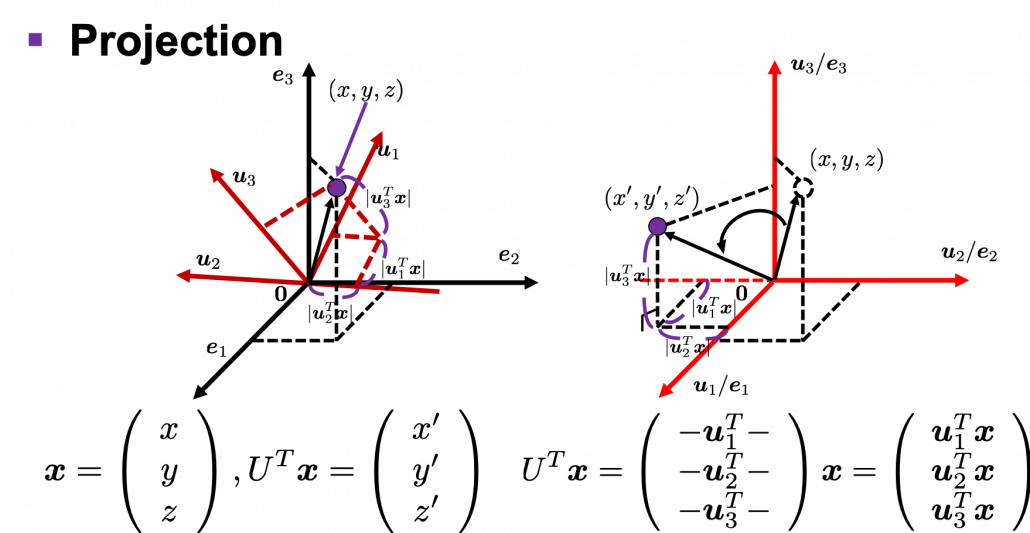
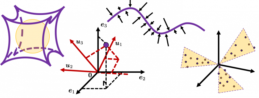
, with one corner of the cube located at the origin point of those axes. The purple dot denotes the corner of the cube directly opposite the origin corner. The cube is rotated in three dimensions, with the origin corner staying fixed in place. After the rotation with a pivot at the origin, the edges of the cube are now aligned with a new set of orthogonal axes (\boldsymbol{u}_1,  \boldsymbol{u}_2 , \boldsymbol{u}_3), shown in red. You might understand that more clearly with an equation: U\boldsymbol{x} = (\boldsymbol{u}_1 \: \boldsymbol{u}_2 \: \boldsymbol{u}_3) \left( \begin{array}{c} x \\ y \\ z \end{array} \right) = x\boldsymbol{u}_1 + y\boldsymbol{u}_2 + z\boldsymbol{u}_3. In short this rotation means you keep relative position of \boldsymbol{x}, I mean its coordinates (x, y, z), in the new orthonormal basis. In this article, let me call this a “cube rotation.”

The discussion above can be generalized to spaces with dimensions higher than 3. When U \in \mathbb{R}^{D \times D} 
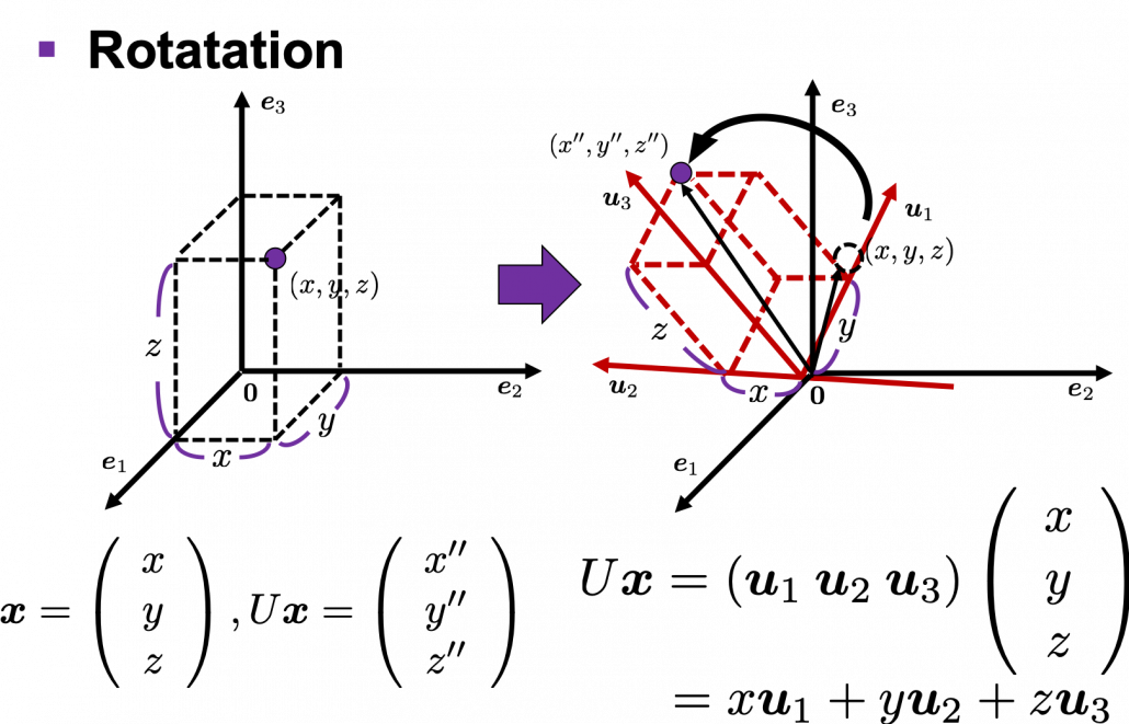
is an orthonormal matrix and a vector \boldsymbol{x} \in \mathbb{R}^D, you can project \boldsymbol{x} to \boldsymbol{x}' = U^T \boldsymbol{x}or rotate it to \boldsymbol{x}'' = U \boldsymbol{x}, where \boldsymbol{x}' = (x_{1}', \dots, x_{D}')^T and \boldsymbol{x}'' = (x_{1}'', \dots, x_{D}'')^T. In other words \boldsymbol{x} = U \boldsymbol{x}', which means you can rotate back \boldsymbol{x}' to the original point \boldsymbol{x} with the rotation matrix U.

I think you at least saw that rotation and projection are basically the same, and that is only a matter of how you look at the coordinate systems. But I would say the idea of projection is more important through out this article.

Let’s consider a function f(\boldsymbol{x}; A) = \boldsymbol{x}^T A \boldsymbol{x} = (\boldsymbol{x}, A \boldsymbol{x}), where A\in \mathbb{R}^{D\times D} is a real symmetric matrix. The distribution of f(\boldsymbol{x}; A) is quadratic curves whose center point covers the origin, and it is known that you can express this distribution in a much simpler way using eigenvectors. When you project this function on eigenvectors of A, that is when you substitute U \boldsymbol{x}' for \boldsymbol{x}, you get f = (\boldsymbol{x}, A \boldsymbol{x}) =(U \boldsymbol{x}', AU \boldsymbol{x}') = (\boldsymbol{x}')^T U^TAU \boldsymbol{x}' = (\boldsymbol{x}')^T \Lambda \boldsymbol{x}' = \lambda_1 ({x'}_1)^2 + \cdots + \lambda_D ({x'}_D)^2. You can always diagonalize real symmetric matrices, so the formula implies that the shapes of quadratic curves largely depend on eigenvectors. We are going to see this in detail in the next section.

*(\boldsymbol{x}, \boldsymbol{y}) denotes an inner product of \boldsymbol{x} and \boldsymbol{y}.

*We are going to see details of the shapes of quadratic “curves” or “functions” in the next section.

To be exact, you cannot naively multiply U or U^T for rotation. Let’s take a part of data I showed in the last article as an example. In the figure below, I projected data on the basis (\boldsymbol{u}_1,  \boldsymbol{u}_2 , \boldsymbol{u}_3).

You might have noticed that you cannot do a “cube rotation” in this case. If you make the coordinate system (\boldsymbol{u}_1, \boldsymbol{u}_2, \boldsymbol{u}_3) with your left hand, like you might have done in science classes in school to learn Fleming’s rule, you would soon realize that the coordinate systems in the figure above do not match. You need to flip the direction of one axis to match them.

Mathematically, you have to consider the determinant of the rotation matrix U. You can do a “cube rotation” when det(U)=1
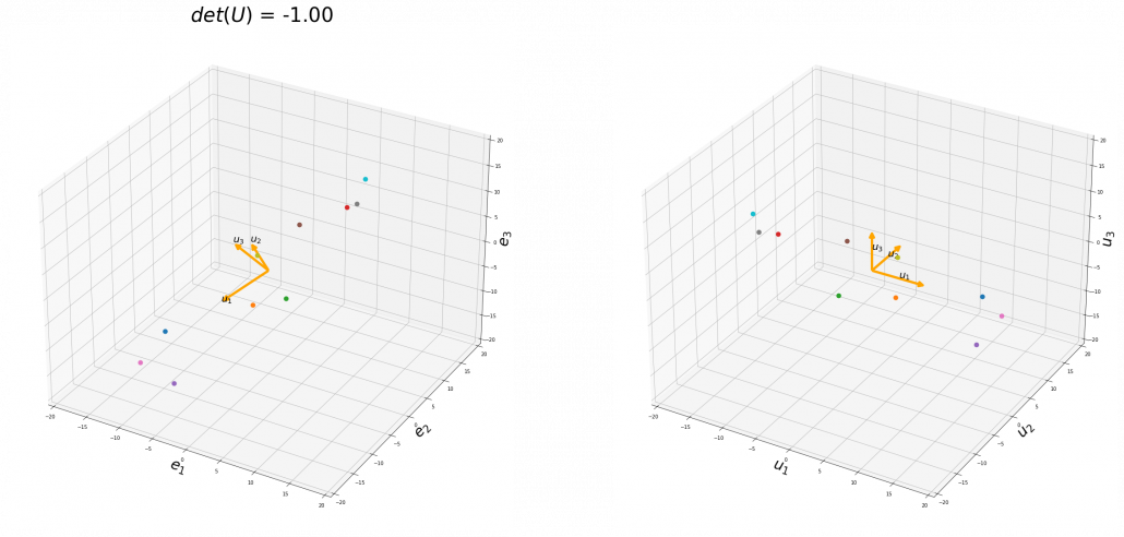
, and in the case above det(U) was -1, and you needed to flip one axis to make the determinant 1. In the example in the figure below, you can match the basis. This also can be generalized to higher dimensions, but that is also beyond the scope of this article series. If you are really interested, you should prepare some coffee and snacks and textbooks on linear algebra, and some weekends.

When you want to make general ellipsoids in a 3d space on Matplotlib, you can take advantage of rotation matrices. You first make a simple ellipsoid symmetric about xyz axis using polar coordinates, and you can rotate the whole ellipsoid with rotation matrices. I made some simple modules for drawing ellipsoid. If you put in a rotation matrix which diagonalize the covariance matrix of data and a list of three radiuses \sqrt{\lambda_1}, \sqrt{\lambda_2}, \sqrt{\lambda_3}
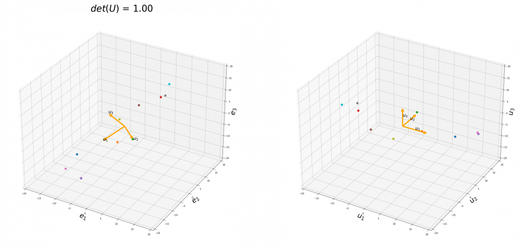
, you can rotate the original ellipsoid so that it fits the data well.
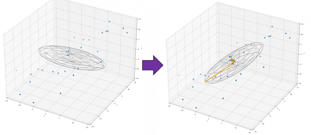
3 Types of quadratic curves.

*This article might look like a mathematical writing, but I would say this is more about computer science. Please tolerate some inaccuracy in terms of mathematics. I gave priority to visualizing necessary mathematical ideas in my article series. If you are not sure about details, please let me know.

In linear dimension reduction, or at least in this article series you mainly have to consider ellipsoids. However ellipsoids are just one type of quadratic curves. In the last article, I mentioned that when the center of a D dimensional ellipsoid is the origin point of a normal coordinate system, the formula of the surface of the ellipsoid is as follows: (\boldsymbol{x}, A\boldsymbol{x})=1, where A satisfies certain conditions. To be concrete, when (\boldsymbol{x}, A\boldsymbol{x})=1 is the surface of a ellipsoid, A has to be diagonalizable and positive definite.

*Real symmetric matrices are diagonalizable, and positive definite matrices have only positive eigenvalues. Covariance matrices \Sigma, whose displacement vectors I visualized in the last two articles, are known to be symmetric real matrices and positive semi-defintie. However, the surface of an ellipsoid which fit the data is \boldsymbol{x}^T \Sigma ^{-1} \boldsymbol{x} = const., not \boldsymbol{x}^T \Sigma \boldsymbol{x} = const..

*You have to keep it in mind that \boldsymbol{x} are all deviations.

*You do not have to think too much about what the “semi” of the term “positive semi-definite” means fow now.

As you could imagine, this is just one simple case of richer variety of graphs. Let’s consider a 3-dimensional space. Any quadratic curves in this space can be denoted as ax^2 + by^2 + cz^2 + dxy + eyz + fxz + px + qy + rz + s = 0, where at least one of a, b, c, d, e, f, p, q, r, s is not 0.  Let \boldsymbol{x} be (x, y, z)^T, then the quadratic curves can be simply denoted with a 3\times 3 matrix A and a 3-dimensional vector \boldsymbol{b} as follows: \boldsymbol{x}^T A\boldsymbol{x} + 2\boldsymbol{b}^T\boldsymbol{x} + s = 0, where A = \left( \begin{array}{ccc} a & \frac{d}{2} & \frac{f}{2} \\ \frac{d}{2} & b & \frac{e}{2} \\ \frac{f}{2} & \frac{e}{2} & c \end{array} \right), \boldsymbol{b} = \left( \begin{array}{c} \frac{p}{2} \\ \frac{q}{2} \\ \frac{r}{2} \end{array} \right). General quadratic curves are roughly classified into the 9 types below.
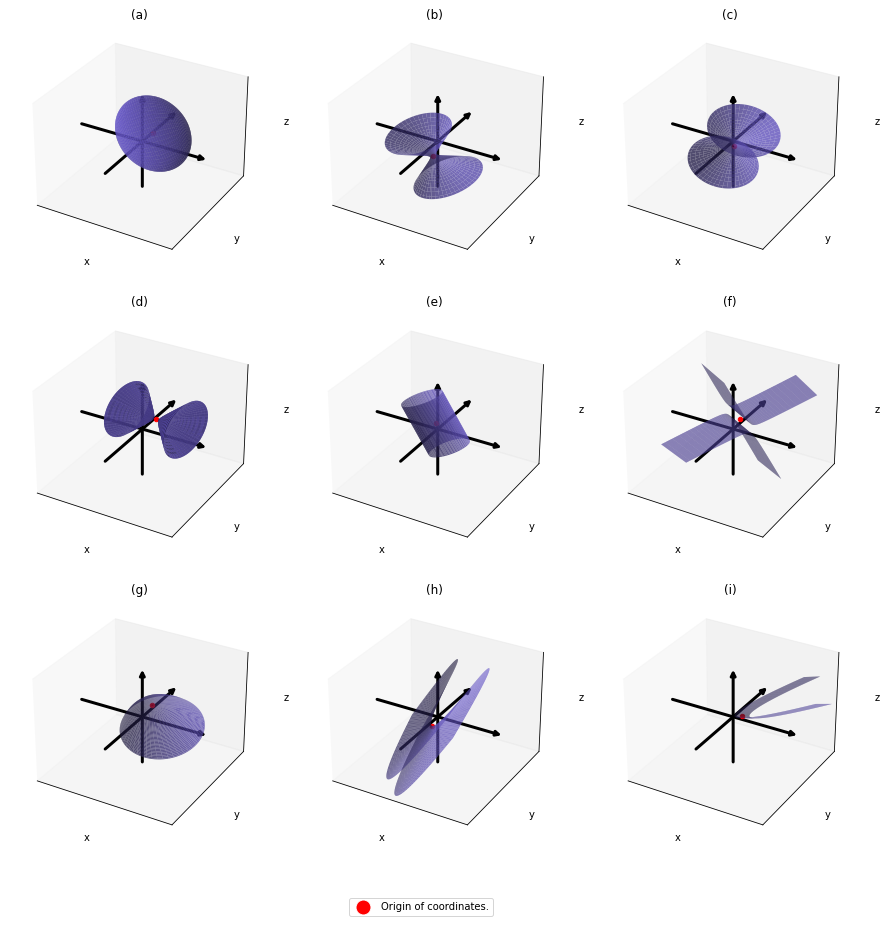
You can shift these quadratic curves so that their center points come to the origin, without rotation, and the resulting curves are as follows. The curves can be all denoted as \boldsymbol{x}^T A\boldsymbol{x}.

As you can see, A is a real symmetric matrix. As I have mentioned repeatedly, when all the elements of a D \times D symmetric matrix A are real values and its eigen values are \lambda_{i} (i=1, \dots , D), there exist orthogonal/orthonormal matrices U such that U^{-1}AU = \Lambda, where \Lambda = diag(\lambda_{1}, \dots , \lambda_{D}). Hence, you can diagonalize the A = \left( \begin{array}{ccc} a & \frac{d}{2} & \frac{f}{2} \\ \frac{d}{2} & b & \frac{e}{2} \\ \frac{f}{2} & \frac{e}{2} & c \end{array} \right) with an orthogonal matrix U. Let U be an orthogonal matrix such that U^T A U = \left( \begin{array}{ccc} \alpha  & 0 & 0 \\ 0 & \beta & 0 \\ 0 & 0 & \gamma \end{array} \right) =\left( \begin{array}{ccc} \lambda_1  & 0 & 0 \\ 0 & \lambda_2 & 0 \\ 0 & 0 & \lambda_3 \end{array} \right)
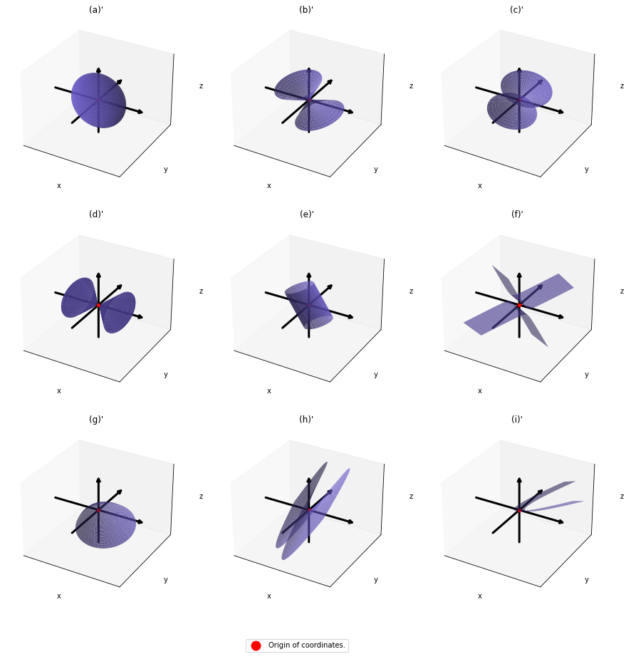
. After you apply rotation by
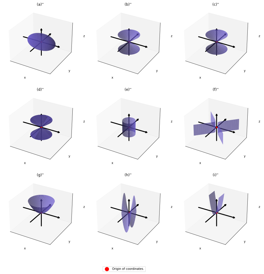
 U to the curves (a)” ~ (i)”, those curves are symmetrically placed about the xyz axes, and their center points still cross the origin. The resulting curves look like below. Or rather I should say you projected (a)’ ~ (i)’ on their eigenvectors.

In this article mainly (a)” , (g)”, (h)”, and (i)” are important. General equations for the curves is as follows

  • (a)”: \frac{x^2}{l^2} + \frac{y^2}{m^2} + \frac{z^2}{n^2} = 1
  • (g)”: z = \frac{x^2}{l^2} + \frac{y^2}{m^2}
  • (h)”: z = \frac{x^2}{l^2} - \frac{y^2}{m^2}
  • (i)”: z = \frac{x^2}{l^2}

, where l, m, n \in \mathbb{R}^+.

Even if this section has been puzzling to you, you just have to keep one point in your mind: we have been discussing general quadratic curves, but in PCA, you only need to consider a case where A is a covariance matrix, that is A=\Sigma. PCA corresponds to the case where you shift and rotate the curve (a) into (a)”. Subtracting the mean of data from each point of data corresponds to shifting quadratic curve (a) to (a)’. Calculating eigenvectors of A corresponds to calculating a rotation matrix U such that the curve (a)’ comes to (a)” after applying the rotation, or projecting curves on eigenvectors of \Sigma. Importantly we are only discussing the covariance of certain data, not the distribution of the data itself.

*Just in case you are interested in a little more mathematical sides: it is known that if you rotate all the points \boldsymbol{x} on the curve \boldsymbol{x}^T A\boldsymbol{x} + 2\boldsymbol{b}^T\boldsymbol{x} + s = 0 with the rotation matrix P, those points \boldsymbol{x} are mapped into a new quadratic curve \alpha x^2 + \beta y^2 + \gamma z^2 + \lambda x + \mu y + \nu z + \rho = 0. That means the rotation of the original quadratic curve with P (or rather rotating axes) enables getting rid of the terms xy, yz, zx. Also it is known that when \alpha ' \neq 0, with proper translations and rotations, the quadratic curve \alpha x^2 + \beta y^2 + \gamma z^2 + \lambda x + \mu y + \nu z + \rho = 0 can be mapped into one of the types of quadratic curves in the figure below, depending on coefficients of the original quadratic curve. And the discussion so far can be generalized to higher dimensional spaces, but that is beyond the scope of this article series. Please consult decent textbooks on linear algebra around you for further details.

4 Eigenvectors are gradients and sometimes variances.

In the second section I explained that you can express quadratic functions f(\boldsymbol{x}; A) = \boldsymbol{x}^T A \boldsymbol{x} in a very simple way by projecting \boldsymbol{x} on eigenvectors of A.

You can comprehend what I have explained in another way: eigenvectors, to be exact eigenvectors of real symmetric matrices A, are gradients. And in case of PCA, I mean when A=\Sigma eigenvalues are also variances. Before explaining what that means, let me explain a little of the totally common facts on mathematics. If you have variables \boldsymbol{x}\in \mathbb{R}^D, I think you can comprehend functions f(\boldysmbol{x}) in two ways. One is a normal “functions” f(\boldsymbol{x}), and the others are “curves” f(\boldsymbol{x}) = const.. “Functions” get an input \boldsymbol{x} and gives out an output f(\boldsymbol{x}), just as well as normal functions you would imagine. “Curves” are rather sets of \boldsymbol{x} \in \mathbb{R}^D such that f(\boldsymbol{x}) = const..

*Please assume that the terms “functions” and “curves” are my original words. I use them just in case I fail to use functions and curves properly.

The quadratic curves in the figure above are all “curves” in my term, which can be denoted as f(\boldsymbol{x}; A_3, \boldsymbol{b}_3)=const or f(\boldsymbol{x}; A_3)=const. However if you replace z of (g)”, (h)”, and (i)” with f, you can interpret the “curves” as “functions” which are denoted as f(\boldsymbol{x}; A_2). This might sounds too obvious to you, and my point is you can visualize how values of “functions” change only when the inputs are 2 dimensional.

When a symmetric 2\times 2 real matrices A_2 have two eigenvalues \lambda_1, \lambda_2
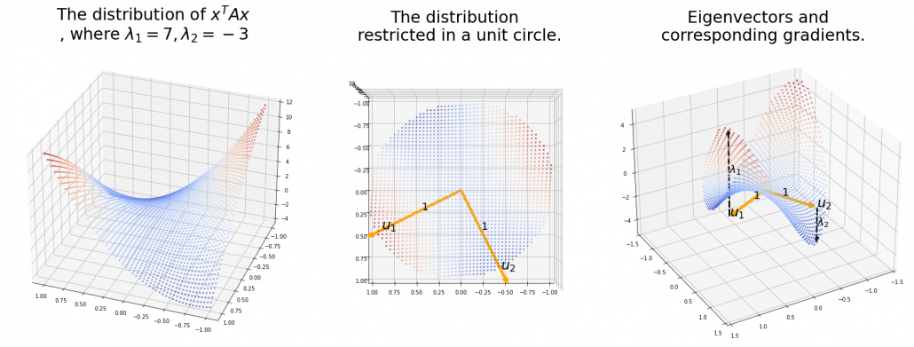
, the distribution of quadratic curves can be roughly classified to the following three types.

  • (g): Both \lambda_1 and \lambda_2 are positive or negative.
  • (h): Either of \lambda_1 or \lambda_2 is positive and the other is negative.
  • (i): Either of \lambda_1 or \lambda_2 is 0 and the other is not.

The equations of (g)” , (h)”, and (i)” correspond to each type of f=(\boldsymbol{x}; A_2), and thier curves look like the three graphs below.
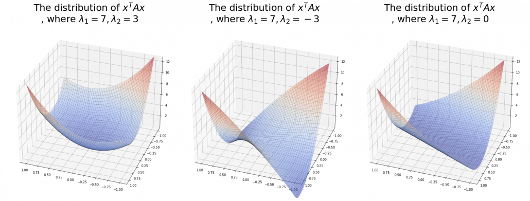
And in fact, when start from the origin and go in the direction of an eigenvector \boldsymbol{u}_i, \lambda_i is the gradient of the direction. You can see that more clearly when you restrict the distribution of f=(\boldsymbol{x}; A_2) to a unit circle. Like in the figure below, in case \lambda_1 = 7, \lambda_2 = 3, which is classified to (g), the distribution looks like the left side, and if you restrict the distribution in the unit circle, the distribution looks like a bowl like the middle and the right side. When you move in the direction of \boldsymbol{u}_1, you can climb the bowl as as high as \lambda_1, in \boldsymbol{u}_2 as high as \lambda_2.

Also in case of (h), the same facts hold. But in this case, you can also descend the curve.

*You might have seen the curve above in the context of optimization with stochastic gradient descent. The origin of the curve above is a notorious saddle point, where gradients are all 0 in any directions but not a local maximum or minimum. Points can be stuck in this point during optimization.

Especially in case of PCA, A is a covariance matrix, thus A=\Sigma. Eigenvalues of \Sigma are all equal to or greater than 0. And it is known that in this case \lambda_i is the variance of data projected on its corresponding eigenvector \boldsymbol{u}_i (i=0, \dots , D)
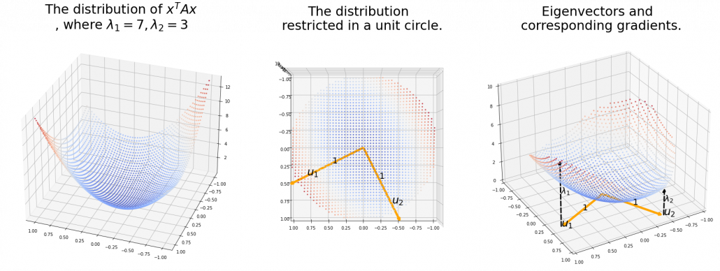
. Hence, if you project f(\boldsymbol{x}; \Sigma), quadratic curves formed by a covariance matrix \Sigma, on eigenvectors of \Sigma, you get f(\boldsymbol{x}; \Sigma) = ({x'}_1 \: \dots \: {x'}_D) (\lambda_1 {x'}_1 \: \dots \: \lambda_D {x'}_D)^t =\lambda_1 ({x'}_1)^2 + \cdots + \lambda_D ({x'}_D)^2.  This shows that you can re-weight ({x'}_1 \: \dots \: {x'}_D), the coordinates of data projected projected on eigenvectors of A, with \lambda_1, \dots, \lambda_D, which are variances ({x'}_1 \: \dots \: {x'}_D). As I mentioned in an example of data of exam scores in the last article, the bigger a variance \lambda_i is, the more the feature described by \boldsymbol{u}_i vary from sample to sample. In other words, you can ignore eigenvectors corresponding to small eigenvalues.

That is a great hint why principal components corresponding to large eigenvectors contain much information of the data distribution. And you can also interpret PCA as a “climbing” a bowl of f(\boldsymbol{x}; A_D), as I have visualized in the case of (g) type curve in the figure above.

*But as I have repeatedly mentioned, ellipsoid which fit data well isf(\boldsymbol{x}; \Sigma ^{-1}) =(\boldsymbol{x}')^T diag(\frac{1}{\lambda_1}, \dots, \frac{1}{\lambda_D})\boldsymbol{x}' = \frac{({x'}_{1})^2}{\lambda_1} + \cdots + \frac{({x'}_{D})^2}{\lambda_D} = const..

*You have to be careful that even if you slice a type (h) curve f(\boldsymbol{x}; A_D) with a place z=const
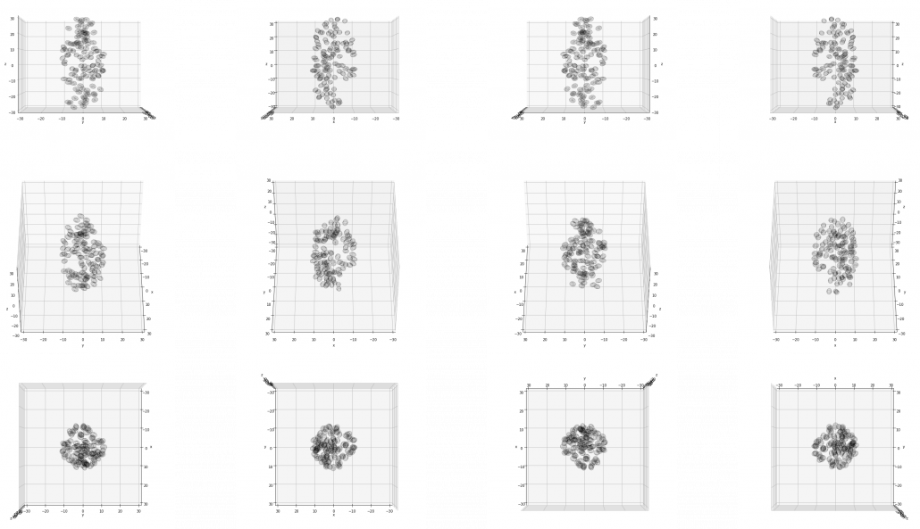
. the resulting cross section does not fit the original data well because the equation of the cross section is \lambda_1 ({x'}_1)^2 + \cdots + \lambda_D ({x'}_D)^2 = const. The figure below is an example of slicing the same f(\boldsymbol{x}; A_2) as the one above with z=1, and the resulting cross section.

As we have seen, \lambda_i, the eigenvalues of the covariance matrix of data are variances or data when projected on it eigenvectors. At the same time, when you fit an ellipsoid on the data, \sqrt{\lambda_i} 
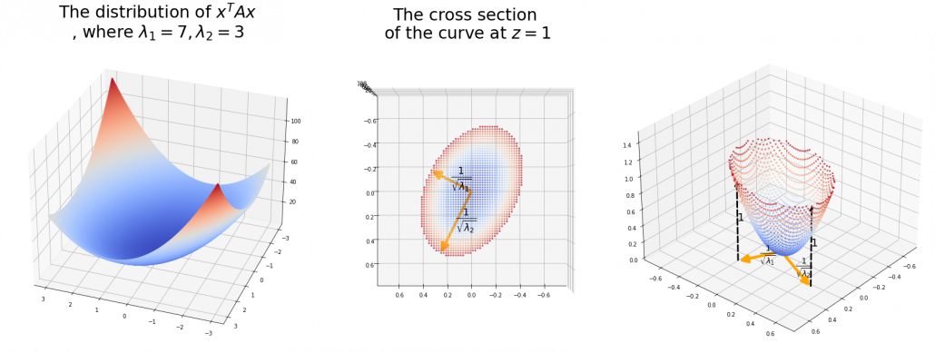
is the radius of the ellipsoid corresponding to \boldsymbol{u}_i. Thus ignoring data projected on eigenvectors corresponding to small eigenvalues is equivalent to cutting of the axes of the ellipsoid with small radiusses.

I have explained PCA in three different ways over three articles.

  • The second article: I focused on what kind of linear transformations convariance matrices \Sigma enable, by visualizing displacement vectors. And those vectors look like swirling and extending into directions of eigenvectors of \Sigma.
  • The third article: We directly found directions where certain data distribution “swell” the most, to find that data swell the most in directions of eigenvectors.
  • In this article, we have seen PCA corresponds to only one case of quadratic functions, where the matrix A is a covariance matrix. When you go in the directions of eigenvectors corresponding to big eigenvalues, the quadratic function increases the most. Also that means data samples have bigger variances when projected on the eigenvectors. Thus you can cut off eigenvectors corresponding to small eigenvectors because they retain little information about data, and that is equivalent to fitting an ellipsoid on data and cutting off axes with small radiuses.

*Let A be a covariance matrix, and you can diagonalize it with an orthogonal matrix U as follow: U^{T}AU = \Lambda, where \Lambda = diag(\lambda_1, \dots, \lambda_D). Thus A = U \Lambda U^{T}. U is a rotation, and multiplying a \boldsymbol{x} with \Lambda means you multiply each eigenvalue to each element of \boldsymbol{x}. At the end U^T enables the reverse rotation.

If you get data like the left side of the figure below, most explanation on PCA would just fit an oval on this data distribution. However after reading this articles series so far, you would have learned to see PCA from different viewpoints like at the right side of the figure below.


5 Ellipsoids in Gaussian distributions.

I have explained that if the covariance of a data distribution is \boldsymbol{\Sigma}
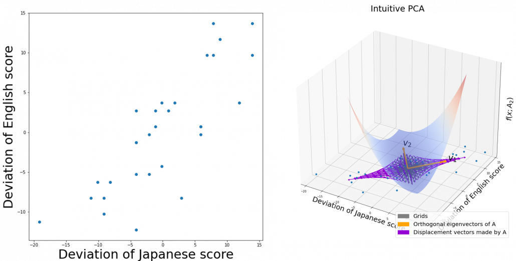
, the ellipsoid which fits the distribution the best is \bigl((\boldsymbol{x} - \boldsymbol{\mu}), \boldsymbol{\Sigma}^{-1}(\boldsymbol{x} - \boldsymbol{\mu})\bigr) = 1. You might have seen the part \bigl((\boldsymbol{x} - \boldsymbol{\mu}), \boldsymbol{\Sigma}^{-1}(\boldsymbol{x} - \boldsymbol{\mu})\bigr) = (\boldsymbol{x} - \boldsymbol{\mu}) \boldsymbol{\Sigma}^{-1}(\boldsymbol{x} - \boldsymbol{\mu}) somewhere else. It is the exponent of general Gaussian distributions: \mathcal{N}(\boldsymbol{x} | \boldsymbol{\mu}, \boldsymbol{\Sigma}) = \frac{1}{(2\pi)^{D/2}} \frac{1}{|\boldsymbol{\Sigma}|} exp\{ -\frac{1}{2}(\boldsymbol{x} - \boldsymbol{\mu}) \boldsymbol{\Sigma}^{-1}(\boldsymbol{x} - \boldsymbol{\mu}) \}.  It is known that the eigenvalues of \Sigma ^{-1} are \frac{1}{\lambda_1}, \dots, \frac{1}{\lambda_D}, and eigenvectors corresponding to each eigenvalue are also \boldsymbol{u}_1, \dots, \boldsymbol{u}_D respectively. Hence just as well as what we have seen, if you project (\boldsymbol{x} - \boldsymbol{\mu}) on each eigenvector of \Sigma ^{-1}, we can convert the exponent of the Gaussian distribution.

Let -\frac{1}{2}(\boldsymbol{x} - \boldsymbol{\mu}) \boldsymbol{\Sigma}^{-1}(\boldsymbol{x} - \boldsymbol{\mu}) be \boldsymbol{y} and U ^{-1} \boldsymbol{y}= U^{T} \boldsymbol{y} be \boldsymbol{y}', where U=(\boldsymbol{u}_1 \: \dots \: \boldsymbol{u}_D). Just as we have seen, (\boldsymbol{x} - \boldsymbol{\mu}) \boldsymbol{\Sigma}^{-1}(\boldsymbol{x} - \boldsymbol{\mu}) =\boldsymbol{y}^T\Sigma^{-1} \boldsymbol{y} =(U\boldsymbol{y}')^T \Sigma^{-1} U\boldsymbol{y}' =((\boldsymbol{y}')^T U^T \Sigma^{-1} U\boldsymbol{y}' = (\boldsymbol{y}')^T diag(\frac{1}{\lambda_1}, \dots, \frac{1}{\lambda_D}) \boldsymbol{y}' = \frac{({y'}_{1})^2}{\lambda_1} + \cdots + \frac{({y'}_{D})^2}{\lambda_D}. Hence \mathcal{N}(\boldsymbol{x} | \boldsymbol{\mu}, \boldsymbol{\Sigma}) = \frac{1}{(2\pi)^{D/2}} \frac{1}{|\boldsymbol{\Sigma}|} exp\{ -\frac{1}{2}(\boldsymbol{y}) \boldsymbol{\Sigma}^{-1}(\boldsymbol{y}) \} =  \frac{1}{(2\pi)^{D/2}} \frac{1}{|\boldsymbol{\Sigma}|} exp\{ -\frac{1}{2}(\frac{({y'}_{1})^2}{\lambda_1} + \cdots + \frac{({y'}_{D})^2}{\lambda_D} ) \} =\frac{1}{(2\pi)^{1/2}} \frac{1}{|\boldsymbol{\Sigma}|} exp\biggl( -\frac{1}{2} \frac{({y'}_{1})^2}{\lambda_1} \biggl) \cdots \frac{1}{(2\pi)^{1/2}} \frac{1}{|\boldsymbol{\Sigma}|} exp\biggl( -\frac{1}{2}\frac{({y'}_{D})^2}{\lambda_D} \biggl).

*To be mathematically exact about changing variants of normal distributions, you have to consider for example Jacobian matrices.

This results above demonstrate that, by projecting data on the eigenvectors of its covariance matrix, you can factorize the original multi-dimensional Gaussian distribution into a product of Gaussian distributions which are irrelevant to each other. However, at the same time, that is the potential limit of approximating data with PCA. This idea is going to be more important when you think about more probabilistic ways to handle PCA, which is more robust to lack of data.

I have explained PCA over 3 articles from various viewpoints. If you have been patient enough to read my article series, I think you have gained some deeper insight into not only PCA, but also linear algebra, and that should be helpful when you learn or teach data science. I hope my codes also help you. In fact these are not the only topics about PCA. There are a lot of important PCA-like algorithms.

In fact our expedition of ellipsoids, or PCA still continues, just as Star Wars series still continues. Especially if I have to explain an algorithm named probabilistic PCA, I need to explain the “Bayesian world” of machine learning. Most machine learning algorithms covered by major introductory textbooks tend to be too deterministic and dependent on the size of data. Many of those algorithms have another “parallel world,” where you can handle inaccuracy in better ways. I hope I can also write about them, and I might prepare another trilogy for such PCA. But I will not disappoint you, like “The Phantom Menace.”

Appendix: making a model of a bunch of grape with ellipsoid berries.

If you can control quadratic curves, reshaping and rotating them, you can make a model of a grape of olive bunch on Matplotlib. I made a program of making a model of a bunch of berries on Matplotlib using the module to draw ellipsoids which I introduced earlier. You can check the codes in this page.

*I have no idea how many people on this earth are in need of making such models.

I made some modules so that you can see the grape bunch from several angles. This might look very simple to you, but the locations of berries are organized carefully so that it looks like they are placed around a stem and that the berries are not too close to each other.


The programming code I created for this article is completly available here.

[Refereces]

[1]C. M. Bishop, “Pattern Recognition and Machine Learning,” (2006), Springer, pp. 78-83, 559-577

[2]「理工系新課程 線形代数 基礎から応用まで」, 培風館、(2017)

[3]「これなら分かる 最適化数学 基礎原理から計算手法まで」, 金谷健一著、共立出版, (2019), pp. 17-49

[4]「これなら分かる 応用数学教室 最小二乗法からウェーブレットまで」, 金谷健一著、共立出版, (2019), pp.165-208

[5] 「サボテンパイソン 」
https://sabopy.com/


How to make a toy English-German translator with multi-head attention heat maps: the overall architecture of Transformer

If you have been patient enough to read the former articles of this article series Instructions on Transformer for people outside NLP field, but with examples of NLP, you should have already learned a great deal of Transformer model, and I hope you gained a solid foundation of learning theoretical sides on this algorithm.

This article is going to focus more on practical implementation of a transformer model. We use codes in the Tensorflow official tutorial. They are maintained well by Google, and I think it is the best practice to use widely known codes.

The figure below shows what I have explained in the articles so far. Depending on your level of understanding, you can go back to my former articles. If you are familiar with NLP with deep learning, you can start with the third article.

1 The datasets

I think this article series appears to be on NLP, and I do believe that learning Transformer through NLP examples is very effective. But I cannot delve into effective techniques of processing corpus in each language. Thus we are going to use a library named BPEmb. This library enables you to encode any sentences in various languages into lists of integers. And conversely you can decode lists of integers to the language. Thanks to this library, we do not have to do simplification of alphabets, such as getting rid of Umlaut.

*Actually, I am studying in computer vision field, so my codes would look elementary to those in NLP fields.

The official Tensorflow tutorial makes a Portuguese-English translator, but in article we are going to make an English-German translator. Basically, only the codes below are my original. As I said, this is not an article on NLP, so all you have to know is that at every iteration you get a batch of (64, 41) sized tensor as the source sentences, and a batch of (64, 42) tensor as corresponding target sentences. 41, 42 are respectively the maximum lengths of the input or target sentences, and when input sentences are shorter than them, the rest positions are zero padded, as you can see in the codes below.

*If you just replace datasets and modules for encoding, you can make translators of other pairs of languages.

We are going to train a seq2seq-like Transformer model of converting those list of integers, thus a mapping from a vector to another vector. But each word, or integer is encoded as an embedding vector, so virtually the Transformer model is going to learn a mapping from sequence data to another sequence data. Let’s formulate this into a bit more mathematics-like way: when we get a pair of sequence data \boldsymbol{X} = (\boldsymbol{x}^{(1)}, \dots, \boldsymbol{x}^{(\tau _x)}) and \boldsymbol{Y} = (\boldsymbol{y}^{(1)}, \dots, \boldsymbol{y}^{(\tau _y)}), where \boldsymbol{x}^{(t)} \in \mathbb{R}^{|\mathcal{V}_{\mathcal{X}}|}, \boldsymbol{x}^{(t)} \in \mathbb{R}^{|\mathcal{V}_{\mathcal{Y}}|}
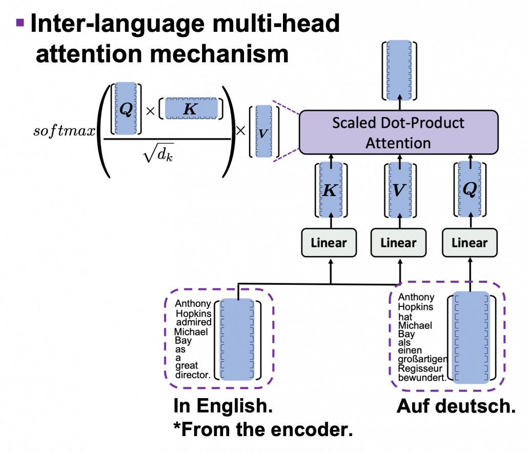
, respectively from English and German corpus, then we learn a mapping f: \boldsymbol{X} \to \boldsymbol{Y}.

*In this implementation the vocabulary sizes are both 10002. Thus |\mathcal{V}_{\mathcal{X}}|=|\mathcal{V}_{\mathcal{Y}}|=10002

2 The whole architecture

This article series has covered most of components of Transformer model, but you might not understand how seq2seq-like models can be constructed with them. It is very effective to understand how transformer is constructed by actually reading or writing codes, and in this article we are finally going to construct the whole architecture of a Transforme translator, following the Tensorflow official tutorial. At the end of this article, you would be able to make a toy English-German translator.

The implementation is mainly composed of 4 classes, EncoderLayer(), Encoder(), DecoderLayer(), and Decoder() class. The inclusion relations of the classes are displayed in the figure below.

To be more exact in a seq2seq-like model with Transformer, the encoder and the decoder are connected like in the figure below. The encoder part keeps converting input sentences in the original language through N 
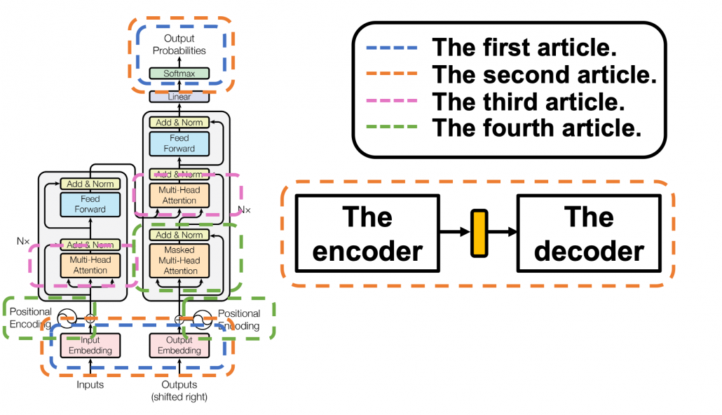
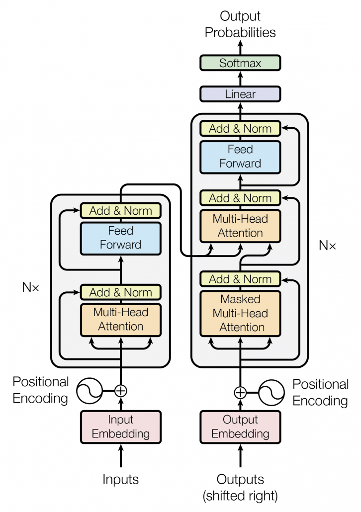
layers. The decoder part also keeps converting the inputs in the target languages, also through N layers, but it receives the output of the final layer of the Encoder at every layer.

You can see how the Encoder() class and the Decoder() class are combined in Transformer in the codes below. If you have used Tensorflow or Pytorch to some extent, the codes below should not be that hard to read.

3 The encoder

*From now on “sentences” do not mean only the input tokens in natural language, but also the reweighted and concatenated “values,” which I repeatedly explained in explained in the former articles. By the end of this section, you will see that Transformer repeatedly converts sentences layer by layer, remaining the shape of the original sentence.

I have explained multi-head attention mechanism in the third article, precisely, and I explained positional encoding and masked multi-head attention in the last article. Thus if you have read them and have ever written some codes in Tensorflow or Pytorch, I think the codes of Transformer in the official Tensorflow tutorial is not so hard to read. What is more, you do not use CNNs or RNNs in this implementation. Basically all you need is linear transformations. First of all let’s see how the EncoderLayer() and the Encoder() classes are implemented in the codes below.

You might be confused what “Feed Forward” means in  this article or the original paper on Transformer. The original paper says this layer is calculated as FFN(x) = max(0, xW_1 + b_1)W_2 +b_2. In short you stack two fully connected layers and activate it with a ReLU function. Let’s see how point_wise_feed_forward_network() function works in the implementation with some simple codes. As you can see from the number of parameters in each layer of the position wise feed forward neural network, the network does not depend on the length of the sentences.

From the number of parameters of the position-wise feed forward neural networks, you can see that you share the same parameters over all the positions of the sentences. That means in the figure above, you use the same densely connected layers at all the positions, in single layer. But you also have to keep it in mind that parameters for position-wise feed-forward networks change from layer to layer. That is also true of “Layer” parts in Transformer model, including the output part of the decoder: there are no learnable parameters which cover over different positions of tokens. These facts lead to one very important feature of Transformer: the number of parameters does not depend on the length of input or target sentences. You can offset the influences of the length of sentences with multi-head attention mechanisms. Also in the decoder part, you can keep the shape of sentences, or reweighted values, layer by layer, which is expected to enhance calculation efficiency of Transformer models.

4, The decoder

The structures of DecoderLayer() and the Decoder() classes are quite similar to those of EncoderLayer() and the Encoder() classes, so if you understand the last section, you would not find it hard to understand the codes below. What you have to care additionally in this section is inter-language multi-head attention mechanism. In the third article I was repeatedly explaining multi-head self attention mechanism, taking the input sentence “Anthony Hopkins admired Michael Bay as a great director.” as an example. However, as I explained in the second article, usually in attention mechanism, you compare sentences with the same meaning in two languages. Thus the decoder part of Transformer model has not only self-attention multi-head attention mechanism of the target sentence, but also an inter-language multi-head attention mechanism. That means, In case of translating from English to German, you compare the sentence “Anthony Hopkins hat Michael Bay als einen großartigen Regisseur bewundert.” with the sentence itself in masked multi-head attention mechanism (, just as I repeatedly explained in the third article). On the other hand, you compare “Anthony Hopkins hat Michael Bay als einen großartigen Regisseur bewundert.” with “Anthony Hopkins admired Michael Bay as a great director.” in the inter-language multi-head attention mechanism (, just as you can see in the figure above).

*The “inter-language multi-head attention mechanism” is my original way to call it.

I briefly mentioned how you calculate the inter-language multi-head attention mechanism in the end of the third article, with some simple codes, but let’s see that again, with more straightforward figures. If you understand my explanation on multi-head attention mechanism in the third article, the inter-language multi-head attention mechanism is nothing difficult to understand. In the multi-head attention mechanism in encoder layers, “queries”, “keys”, and “values” come from the same sentence in English, but in case of inter-language one, only “keys” and “values” come from the original sentence, and “queries” come from the target sentence. You compare “queries” in German with the “keys” in the original sentence in English, and you re-weight the sentence in English. You use the re-weighted English sentence in the decoder part, and you do not need look-ahead mask in this inter-language multi-head attention mechanism.

Just as well as multi-head self-attention, you can calculate inter-language multi-head attention mechanism as follows: softmax(\frac{\boldsymbol{Q} \boldsymbol{K} ^T}{\sqrt{d}_k})
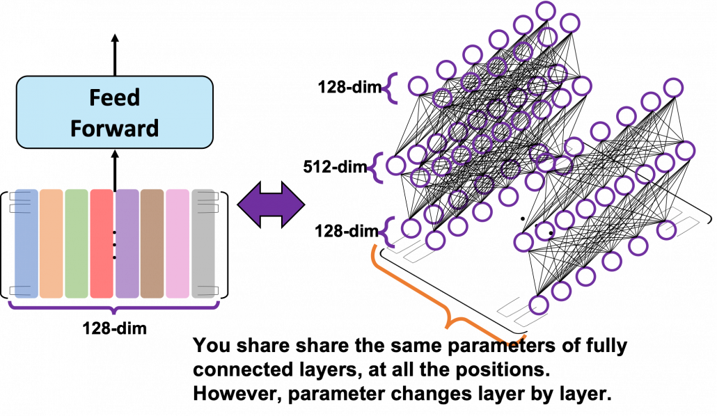
. In the example above, the resulting multi-head attention map is a 10 \times 9 matrix like in the figure below.

Once you keep the points above in you mind, the implementation of the decoder part should not be that hard.

5 Masking tokens in practice

I explained masked-multi-head attention mechanism in the last article, and the ideas itself is not so difficult. However in practice this is implemented in a little tricky way. You might have realized that the size of input matrices is fixed so that it fits the longest sentence. That means, when the maximum length of the input sentences is 41, even if the sentences in a batch have less than 41 tokens, you sample (64, 41) sized tensor as a batch every time (The 64 is a batch size). Let “Anthony Hopkins admired Michael Bay as a great director.”, which has 9 tokens in total, be an input. We have been considering calculating (9, 9) sized attention maps or (10, 9) sized attention maps, but in practice you use (41, 41) or (42, 41) sized ones. When it comes to calculating self attentions in the encoder part, you zero pad self attention maps with encoder padding masks, like in the figure below. The black dots denote the zero valued elements.

As you can see in the codes below, encode padding masks are quite simple. You just multiply the padding masks with -1e9 and add them to attention maps and apply a softmax function. Thereby you can zero-pad the columns in the positions/columns where you added -1e9 to.

I explained look ahead mask in the last article, and in practice you combine normal padding masks and look ahead masks like in the figure below. You can see that you can compare each token with only its previous tokens. For example you can compare “als” only with “Anthony”, “Hopkins”, “hat”, “Michael”, “Bay”, “als”, not with “einen”, “großartigen”, “Regisseur” or “bewundert.”

Decoder padding masks are almost the same as encoder one. You have to keep it in mind that you zero pad positions which surpassed the length of the source input sentence.

6 Decoding process

In the last section we have seen that we can zero-pad columns, but still the rows are redundant. However I guess that is not a big problem because you decode the final output in the direction of the rows of attention maps. Once you decode <end> token, you stop decoding. The redundant rows would not affect the decoding anymore.

This decoding process is similar to that of seq2seq models with RNNs, and that is why you need to hide future tokens in the self-multi-head attention mechanism in the decoder. You share the same densely connected layers followed by a softmax function, at all the time steps of decoding. Transformer has to learn how to decode only based on the words which have appeared so far.

According to the original paper, “We also modify the self-attention sub-layer in the decoder stack to prevent positions from attending to subsequent positions. This masking, combined with fact that the output embeddings are offset by one position, ensures that the predictions for position i 
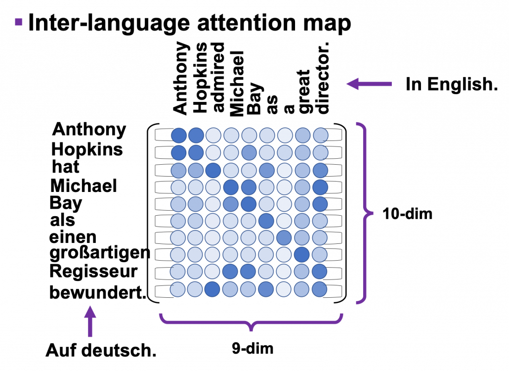
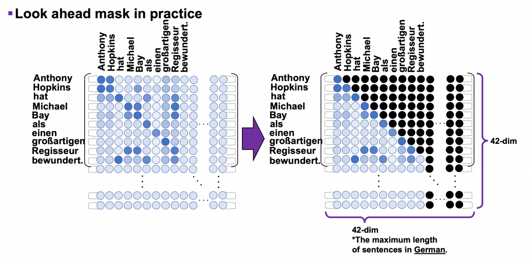
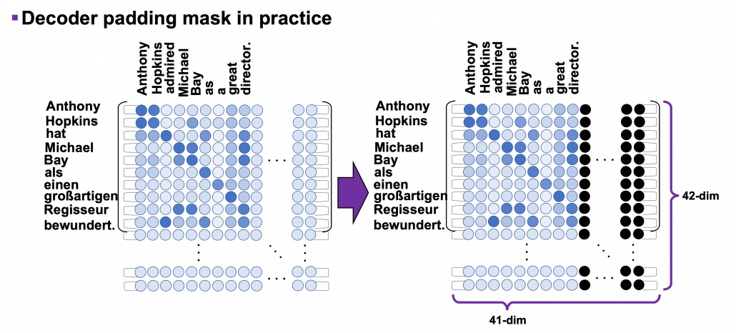
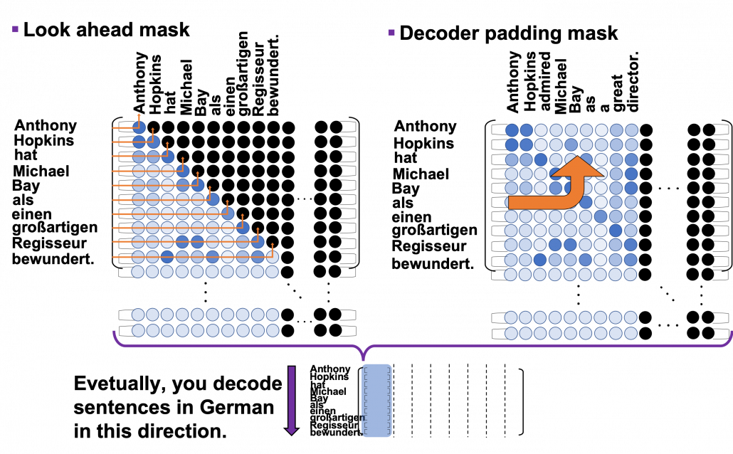
can depend only on the known outputs at positions less than i.” After these explanations, I think you understand the part more clearly.

The codes blow is for the decoding part. You can see that you first start decoding an output sentence with a sentence composed of only <start>, and you decide which word to decoded, step by step.

*It easy to imagine that this decoding procedure is not the best. In reality you have to consider some possibilities of decoding, and you can do that with beam search decoding.

After training this English-German translator for 30 epochs you can translate relatively simple English sentences into German. I displayed some results below, with heat maps of multi-head attention. Each colored attention maps corresponds to each head of multi-head attention. The examples below are all from the fourth (last) layer, but you can visualize maps in any layers. When it comes to look ahead attention, naturally only the lower triangular part of the maps is activated.

This article series has not covered some important topics machine translation, for example how to calculate translation errors. Actually there are many other fascinating topics related to machine translation. For example beam search decoding, which consider some decoding possibilities, or other topics like how to handle proper nouns such as “Anthony” or “Hopkins.” But this article series is not on NLP. I hope you could effectively learn the architecture of Transformer model with examples of languages so far. And also I have not explained some details of training the network, but I will not cover that because I think that depends on tasks. The next article is going to be the last one of this series, and I hope you can see how Transformer is applied in computer vision fields, in a more “linguistic” manner.

But anyway we have finally made it. In this article series we have seen that one of the earliest computers was invented to break Enigma. And today we can quickly make a more or less accurate translator on our desk. With Transformer models, you can even translate deadly funny jokes into German.

*You can train a translator with this code.

*After training a translator, you can translate English sentences into German with this code.

[References]

[1] Ashish Vaswani, Noam Shazeer, Niki Parmar, Jakob Uszkoreit, Llion Jones, Aidan N. Gomez, Lukasz Kaiser, Illia Polosukhin, “Attention Is All You Need” (2017)

[2] “Transformer model for language understanding,” Tensorflow Core
https://www.tensorflow.org/overview

[3] Jay Alammar, “The Illustrated Transformer,”
http://jalammar.github.io/illustrated-transformer/

[4] “Stanford CS224N: NLP with Deep Learning | Winter 2019 | Lecture 14 – Transformers and Self-Attention,” stanfordonline, (2019)
https://www.youtube.com/watch?v=5vcj8kSwBCY

[5]Tsuboi Yuuta, Unno Yuuya, Suzuki Jun, “Machine Learning Professional Series: Natural Language Processing with Deep Learning,” (2017), pp. 91-94
坪井祐太、海野裕也、鈴木潤 著, 「機械学習プロフェッショナルシリーズ 深層学習による自然言語処理」, (2017), pp. 191-193

* I make study materials on machine learning, sponsored by DATANOMIQ. I do my best to make my content as straightforward but as precise as possible. I include all of my reference sources. If you notice any mistakes in my materials, including grammatical errors, please let me know (email: yasuto.tamura@datanomiq.de). And if you have any advice for making my materials more understandable to learners, I would appreciate hearing it.

Multi-head attention mechanism: “queries”, “keys”, and “values,” over and over again

This is the third article of my article series named “Instructions on Transformer for people outside NLP field, but with examples of NLP.”

In the last article, I explained how attention mechanism works in simple seq2seq models with RNNs, and it basically calculates correspondences of the hidden state at every time step, with all the outputs of the encoder. However I would say the attention mechanisms of RNN seq2seq models use only one standard for comparing them. Using only one standard is not enough for understanding languages, especially when you learn a foreign language. You would sometimes find it difficult to explain how to translate a word in your language to another language. Even if a pair of languages are very similar to each other, translating them cannot be simple switching of vocabulary. Usually a single token in one language is related to several tokens in the other language, and vice versa. How they correspond to each other depends on several criteria, for example “what”, “who”, “when”, “where”, “why”, and “how”. It is easy to imagine that you should compare tokens with several criteria.

Transformer model was first introduced in the original paper named “Attention Is All You Need,” and from the title you can easily see that attention mechanism plays important roles in this model. When you learn about Transformer model, you will see the figure below, which is used in the original paper on Transformer.  This is the simplified overall structure of one layer of Transformer model, and you stack this layer N times. In one layer of Transformer, there are three multi-head attention, which are displayed as boxes in orange. These are the very parts which compare the tokens on several standards. I made the head article of this article series inspired by this multi-head attention mechanism.

The figure below is also from the original paper on Transfromer. If you can understand how multi-head attention mechanism works with the explanations in the paper, and if you have no troubles understanding the codes in the official Tensorflow tutorial, I have to say this article is not for you. However I bet that is not true of majority of people, and at least I need one article to clearly explain how multi-head attention works. Please keep it in mind that this article covers only the architectures of the two figures below. However multi-head attention mechanisms are crucial components of Transformer model, and throughout this article, you would not only see how they work but also get a little control over it at an implementation level.

1 Multi-head attention mechanism

When you learn Transformer model, I recommend you first to pay attention to multi-head attention. And when you learn multi-head attentions, before seeing what scaled dot-product attention is, you should understand the whole structure of multi-head attention, which is at the right side of the figure above. In order to calculate attentions with a “query”, as I said in the last article, “you compare the ‘query’ with the ‘keys’ and get scores/weights for the ‘values.’ Each score/weight is in short the relevance between the ‘query’ and each ‘key’. And you reweight the ‘values’ with the scores/weights, and take the summation of the reweighted ‘values’.” Sooner or later, you will notice I would be just repeating these phrases over and over again throughout this article, in several ways.

*Even if you are not sure what “reweighting” means in this context, please keep reading. I think you would little by little see what it means especially in the next section.

The overall process of calculating multi-head attention, displayed in the figure above, is as follows (Please just keep reading. Please do not think too much.): first you split the V: “values”, K: “keys”, and Q: “queries”, and second you transform those divided “values”, “keys”, and “queries” with densely connected layers (“Linear” in the figure). Next you calculate attention weights and reweight the “values” and take the summation of the reiweighted “values”, and you concatenate the resulting summations. At the end you pass the concatenated “values” through another densely connected layers. The mechanism of scaled dot-product attention is just a matter of how to concretely calculate those attentions and reweight the “values”.

*In the last article I briefly mentioned that “keys” and “queries” can be in the same language. They can even be the same sentence in the same language, and in this case the resulting attentions are called self-attentions, which we are mainly going to see. I think most people calculate “self-attentions” unconsciously when they speak. You constantly care about what “she”, “it” , “the”, or “that” refers to in you own sentence, and we can say self-attention is how these everyday processes is implemented.

Let’s see the whole process of calculating multi-head attention at a little abstract level. From now on, we consider an example of calculating multi-head self-attentions, where the input is a sentence “Anthony Hopkins admired Michael Bay as a great director.” In this example, the number of tokens is 9, and each token is encoded as a 512-dimensional embedding vector. And the number of heads is 8. In this case, as you can see in the figure below, the input sentence “Anthony Hopkins admired Michael Bay as a great director.” is implemented as a 9\times 512 
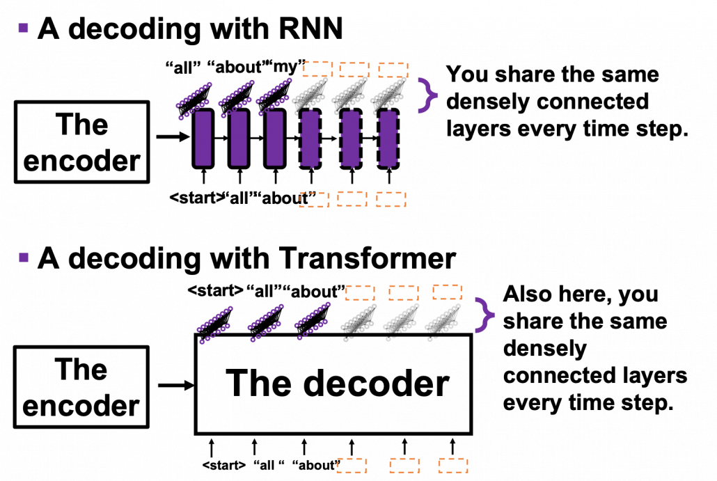
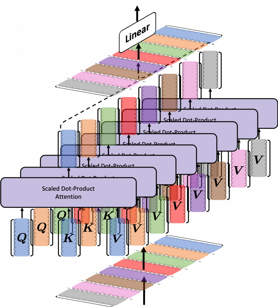
matrix. You first split each token into 512/8=64 dimensional, 8 vectors in total, as I colored in the figure below. In other words, the input matrix is divided into 8 colored chunks, which are all 9\times 64 matrices, but each colored matrix expresses the same sentence. And you calculate self-attentions of the input sentence independently in the 8 heads, and you reweight the “values” according to the attentions/weights. After this, you stack the sum of the reweighted “values”  in each colored head, and you concatenate the stacked tokens of each colored head. The size of each colored chunk does not change even after reweighting the tokens. According to Ashish Vaswani, who invented Transformer model, each head compare “queries” and “keys” on each standard. If the a Transformer model has 4 layers with 8-head multi-head attention , at least its encoder has 4\times 8 = 32 heads, so the encoder learn the relations of tokens of the input on 32 different standards.
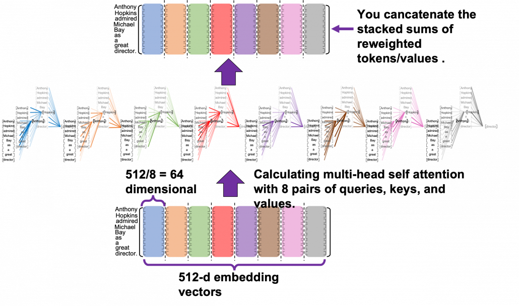
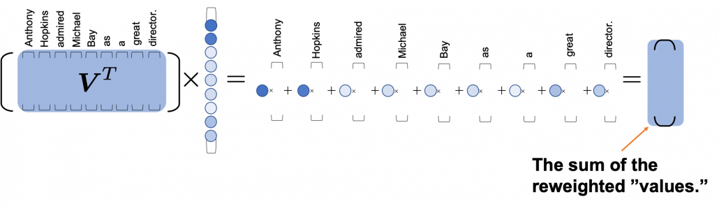
I think you now have rough insight into how you calculate multi-head attentions. In the next section I am going to explain the process of reweighting the tokens, that is, I am finally going to explain what those colorful lines in the head image of this article series are.

*Each head is randomly initialized, so they learn to compare tokens with different criteria. The standards might be straightforward like “what” or “who”, or maybe much more complicated. In attention mechanisms in deep learning, you do not need feature engineering for setting such standards.

2 Calculating attentions and reweighting “values”

If you have read the last article or if you understand attention mechanism to some extent, you should already know that attention mechanism calculates attentions, or relevance between “queries” and “keys.” In the last article, I showed the idea of weights as a histogram, and in that case the “query” was the hidden state of the decoder at every time step, whereas the “keys” were the outputs of the encoder. In this section, I am going to explain attention mechanism in a more abstract way, and we consider comparing more general “tokens”, rather than concrete outputs of certain networks. In this section each [ \cdots ] denotes a token, which is usually an embedding vector in practice.

Please remember this mantra of attention mechanism: “you compare the ‘query’ with the ‘keys’ and get scores/weights for the ‘values.’ Each score/weight is in short the relevance between the ‘query’ and each ‘key’. And you reweight the ‘values’ with the scores/weights, and take the summation of the reweighted ‘values’.” The figure below shows an overview of a case where “Michael” is a query. In this case you compare the query with the “keys”, that is, the input sentence “Anthony Hopkins admired Michael Bay as a great director.” and you get the histogram of attentions/weights. Importantly the sum of the weights 1. With the attentions you have just calculated, you can reweight the “values,” which also denote the same input sentence. After that you can finally take a summation of the reweighted values. And you use this summation.

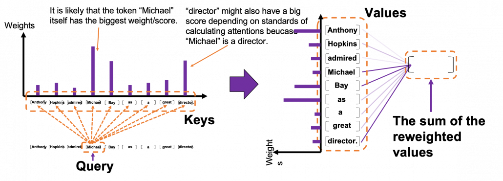
*I have been repeating the phrase “reweighting ‘values’  with attentions,”  but you in practice calculate the sum of those reweighted “values.”

Assume that compared to the “query”  token “Michael”, the weights of the “key” tokens “Anthony”, “Hopkins”, “admired”, “Michael”, “Bay”, “as”, “a”, “great”, and “director.” are respectively 0.06, 0.09, 0.05, 0.25, 0.18, 0.06, 0.09, 0.06, 0.15. In this case the sum of the reweighted token is 0.06″Anthony” + 0.09″Hopkins” + 0.05″admired” + 0.25″Michael” + 0.18″Bay” + 0.06″as” + 0.09″a” + 0.06″great” 0.15″director.”, and this sum is the what wee actually use.

*Of course the tokens are embedding vectors in practice. You calculate the reweighted vector in actual implementation.

You repeat this process for all the “queries.”  As you can see in the figure below, you get summations of 9 pairs of reweighted “values” because you use every token of the input sentence “Anthony Hopkins admired Michael Bay as a great director.” as a “query.” You stack the sum of reweighted “values” like the matrix in purple in the figure below, and this is the output of a one head multi-head attention.

3 Scaled-dot product

This section is a only a matter of linear algebra. Maybe this is not even so sophisticated as linear algebra. You just have to do lots of Excel-like operations. A tutorial on Transformer by Jay Alammar is also a very nice study material to understand this topic with simpler examples. I tried my best so that you can clearly understand multi-head attention at a more mathematical level, and all you need to know in order to read this section is how to calculate products of matrices or vectors, which you would see in the first some pages of textbooks on linear algebra.

We have seen that in order to calculate multi-head attentions, we prepare 8 pairs of “queries”, “keys” , and “values”, which I showed in 8 different colors in the figure in the first section. We calculate attentions and reweight “values” independently in 8 different heads, and in each head the reweighted “values” are calculated with this very simple formula of scaled dot-product: Attention(\boldsymbol{Q}, \boldsymbol{K}, \boldsymbol{V}) =softmax(\frac{\boldsymbol{Q} \boldsymbol{K} ^T}{\sqrt{d}_k})\boldsymbol{V}
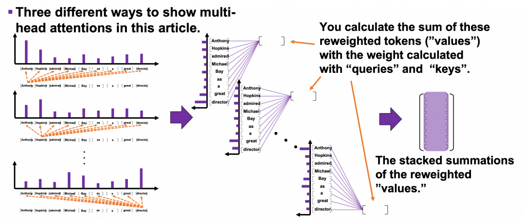
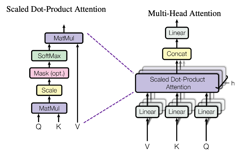
. Let’s take an example of calculating a scaled dot-product in the blue head.

At the left side of the figure below is a figure from the original paper on Transformer, which explains one-head of multi-head attention. If you have read through this article so far, the figure at the right side would be more straightforward to understand. You divide the input sentence into 8 chunks of matrices, and you independently put those chunks into eight head. In one head, you convert the input matrix by three different fully connected layers, which is “Linear” in the figure below, and prepare three matrices Q, K, V, which are “queries”, “keys”, and “values” respectively.

*Whichever color attention heads are in, the processes are all the same.

*You divide \frac{\boldsymbol{Q} \boldsymbol{K}} ^T by \sqrt{d}_k in the formula. According to the original paper, it is known that re-scaling
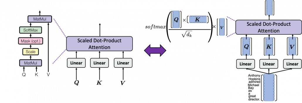
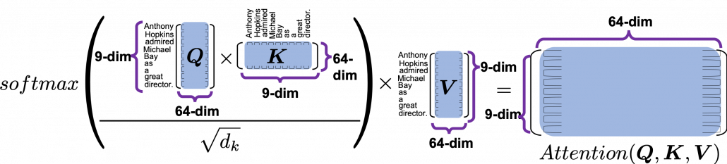
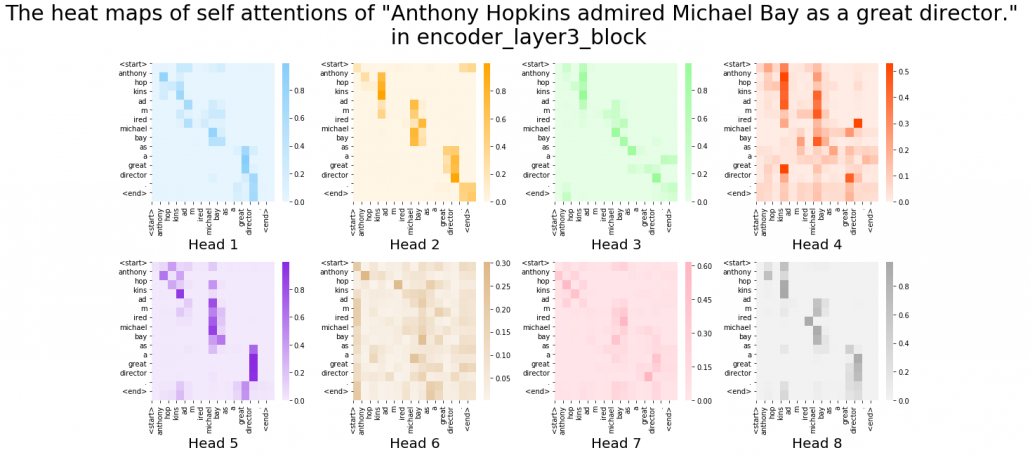
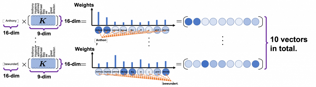
 \frac{\boldsymbol{Q} \boldsymbol{K}} ^T by \sqrt{d}_k is found to be effective. I am not going to discuss why in this article.

As you can see in the figure below, calculating Attention(\boldsymbol{Q}, \boldsymbol{K}, \boldsymbol{V}) is virtually just multiplying three matrices with the same size (Only K is transposed though). The resulting 9\times 64 matrix is the output of the head.

softmax(\frac{\boldsymbol{Q} \boldsymbol{K} ^T}{\sqrt{d}_k}) is calculated like in the figure below. The softmax function regularize each row of the re-scaled product \frac{\boldsymbol{Q} \boldsymbol{K} ^T}{\sqrt{d}_k}, and the resulting 9\times 9 matrix is a kind a heat map of self-attentions.

The process of comparing one “query” with “keys” is done with simple multiplication of a vector and a matrix, as you can see in the figure below. You can get a histogram of attentions for each query, and the resulting 9 dimensional vector is a list of attentions/weights, which is a list of blue circles in the figure below. That means, in Transformer model, you can compare a “query” and a “key” only by calculating an inner product. After re-scaling the vectors by dividing them with \sqrt{d_k} 
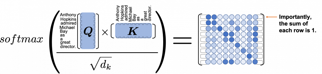
and regularizing them with a softmax function, you stack those vectors, and the stacked vectors is the heat map of attentions.

You can reweight “values” with the heat map of self-attentions, with simple multiplication. It would be more straightforward if you consider a transposed scaled dot-product \boldsymbol{V}^T \cdot softmax(\frac{\boldsymbol{Q} \boldsymbol{K} ^T}{\sqrt{d}_k})^T. This also should be easy to understand if you know basics of linear algebra.

One column of the resulting matrix (\boldsymbol{V}^T \cdot softmax(\frac{\boldsymbol{Q} \boldsymbol{K} ^T}{\sqrt{d}_k})^T) can be calculated with a simple multiplication of a matrix and a vector, as you can see in the figure below. This corresponds to the process or “taking a summation of reweighted ‘values’,” which I have been repeating. And I would like you to remember that you got those weights (blue) circles by comparing a “query” with “keys.”

Again and again, let’s repeat the mantra of attention mechanism together: “you compare the ‘query’ with the ‘keys’ and get scores/weights for the ‘values.’ Each score/weight is in short the relevance between the ‘query’ and each ‘key’. And you reweight the ‘values’ with the scores/weights, and take the summation of the reweighted ‘values’.” If you have been patient enough to follow my explanations, I bet you have got a clear view on how multi-head attention mechanism works.

We have been seeing the case of the blue head, but you can do exactly the same procedures in every head, at the same time, and this is what enables parallelization of multi-head attention mechanism. You concatenate the outputs of all the heads, and you put the concatenated matrix through a fully connected layers.

If you are reading this article from the beginning, I think this section is also showing the same idea which I have repeated, and I bet more or less you no have clearer views on how multi-head attention mechanism works. In the next section we are going to see how this is implemented.

4 Tensorflow implementation of multi-head attention

Let’s see how multi-head attention is implemented in the Tensorflow official tutorial. If you have read through this article so far, this should not be so difficult. I also added codes for displaying heat maps of self attentions. With the codes in this Github page, you can display self-attention heat maps for any input sentences in English.

The multi-head attention mechanism is implemented as below. If you understand Python codes and Tensorflow to some extent, I think this part is relatively easy.  The multi-head attention part is implemented as a class because you need to train weights of some fully connected layers. Whereas, scaled dot-product is just a function.

*I am going to explain the create_padding_mask() and create_look_ahead_mask() functions in upcoming articles. You do not need them this time.

Let’s see a case of using multi-head attention mechanism on a (1, 9, 512) sized input tensor, just as we have been considering in throughout this article. The first axis of (1, 9, 512) corresponds to the batch size, so this tensor is virtually a (9, 512) sized tensor, and this means the input is composed of 9 512-dimensional vectors. In the results below, you can see how the shape of input tensor changes after each procedure of calculating multi-head attention. Also you can see that the output of the multi-head attention is the same as the input, and you get a 9\times 9 matrix of attention heat maps of each attention head.

I guess the most complicated part of this implementation above is the split_head() function, especially if you do not understand tensor arithmetic. This part corresponds to splitting the input tensor to 8 different colored matrices as in one of the figures above. If you cannot understand what is going on in the function, I recommend you to prepare a sample tensor as below.

This is just a simple (1, 9, 512) sized tensor with sequential integer elements. The first row (1, 2, …., 512) corresponds to the first input token, and (4097, 4098, … , 4608) to the last one. You should try converting this sample tensor to see how multi-head attention is implemented. For example you can try the operations below.

These operations correspond to splitting the input into 8 heads, whose sizes are all (9, 64). And the second axis of the resulting (1, 8, 9, 64) tensor corresponds to the index of the heads. Thus sample_sentence[0][0] corresponds to the first head, the blue 9\times 64 matrix. Some Tensorflow functions enable linear calculations in each attention head, independently as in the codes below.

Very importantly, we have been only considering the cases of calculating self attentions, where all “queries”, “keys”, and “values” come from the same sentence in the same language. However, as I showed in the last article, usually “queries” are in a different language from “keys” and “values” in translation tasks, and “keys” and “values” are in the same language. And as you can imagine, usualy “queries” have different number of tokens from “keys” or “values.” You also need to understand this case, which is not calculating self-attentions. If you have followed this article so far, this case is not that hard to you. Let’s briefly see an example where the input sentence in the source language is composed 9 tokens, on the other hand the output is composed 12 tokens.

As I mentioned, one of the outputs of each multi-head attention class is 9\times 9 matrix of attention heat maps, which I displayed as a matrix composed of blue circles in the last section. The the implementation in the Tensorflow official tutorial, I have added codes to display actual heat maps of any input sentences in English.

*If you want to try displaying them by yourself, download or just copy and paste codes in this Github page. Please maker “datasets” directory in the same directory as the code. Please download “spa-eng.zip” from this page, and unzip it. After that please put “spa.txt” on the “datasets” directory. Also, please download the “checkpoints_en_es” folder from this link, and place the folder in the same directory as the file in the Github page. In the upcoming articles, you would need similar processes to run my codes.

After running codes in the Github page, you can display heat maps of self attentions. Let’s input the sentence “Anthony Hopkins admired Michael Bay as a great director.” You would get a heat maps like this.

In fact, my toy implementation cannot handle proper nouns such as “Anthony” or “Michael.” Then let’s consider a simple input sentence “He admired her as a great director.” In each layer, you respectively get 8 self-attention heat maps.

I think we can see some tendencies in those heat maps. The heat maps in the early layers, which are close to the input, are blurry. And the distributions of the heat maps come to concentrate more or less diagonally. At the end, presumably they learn to pay attention to the start and the end of sentences.

You have finally finished reading this article. Congratulations.

You should be proud of having been patient, and you passed the most tiresome part of learning Transformer model. You must be ready for making a toy English-German translator in the upcoming articles. Also I am sure you have understood that Michael Bay is a great director, no matter what people say.

*Hannibal Lecter, I mean Athony Hopkins, also wrote a letter to the staff of “Breaking Bad,” and he told them the tv show let him regain his passion. He is a kind of admiring around, and I am a little worried that he might be getting senile. He played a role of a father forgetting his daughter in his new film “The Father.” I must see it to check if that is really an acting, or not.

[References]

[1] Ashish Vaswani, Noam Shazeer, Niki Parmar, Jakob Uszkoreit, Llion Jones, Aidan N. Gomez, Lukasz Kaiser, Illia Polosukhin, “Attention Is All You Need” (2017)

[2] “Transformer model for language understanding,” Tensorflow Core
https://www.tensorflow.org/overview

[3] “Neural machine translation with attention,” Tensorflow Core
https://www.tensorflow.org/tutorials/text/nmt_with_attention

[4] Jay Alammar, “The Illustrated Transformer,”
http://jalammar.github.io/illustrated-transformer/

[5] “Stanford CS224N: NLP with Deep Learning | Winter 2019 | Lecture 14 – Transformers and Self-Attention,” stanfordonline, (2019)
https://www.youtube.com/watch?v=5vcj8kSwBCY

[6]Tsuboi Yuuta, Unno Yuuya, Suzuki Jun, “Machine Learning Professional Series: Natural Language Processing with Deep Learning,” (2017), pp. 91-94
坪井祐太、海野裕也、鈴木潤 著, 「機械学習プロフェッショナルシリーズ 深層学習による自然言語処理」, (2017), pp. 191-193

[7]”Stanford CS224N: NLP with Deep Learning | Winter 2019 | Lecture 8 – Translation, Seq2Seq, Attention”, stanfordonline, (2019)
https://www.youtube.com/watch?v=XXtpJxZBa2c

[8]Rosemary Rossi, “Anthony Hopkins Compares ‘Genius’ Michael Bay to Spielberg, Scorsese,” yahoo! entertainment, (2017)
https://www.yahoo.com/entertainment/anthony-hopkins-transformers-director-michael-bay-guy-genius-010058439.html

* I make study materials on machine learning, sponsored by DATANOMIQ. I do my best to make my content as straightforward but as precise as possible. I include all of my reference sources. If you notice any mistakes in my materials, including grammatical errors, please let me know (email: yasuto.tamura@datanomiq.de). And if you have any advice for making my materials more understandable to learners, I would appreciate hearing it.

Web Scraping Using R..!

In this blog, I’ll show you, How to Web Scrape using R..?

What is R..?

R is a programming language and its environment built for statistical analysis, graphical representation & reporting. R programming is mostly preferred by statisticians, data miners, and software programmers who want to develop statistical software.

R is also available as Free Software under the terms of the Free Software Foundation’s GNU General Public License in source code form.

Reasons to choose R

Reasons to choose R

Let’s begin our topic of Web Scraping using R.

Step 1- Select the website & the data you want to scrape.

I picked this website “https://www.alexa.com/topsites/countries/IN” and want to scrape data of Top 50 sites in India.

Data we want to scrape

Data we want to scrape

Step 2- Get to know the HTML tags using SelectorGadget.

In my previous blog, I already discussed how to inspect & find the proper HTML tags. So, now I’ll explain an easier way to get the HTML tags.

You have to go to Google chrome extension (chrome://extensions) & search SelectorGadget. Add it to your browser, it’s a quite good CSS selector.

Step 3- R Code

Evoking Important Libraries or Packages

I’m using RVEST package to scrape the data from the webpage; it is inspired by libraries like Beautiful Soup. If you didn’t install the package yet, then follow the code in the snippet below.

Step 4- Set the url of the website

Step 5- Find the HTML tags using SelectorGadget

It’s quite easy to find the proper HTML tags in which your data is present.

Firstly, I have to click on data using SelectorGadget which I want to scrape, it automatically selects the data which are similar to selected HTML tags. Before going forward, cross-check the selected values, are they correct or some junk data is also gets selected..? If you noticed our page has only 50 values, but you can see 156 values are selected.

Selection by SelectorGadget

Selection by SelectorGadget

So I need to remove unwanted values who get selected, once you click on them to deselect it, it turns red and others will turn yellow except our primary selection which turn to green. Now you can see only 50 values are selected as per our primary requirement but it’s not enough. I have to again cross-check that some required values are not exchanged with junk values.

If we satisfy with our selection then copy the HTML tag & include it into the code, else repeat this exercise.

Modified Selection by SelectorGadget

Step 6- Include the tag in our Code

After including the tags, our code is like this.

Code Snippet

If I run the code, values in each list object will be 50.

Data Stored in List Objects

Step 7- Creating DataFrame

Now, we create a dataframe with our list-objects. So for creating a dataframe, we always need to remember one thumb rule that is the number of rows (length of all the lists) should be equal, else we get an error.

Error appears when number of rows differs

Finally, Our DataFrame will look like this:

Our Final Data

Step 8- Writing our DataFrame to CSV file

We need our scraped data to be available locally for further analysis & model building or other purposes.

Our final piece of code to write it in CSV file is:

Writing to CSV file

Step 9- Check the CSV file

Data written in CSV file

Conclusion-

I tried to explain Web Scraping using R in a simple way, Hope this will help you in understanding it better.

Find full code on

https://github.com/vgyaan/Alexa/blob/master/webscrap.R

If you have any questions about the code or web scraping in general, reach out to me on LinkedIn!

Okay, we will meet again with the new exposer.

Till then,

Happy Coding..!

Test-data management  support in Test Automation Development

Data is centric in testing of several applications because data is critical to organizations. Businesses are becoming more data-driven, and hence it is imperative that as Automation Test developers, the value of the test-data is understood and  completely harnessed during Test Automation development. The test-data involved in both Manual/Automation testing encompasses the test-data inputs, test-data outputs, and the test-data flow.

TestProject.io is the world’s first free cloud-based, community-powered test automation platform which caters to this important aspect of Test Automation development. The tool successfully adheres to the importance of keeping test-data centric in Automation Test solutions.

To start with, organizing and managing test data is very easy in TestProject. We are aware that as an application gets bigger and more tests are added, test data management becomes more difficult. This tool allows easy and clear management of the elements, tests, parameters by helping the Automation Test Developer associate data, be as an input or output in the UI as follows:

The tool makes the tests maintainable by allowing the Test data to be easily added, deleted, modified  making it  flexible in the perspective when business  requirements change. It also allows test data to be associated with Web, Android and iOS apps, allowing several types of input – web pages, JSON, PDFs etc. The test data can be also tested on several browsers such as Chrome, Firefox, Safari, Edge, Internet Explorer.

TestProject enables easy collaboration in a test automation team- by allowing/dis-allowing sharing of the test cases, test data etc as and when applicable. Eventually the team has shareable test repository which can be easily managed and controlled.

Sharing of parameters is available in levels –Test level and Project level. For example,

Hence, because of this, the test data can be easily re-usable, without having to mention the same test data repeatedly in some cases.

TestProject also has a “Secret Parameter” feature built in the smart test recorder that allows storing sensitive test data in an encrypted state.

There are also powerful Addons available in TestProject that can help the Automation Developers complete their tasks easily and quickly .For example, there are several  Random Data Generator Addons available. ‘Random Login Credentials Addon’ is one such Addon which generates random credentials to be entered for several tests.  Similarly, there are many more Random data generators available, such as for generating random dates, character/word/number etc as per several requirements. This definitely makes the job of an Automation developer much easier, and helps save time.

In TestProject, we can choose the input data source to be the default input parameters or to be associated with the data- driven method as follows :

The Data-driven Testing method of testing is necessarily important in cases when the coverage of any data variable comes into picture. We are aware that Data driven tests are tests that run multiple times, but with different values for some of the variables in the test. For example if you wanted to test that the username field on a login page could handle several different types of inputs you could create a separate test for each input, or you could use a data driven tests to drive the same login test multiple times, but just using a different username input each time. We are aware that Data-driven Testing is a very good approach if you have huge volumes of data to be tested for the same scripts.

One such support for Data driven testing in this tool is the Parameterization of variables. Once the parameters are added, like in the screenshot below, the parameter can be navigated to and picked for use.

In order to run a ‘Data-driven’ test, the Automation Developer would need to associate the test with various Data Sources. One such example is as follows, where the Developer can associate the test with the input CSV data source as follows:

Since it supports Data-driven test development, it results in stronger Test Coverage. That is, large volume of data can be managed and executed thereby improving regression testing and better coverage.

Speaking about data sources, TestProject also provides addons that help to work with several database as PostgreSQL, MySQL, MSSQL, Db2, Oracle. The tool can be easily linked with the databases by providing details as:

All this also shows the fact that the tool clearly separates the test cases and the test data and hence allows testers to test their applications using different data values and parameters without the need for changing test script/cases. While making a change in data sets such as addition, or deletion, doesn’t have implication with test cases.

Also, once the test is generated by the Automation developer, it can be viewed both in the ‘Manual Test’ view or the ‘Test document’ view. In both cases, once either of the options are chosen and they are downloaded, the test data is clearly mentioned in their respective columns in the documents.

For example, the ‘Manual Test’ document that gets generated automatically shows the Test Data used as,

And, the ‘Test’ document that gets generated automatically shows the Test Data’s default values used as,

While assesing the test results,  the tool clearly gives details on failures, helping the automation developer to easily debug the issue/ decide to open a defect. For example, the details are clearly showed as :

TestProject.io tool can also be easily integrated with many other tools, such as Jenkins, qTest, Slack etc, and the testcases/test data etc are easily synced during this association. Example, in the cases of Jenkins, we can associate the build step by linking it with the TestProject data source as follows:

Eventually, TestProject has emerged as a powerful test Automation framework, having very attractive features especially to the fact that it imparts the value of Test-data being centric in the  Automation Test tasks. Along with the fact that the tool supports the ideology of having the test-data to be the driving base to the whole Test Automation framework process, it  also enables sharing and syncing with other teams and tools during the development, management and execution of the Test Automation Solution.

Article series: 5 Clean Coding Tips – 5.Put yourself in somebody else’s shoes

This is the fifth of the article series “5 tips for clean coding” to follow as soon as you’ve made the first steps into your coding career, in this article series. Read the introduction here, to find out why it is important to write clean code if you missed it.

It might be a bit repetitive to bring up how important the readability of the code is, let’s do it anyway. In the majority of the cases you are writing for others, therefore you need to put yourself in their shoes to be able to assess how good the readability of your code is. For you, it all might be obvious because you wrote it. But it doesn’t have to be easy to read for someone else. If you have a colleague or a friend that has a bit of time for you and is willing to give you feedback, that is great. If, however, you don’t have such a person, having a few imaginary friends might be helpful in this case. It might sound crazy, but don’t close this page just yet. Having a set of imaginary personas at your disposal, to review your work with their eyes, can help you a lot. Imagine that your code met one of those guys. What would they say about it? If you work in a team or collaborate with people, you probably don’t have to imagine them. You’ve met them.

The_PEP8_guy – He has years of experience. He is used to seeing the code in a very particular way. He quotes the style guide during lunch. His fingers make the perfect line splitting and indentation without even his thoughts reaching the conscious state. He knows that lowercase_with_underscore is for variables, UPPER_CASE_NAMES are for constants and the CapitalizedWords are for classes. He will be lost if you do it in any different way. His expectations will not meet what you wrote, and he will not understand anything, because he will be too distracted by the messed up visual. Depending on the character he might start either crying or shouting. Read the style guide and follow it. You might be able to please this guy at least a little bit with the automatic tools like pylint.

The_ grieving _widow – Imagine that something happens to you. Let’s say, that you get hit by a bus[i]. You leave behind sadness and the_ grieving_widow to manage your code, your legacy. Will the future generations be able to make use of it or were you the only one who can understand anything you wrote? That is a bit of an extreme situation, ok. Alternatively, imagine, that you go for a 5-week vacation to a silent retreat with a strict no-phone policy (or that is what you tell your colleagues). Will they be able to carry on if they cannot ask you anything about the code? Review your code and the documentation from the perspective of the poor grieving_widow.

The_not_your_domain_guy – He is from the outside of the world you are currently in and he just does not understand your jargon. He doesn’t have to know that in data science a feature, a predictor and an x probably mean the same thing. SNR might shout signal-to-noise ratio at you, it will only snort at him. You might use abbreviations that are obvious to you but not to everyone. If you think that the majority of people can understand, and it helps with the code readability keep the abbreviations but just in case, document/comment them. There might be abbreviations specific to your company and, someone from the outside, a new guy, a consultant will not get them. Put yourself in the shoes of that guy and maybe make your code a bit more democratic wherever possible.

The_foreigner– You might be working in an environment, where every single person speaks the same language you speak, and it happens not to be English. So, you and your colleagues name variables and write the comments in your language. However, unless you work in a team with rules a strict as Athletic Bilbao, there might be a foreigner joining your team in the future. It is hard to argue that English is the lingua franca in programming (and in the world), these days. So, it might be worth putting yourself in the_foreigner’s shoes, while writing your code, to avoid a huge amount of work in the future, that the translation and explanation will require. And even if you are working on your own, you might want to make your code public one day and want as many people as possible to read it.

The_hurry_up_guy – we all know this guy. Sometimes he doesn’t have a body or a face, but we can feel his presence. You might want to write a perfect solution, comment it in the best possible way and maybe add a bit of glitter on top but sometimes you just need to give in and do it his way. And that’s ok too.

References:

[i] https://en.wikipedia.org/wiki/Bus_factor

Article series: 5 Clean Coding Tips – 4. Stop commenting the obvious

This is the fourth of the article series “5 tips for clean coding” to follow as soon as you’ve made the first steps into your coding career, in this article series. Read the introduction here, to find out why it is important to write clean code if you missed it.

Everyone will tell you that you need to comment your code. You do it for yourself, for others, it might help you to put down a structure of your code before you get down to coding properly. Writing a lot of comments might give you a false sense of confidence, that you are doing a good job. While in reality, you are commenting your code a lot with obvious, redundant statements that are not bringing any value. The role of a comment it to explain, not to describe. You need to realize that any piece of comment has to add information to the code you already have, not to double it.

Keep in mind, you are not narrating the code, adding ‘subtitles’ to python’s performance. The comments are there to clarify what is not explicit in the code itself. Adding a comment saying what the line of code does is completely redundant most of the time:

# importing pandas
import pandas as pd

# loading the data
csv_file = csv.reader(open'data.csv’)

# creating an empty data frame
data = pd.DataFrame()

A good rule of thumb would be: if it starts to sound like an instastory, rethink it. ‘So, I am having my breakfast, with a chai latte and my friend, the cat is here as well’. No.

It is also a good thing to learn to always update necessary comments before you modify the code. It is incredibly easy to modify a line of code, move on and forget the comment. There are people who claim that there are very few crimes in the world worse than comments that contradict the code itself.

Of course, there are situations, where you might be preparing a tutorial for others and you want to narrate what the code is doing. Then writing that load function will load the data is good. It does not have to be obvious for the listener. When teaching, repetitions, and overly explicit explanations are more than welcome. Always have in mind who your reader will be.

Article series: 5 Clean Coding Tips – 3. Take Advantage of the Formatting Tools.

This is the third of the article series “5 tips for clean coding” to follow as soon as you’ve made the first steps into your coding career, in this article series. Read the introduction here, to find out why it is important to write clean code if you missed it.

Unfortunately, no automatic formatting tool will correct the logic in your code, suggest meaningful names of your variables or comment the code for you. Yet. Gmail has lately started suggesting email titles based on email content. AI-powered variable naming can be next, who knows. Anyway, the visual level of the code is much easier to correct and there are tools that will do some of the code formatting on the visual level job for you. Some of them might be already existing in your IDE, you just need to look for them a bit, others need to be installed. One of the most popular formatting tools is pylint[i]. It is worth checking it out and learning to use it in an efficient way.

Beware that as convenient as it may seem to copy and paste your code into a quick online ‘beautifier’ it is not always a good idea. The online tools might store your code. If you are working on something that shouldn’t just freely float in the world wide web, stick to reliable tools like pylint, that will store the data within your working directory.

These tools can become very good friends of yours but also very annoying ones. They will not miss single whitespace and will not keep their mouth shut when your line length jumps from 79 to 80 characters. They will be shouting with an underscoring of some worrying color and/or exclamation marks. You will need to find your way to coexist and retain your sanity. It can be very distracting when you are in a working flow and warnings pop up all the time about formatting details that have nothing to do with what you are trying to solve. Sometimes, it might be better to turn those warnings off while you are in your most concentrated/creative phase of writing and turn them back on while the dust of your genius settles down a little bit. Usually the offer a lot of flexibility, regarding which warnings you want to be ignored and other features. The good thing is, they also teach you what are mistakes that you are making and after some time you will just stop making them in the first place.

References:

[i] https://www.pylint.org/