
Statistical Relational Learning – Part 2
In the first part of this series on “An Introduction to Statistical Relational Learning”, I touched upon the basic Machine Learning paradigms, some background and intuition of the concepts and concluded with how the MLN template looks like. In this blog, we will dive in to get an in depth knowledge on the MLN template; again with the help of sample examples. I would then conclude by highlighting the various toolkit available and some of its differentiating features.
MLN Template – explained
A Markov logic network can be thought of as a group of formulas incorporating first-order logic and also tied with a weight. But what exactly does this weight signify?
Weight Learning
According to the definition, it is the log odds between a world where F is true and a world where F is false,
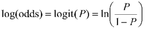
and captures the marginal distribution of the corresponding predicate.
Each formula can be associated with some weight value, that is a positive or negative real number. The higher the value of weight, the stronger the constraint represented by the formula. In contrast to classical logic, all worlds (i.e., Herbrand Interpretations) are possible with a certain probability [1]. The main idea behind this is that the probability of a world increases as the number of formulas it violates decreases.
Markov logic networks with its probabilistic approach combined to logic posit that a world is less likely if it violates formulas unlike in pure logic where a world is false if it violates even a single formula. Consider the case when a formula with high weight i.e. more significance is violated implying that it is less likely in occurrence.
Another important concept during the first phase of Weight Learning while applying an MLN template is “Grounding”. Grounding means to replace each variable/function in predicate with constants from the domain.
Weight Learning – An Example
Note: All examples are highlighted in the Alchemy MLN format
Let us consider an example where we want to identify the relationship between 2 different types of verb-noun pairs i.e noun subject and direct object.
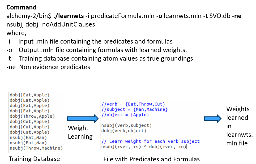
The input predicateFormula.mln file contains
- The predicates nsubj(verb, subject) and dobj(verb, object) and
- Formula of nsubj(+ver, +s) and dobj(+ver, +o)
These predicates or rules are to learn all possible SVO combinations i.e. what is the probability of a Subject-Verb-Object combination. The + sign ensures a cross product between the domains and learns all combinations. The training database consists of the nsubj and dobj tuples i.e. relations is the evidence used to learn the weights.
When we run the above command for this set of rules against the training evidence, we learn the weights as here:
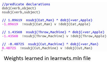
Note that the formula is now grounded by all occurrences of nsubj and dobj tuples from the training database or evidence and the weights are attached to it at the start of each such combination.
But it should be noted that there is no network yet and this is just a set of weighted first-order logic formulas. The MLN template we created so far will generate Markov networks from all of our ground formulas. Internally, it is represented as a factor graph.where each ground formula is a factor and all the ground predicates found in the ground formula are linked to the factor.
Inference
The definition goes as follows:
Estimate probability distribution encoded by a graphical model, for a given data (or observation).
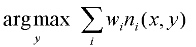
Out of the many Inference algorithms, the two major ones are MAP & Marginal Inference. For example, in a MAP Inference we find the most likely state of world given evidence, where y is the query and x is the evidence.
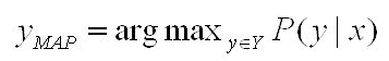
which is in turn equivalent to this formula.
Another is the Marginal Inference which computes the conditional probability of query predicates, given some evidence. Some advanced inference algorithms are Loopy Belief Propagation, Walk-SAT, MC-SAT, etc.
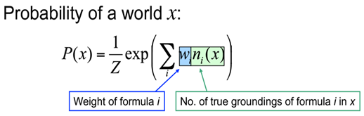
The probability of a world is given by the weighted sum of all true groundings of a formula i under an exponential function, divided by the partition function Z i.e. equivalent to the sum of the values of all possible assignments. The partition function acts a normalization constant to get the probability values between 0 and 1.
Inference – An Example
Let us draw inference on the the same example as earlier.
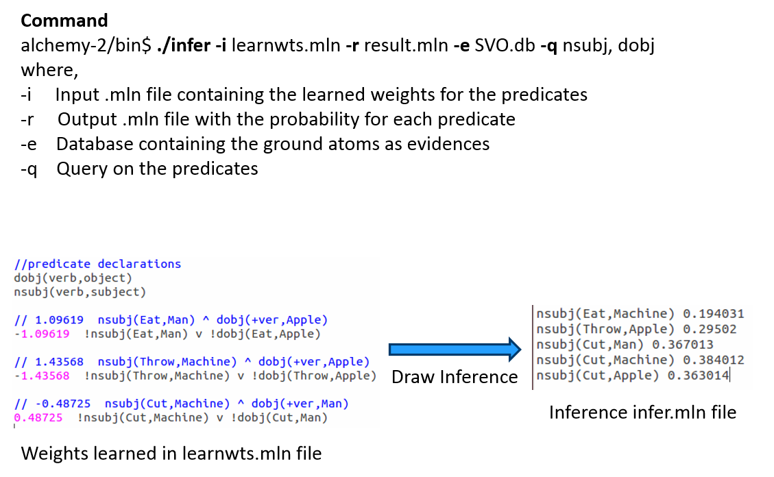
After learning the weights we run inference (with or without partial evidence) and query the relations of interest (nsubj here), to get inferred values.
Tool-kits
Let’s look at some of the MLN tool-kits at disposal to do learning and large scale inference. I have tried to make an assorted list of all tools here and tried to highlight some of its main features & problems.
For example, BUGS i.e. Bayesian Logic uses a Swift Compiler but is Not relational! ProbLog has a Python wrapper and is based on Horn clauses but has No Learning feature. These tools were invented in the initial days, much before the present day MLN looks like.
ProbCog developed at Technical University of Munich (TUM) & the AI Lab at Bremen covers not just MLN but also Bayesian Logic Networks (BLNs), Bayesian Networks & ProLog. In fact, it is now GUI based. Thebeast gives a shell to analyze & inspect model feature weights & missing features.
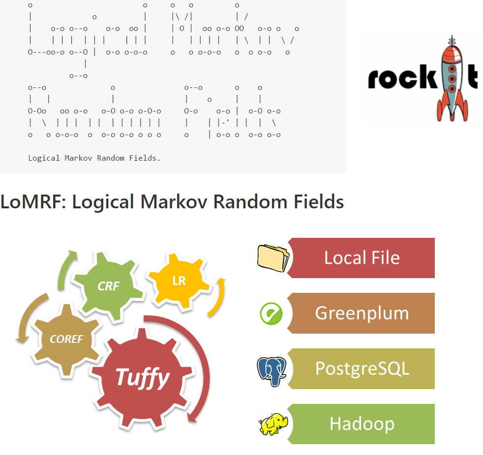
Alchemy from University of Washington (UoW) was the 1st First Order (FO) probabilistic logic toolkit. RockIt from University of Mannheim has an online & rest based interface and uses only Conjunctive Normal Forms (CNF) i.e. And-Or format in its formulas.
Tuffy scales this up by using a Relational Database Management System (RDBMS) whereas Felix allows Large Scale inference! Elementary makes use of secondary storage and Deep Dive is the current state of the art. All of these tools are part of the HAZY project group at Stanford University.
Lastly, LoMRF i.e. Logical Markov Random Field (MRF) is Scala based and has a feature to analyse different hypothesis by comparing the difference in .mln files!
Hope you enjoyed the read. The content starts from basic concepts and ends up highlighting key tools. In the final part of this 3 part blog series I would explain an application scenario and highlight the active research and industry players. Any feedback as a comment below or through a message is more than welcome!
Back to Part I – Statistical Relational Learning
Additional Links:
[1] Knowledge base files in Logical Markov Random Fields (LoMRF)
[2] (still) nothing clever Posts categorized “Machine Learning” – Markov Logic Networks
[3] A gentle introduction to statistical relational learning: maths, code, and examples