
Deep Autoregressive Models
In this blog article, we will discuss about deep autoregressive generative models (AGM). Autoregressive models were originated from economics and social science literature on time-series data where obser- vations from the previous steps are used to predict the value at the current and at future time steps [SS05]. Autoregression models can be expressed as:

where the terms  and
and  are constants to define the contributions of previous samples
  for the future value prediction. In the other words, autoregressive deep generative models are directed and fully observed models where outcome of the data completely depends on the previous data points as shown in Figure 1.
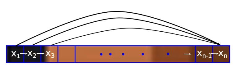
Figure 1: Autoregressive directed graph.
Let’s consider  , where
  is a set of images and each images is
  dimensional (n pixels). Then the prediction of new data pixel will be depending all the previously predicted pixels (Figure ?? shows the one row of pixels from an image). Referring to our last blog, deep generative models (DGMs) aim to learn the data distribution
  of the given training data and by following the chain rule of the probability, we can express it as:
(1) 
The above equation modeling the data distribution explicitly based on the pixel conditionals, which are tractable (exact likelihood estimation). The right hand side of the above equation is a complex distribution and can be represented by any possible distribution of  random variables. On the other hand, these kind of representation can have exponential space complexity. Therefore, in autoregressive generative models (AGM), these conditionals are approximated/parameterized by neural networks.
Training
As AGMs are based on tractable likelihood estimation, during the training process these methods maximize the likelihood of images over the given training data and it can be expressed as:
(2) 
The above expression is appearing because of the fact that DGMs try to minimize the distance between the distribution of the training data and the distribution of the generated data (please refer to our last blog). The distance between two distribution can be computed using KL-divergence:
(3) 
In the above equation the term  does not depend on
  , therefore, whole equation can be shortened to Equation 2, which represents the MLE (maximum likelihood estimation) objective to learn the model parameter by maximizing the log likelihood of the training images . From implementation point of view, the MLE objective can be optimized using the variations of stochastic gradient (ADAM, RMSProp, etc.) on mini-batches.
Network Architectures
As we are discussing deep generative models, here, we would like to discuss the deep aspect of AGMs. The parameterization of the conditionals mentioned in Equation 1 can be realized by different kind of network architectures. In the literature, several network architectures are proposed to increase their receptive fields and memory, allowing more complex distributions to be learned. Here, we are mentioning a couple of well known architectures, which are widely used in deep AGMs:
- Fully-visible sigmoid belief network (FVSBN): FVSBN is the simplest network without any hidden units and it is a linear combination of the input elements followed by a sigmoid function to keep output between 0 and 1. The positive aspects of this network is simple design and the total number of parameters in the model is quadratic which is much smaller compared to exponential [GHCC15].
- Neural autoregressive density estimator (NADE): To increase the effectiveness of FVSBN, the simplest idea would be to use one hidden layer neural network instead of logistic regression. NADE is an alternate MLP-based parameterization and more effective compared to FVSBN [LM11].
- Masked autoencoder density distribution (MADE): Here, the standard autoencoder neural networks are modified such that it works as an efficient generative models. MADE masks the parameters to follow the autoregressive property, where the current sample is reconstructed using previous samples in a given ordering [GGML15].
- PixelRNN/PixelCNN: These architecture are introducced by Google Deepmind in 2016 and utilizing the sequential property of the AGMs with recurrent and convolutional neural networks.
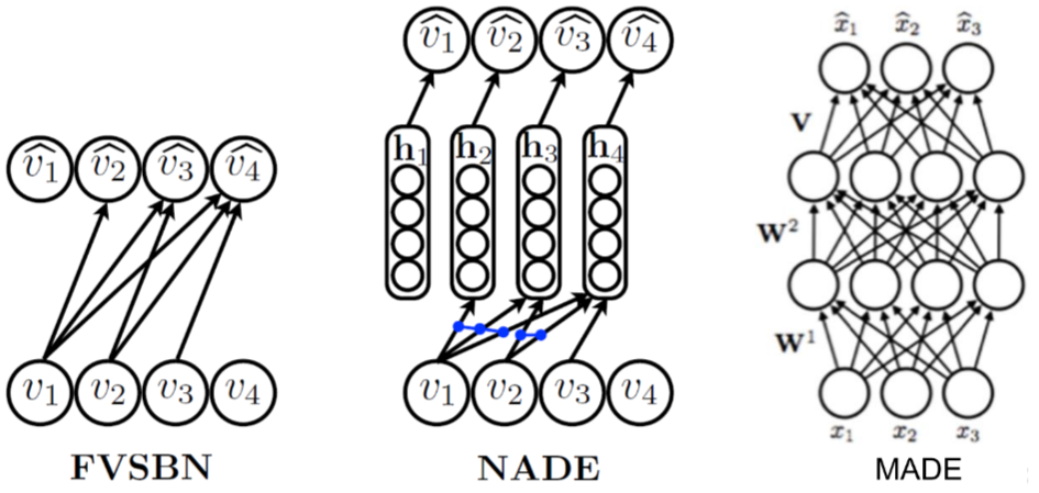
Figure 2: Different autoregressive architectures (image source from [LM11]).
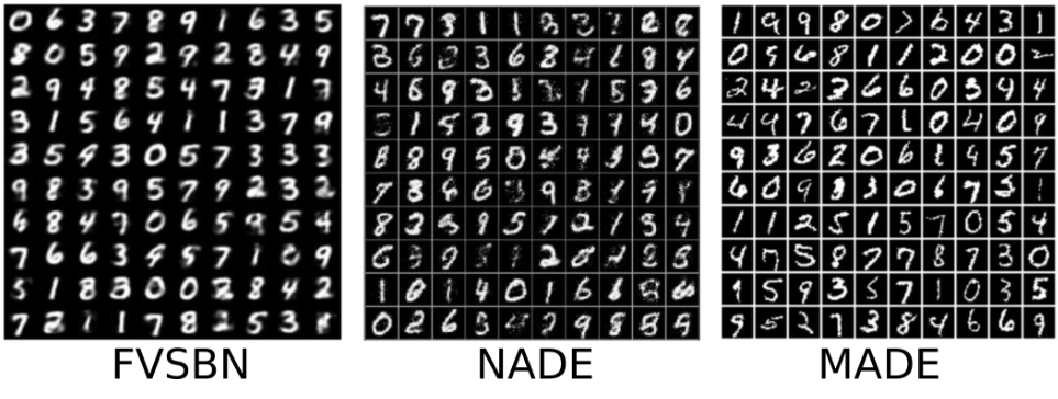
Results using different architectures (images source https://deepgenerativemodels.github.io).
It uses two different RNN architectures (Unidirectional LSTM and Bidirectional LSTM) to generate pixels horizontally and horizontally-vertically respectively. Furthermore, it ulizes residual connection to speed up the convergence and masked convolution to condition the different channels of images. PixelCNN applies several convolutional layers to preserve spatial resolution and increase the receptive fields. Furthermore, masking is applied to use only the previous pixels. PixelCNN is faster in training compared to PixelRNN. However, the outcome quality is better with PixelRNN [vdOKK16].
Summary
In this blog article, we discussed about deep autoregressive models in details with the mathematical foundation. Furthermore, we discussed about the training procedure including the summary of different network architectures. We did not discuss network architectures in details, we would continue the discussion of PixelCNN and its variations in upcoming blogs.
References
[GGML15] Mathieu Germain, Karol Gregor, Iain Murray, and Hugo Larochelle. MADE: masked autoencoder for distribution estimation. CoRR, abs/1502.03509, 2015.
[GHCC15] Zhe Gan, Ricardo Henao, David Carlson, and Lawrence Carin. Learning Deep Sigmoid Belief Networks with Data Augmentation. In Guy Lebanon and S. V. N. Vishwanathan, editors, Proceedings of the Eighteenth International Conference on Artificial Intelligence
and Statistics, volume 38 of Proceedings of Machine Learning Research, pages 268–276, San Diego, California, USA, 09–12 May 2015. PMLR.
[LM11] Hugo Larochelle and Iain Murray. The neural autoregressive distribution estimator. In Geoffrey Gordon, David Dunson, and Miroslav Dudík, editors, Proceedings of the Fourteenth International Conference on Artificial Intelligence and Statistics, volume 15 of Proceedings of Machine Learning Research, pages 29–37, Fort Lauderdale, FL, USA, 11–13 Apr 2011.
PMLR.
[SS05] Robert H. Shumway and David S. Stoffer. Time Series Analysis and Its Applications (Springer Texts in Statistics). Springer-Verlag, Berlin, Heidelberg, 2005.
[vdOKK16] A ̈aron van den Oord, Nal Kalchbrenner, and Koray Kavukcuoglu. Pixel recurrent neural
networks. CoRR, abs/1601.06759, 2016


Leave a Reply
Want to join the discussion?Feel free to contribute!