Tag Archive for: Machine Learning

Data-driven Attribution Modeling

In the world of commerce, companies often face the temptation to reduce their marketing spending, especially during times of economic uncertainty or when planning to cut costs. However, this short-term strategy can lead to long-term consequences that may hinder a company’s growth and competitiveness in the market.

Maintaining a consistent marketing presence is crucial for businesses, as it helps to keep the company at the forefront of their target audience’s minds. By reducing marketing efforts, companies risk losing visibility and brand awareness among potential clients, which can be difficult and expensive to regain later. Moreover, a strong marketing strategy is essential for building trust and credibility with prospective customers, as it demonstrates the company’s expertise, values, and commitment to their industry.

Given a fixed budget, companies apply economic principles for marketing efforts and need to spend a given marketing budget as efficient as possible. In this view, attribution models are an essential tool for companies to understand the effectiveness of their marketing efforts and optimize their strategies for maximum return on investments (ROI). By assigning optimal credit to various touchpoints in the customer journey, these models provide valuable insights into which channels, campaigns, and interactions have the greatest impact on driving conversions and therefore revenue. Identifying the most important channels enables companies to distribute the given budget accordingly in an optimal way.

1. Combining business value with attribution modeling

The true value of attribution modeling lies not solely in applying the optimal theoretical concept – that are discussed below – but in the practical application in coherence with the business logic of the firm. Therefore, the correct modeling ensures that companies are not only distributing their budget in an optimal way but also that they incorporate the business logic to focus on an optimal long-term growth strategy.

Understanding and incorporating business logic into attribution models is the critical step that is often overlooked or poorly understood. However, it is the key to unlocking the full potential of attribution modeling and making data-driven decisions that align with business goals. Without properly integrating the business logic, even the most sophisticated attribution models will fail to provide actionable insights and may lead to misguided marketing strategies.

Figure 1 – Combining the business logic with attribution modeling to generate value for firms

Figure 1 – Combining the business logic with attribution modeling to generate value for firms

For example, determining the end of a customer journey is a critical step in attribution modeling. When there are long gaps between customer interactions and touchpoints, analysts must carefully examine the data to decide if the current journey has concluded or is still ongoing. To make this determination, they need to consider the length of the gap in relation to typical journey durations and assess whether the gap follows a common sequence of touchpoints. By analyzing this data in an appropriate way, businesses can more accurately assess the impact of their marketing efforts and avoid attributing credit to touchpoints that are no longer relevant.

Another important consideration is accounting for conversions that ultimately lead to returns or cancellations. While it’s easy to get excited about the number of conversions generated by marketing campaigns, it’s essential to recognize that not all conversions should be valued equal. If a significant portion of conversions result in returns or cancellations, the true value of those campaigns may be much lower than initially believed.

To effectively incorporate these factors into attribution models, businesses need to important things. First, a robust data platform (such as a customer data platform; CDP) that can integrate data from various sources, such as tracking systems, ERP systems, e-commerce platforms to effectively perform data analytics. This allows for a holistic view of the customer journey, including post-conversion events like returns and cancellations, which are crucial for accurate attribution modeling. Second, as outlined above, businesses need a profound understanding of the business model and logic.

2. On the Relevance of Attribution Models in Online Marketing

A conversion is a point in the customer journey where a recipient of a marketing message performs a somewhat desired action. For example, open an email, click on a call-to-action link or go to a landing page and fill out a registration. Finally, the ultimate conversion would be of course buying the product. Attribution models serve as frameworks that help marketers assess the business impact of different channels on a customer’s decision to convert along a customer´s journey. By providing insights into which interactions most effectively drive sales, these models enable more efficient resource allocation given a fixed budget.

Figure 2 - A simple illustration of one single customer journey. Consider that from the company’s perspective all journeys together result into a complex network of possible journey steps.

Figure 2 – A simple illustration of one single customer journey. Consider that from the company’s perspective all journeys together result into a complex network of possible journey steps.

Companies typically utilize a diverse marketing mix, including email marketing, search engine advertising (SEA), search engine optimization (SEO), affiliate marketing, and social media. Attribution models facilitate the analysis of customer interactions across these touchpoints, offering a comprehensive view of the customer journey.

  • Comprehensive Customer Insights: By identifying the most effective channels for driving conversions, attribution models allow marketers to tailor strategies that enhance customer engagement and improve conversion rates.

  • Optimized Budget Allocation: These models reveal the performance of various marketing channels, helping marketers allocate budgets more efficiently. This ensures that resources are directed towards channels that offer the highest return on investment (ROI), maximizing marketing impact.

  • Data-Driven Decision Making: Attribution models empower marketers to make informed, data-driven decisions, leading to more effective campaign strategies and better alignment between marketing and sales efforts.

In the realm of online advertising, evaluating media effectiveness is a critical component of the decision-making process. Since advertisement costs often depend on clicks or impressions, understanding each channel’s effectiveness is vital. A multi-channel attribution model is necessary to grasp the marketing impact of each channel and the overall effectiveness of online marketing activities. This approach ensures optimal budget allocation, enhances ROI, and drives successful marketing outcomes.

What types of attribution models are there? Depending on the attribution model, different values are assigned to various touchpoints. These models help determine which channels are the most important and should be prioritized. Each channel is assigned a monetary value based on its contribution to success. This weighting then determines the allocation of the marketing budget. Below are some attribution models commonly used in marketing practice.

2.1. Single-Touch Attribution Models

As it follows from the name of the group of these approaches, they consider only one touchpoint.

2.1.1 First Touch Attribution

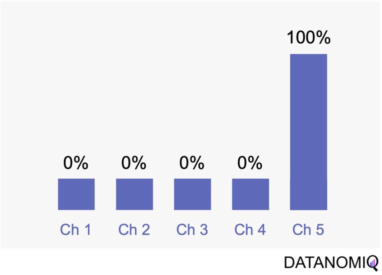
First touch attribution is the standard and simplest method for attributing conversions, as it assigns full credit to the first interaction. One of its main advantages is its simplicity; it is a straightforward and easy-to-understand approach. Additionally, it allows for quick implementation without the need for complex calculations or data analysis, making it a convenient choice for organizations looking for a simple attribution method. This model can be particularly beneficial when the focus is solely on demand generation. However, there are notable drawbacks to first touch attribution. It tends to oversimplify the customer journey by ignoring the influence of subsequent touchpoints. This can lead to a limited view of channel performance, as it may disproportionately credit channels that are more likely to be the first point of contact, potentially overlooking the contributions of other channels that assist in conversions.

Figure 3 - The first touch is a simple non-intelligent way of attribution.

Figure 3 – The first touch is a simple non-intelligent way of attribution.

2.1.2 Last Touch Attribution

Last touch attribution is another straightforward method for attributing conversions, serving as the opposite of first touch attribution by assigning full credit to the last interaction. Its simplicity is one of its main advantages, as it is easy to understand and implement without the need for complex calculations or data analysis. This makes it a convenient choice for organizations seeking a simple attribution approach, especially when the focus is solely on driving conversions. However, last touch attribution also has its drawbacks. It tends to oversimplify the customer journey by neglecting the influence of earlier touchpoints. This approach provides limited insights into the full customer journey, as it focuses solely on the last touchpoint and overlooks the cumulative impact of multiple touchpoints, missing out on valuable insights.

Figure 4 - Last touch attribution is the counterpart to the first touch approach.

Figure 4 – Last touch attribution is the counterpart to the first touch approach.

2.2 Multi-Touch Attribution Models

We noted that single-touch attribution models are easy to interpret and implement. However, these methods often fall short in assigning credit, as they apply rules arbitrarily and fail to accurately gauge the contribution of each touchpoint in the consumer journey. As a result, marketers may make decisions based on skewed data. In contrast, multi-touch attribution leverages individual user-level data from various channels. It calculates and assigns credit to the marketing touchpoints that have influenced a desired business outcome for a specific key performance indicator (KPI) event.

2.2.1 Linear Attribution

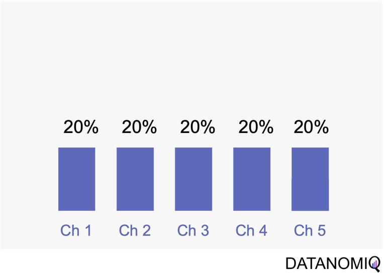
Linear attribution is a standard approach that improves upon single-touch models by considering all interactions and assigning them equal weight. For instance, if there are five touchpoints in a customer’s journey, each would receive 20% of the credit for the conversion. This method offers several advantages. Firstly, it ensures equal distribution of credit across all touchpoints, providing a balanced representation of each touchpoint’s contribution to conversions. This approach promotes fairness by avoiding the overemphasis or neglect of specific touchpoints, ensuring that credit is distributed evenly among channels. Additionally, linear attribution is easy to implement, requiring no complex calculations or data analysis, which makes it a convenient choice for organizations seeking a straightforward attribution method. However, linear attribution also has its drawbacks. One significant limitation is its lack of differentiation, as it assigns equal credit to each touchpoint regardless of their actual impact on driving conversions. This can lead to an inaccurate representation of the effectiveness of individual touchpoints. Furthermore, linear attribution ignores the concept of time decay, meaning it does not account for the diminishing influence of earlier touchpoints over time. It treats all touchpoints equally, regardless of their temporal proximity to the conversion event, potentially overlooking the greater impact of more recent interactions.

Figure 5 - Linear uniform attribution.

Figure 5 – Linear uniform attribution.

2.2.2 Position-based Attribution (U-Shaped Attribution & W-Shaped Attribution)

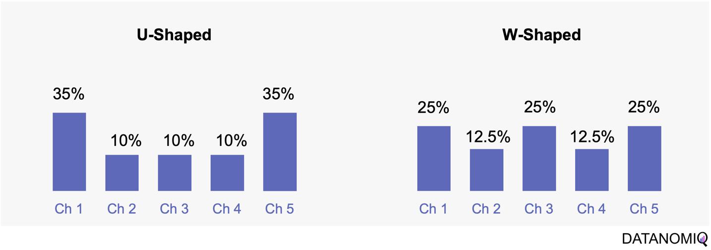
Position-based attribution, encompassing both U-shaped and W-shaped models, focuses on assigning the most significant weight to the first and last touchpoints in a customer’s journey. In the W-shaped attribution model, the middle touchpoint also receives a substantial amount of credit. This approach offers several advantages. One of the primary benefits is the weighted credit system, which assigns more credit to key touchpoints such as the first and last interactions, and sometimes additional key touchpoints in between. This allows marketers to highlight the importance of these critical interactions in driving conversions. Additionally, position-based attribution provides flexibility, enabling businesses to customize and adjust the distribution of credit according to their specific objectives and customer behavior patterns. However, there are some drawbacks to consider. Position-based attribution involves a degree of subjectivity, as determining the specific weights for different touchpoints requires subjective decision-making. The choice of weights can vary across organizations and may affect the accuracy of the attribution results. Furthermore, this model has limited adaptability, as it may not fully capture the nuances of every customer journey, given its focus on specific positions or touchpoints.

Figure 6 - The U-shaped attribution (sometimes known as "bathtube model" and the W-shaped one are first attempts of weighted models.

Figure 6 – The U-shaped attribution (sometimes known as “bathtube model” and the W-shaped one are first attempts of weighted models.

2.2.3 Time Decay Attribution

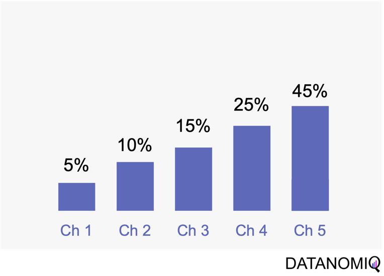
Time decay attribution is a model that primarily assigns most of the credit to interactions that occur closest to the point of conversion. This approach has several advantages. One of its key benefits is temporal sensitivity, as it recognizes the diminishing impact of earlier touchpoints over time. By assigning more credit to touchpoints closer to the conversion event, it reflects the higher influence of recent interactions. Additionally, time decay attribution offers flexibility, allowing organizations to customize the decay rate or function. This enables businesses to fine-tune the model according to their specific needs and customer behavior patterns, which can be particularly useful for fast-moving consumer goods (FMCG) companies. However, time decay attribution also has its drawbacks. One challenge is the arbitrary nature of the decay function, as determining the appropriate decay rate is both challenging and subjective. There is no universally optimal decay function, and choosing an inappropriate model can lead to inaccurate credit distribution. Moreover, this approach may oversimplify time dynamics by assuming a linear or exponential decay pattern, which might not fully capture the complex temporal dynamics of customer behavior. Additionally, time decay attribution primarily focuses on the temporal aspect and may overlook other contextual factors that influence touchpoint effectiveness, such as channel interactions, customer segments, or campaign-specific dynamics.

Figure 7 - Time-based models can be configurated by according to the first or last touch and weighted by the timespan in between of each touchpoint.

Figure 7 – Time-based models can be configurated by according to the first or last touch and weighted by the timespan in between of each touchpoint.

2.3 Data-Driven Attribution Models

2.3.1 Markov Chain Attribution

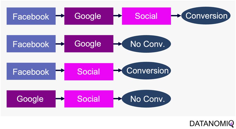
Markov chain attribution is a data-driven method that analyzes marketing effectiveness using the principles of Markov Chains. Those chains are mathematical models used to describe systems that transition from one state to another in a chain-like process. The principles focus on the transition matrix, derived from analyzing customer journeys from initial touchpoints to conversion or no conversion, to capture the sequential nature of interactions and understand how each touchpoint influences the final decision. Let’s have a look at the following simple example with three channels that are chained together and leading to either a conversion or no conversion.

Figure 8 - Example of four customer journeys

Figure 8 – Example of four customer journeys

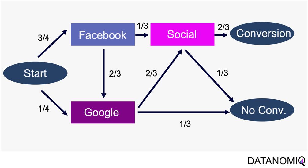
The model calculates the conversion likelihood by examining transitions between touchpoints. Those transitions are depicted in the following probability tree.

Figure 9 - Example of a touchpoint network based on customer journeys

Figure 9 – Example of a touchpoint network based on customer journeys

Based on this tree, the transition matrix can be constructed that reveals the influence of each touchpoint and thus the significance of each channel.

This method considers the sequential nature of customer journeys and relies on historical data to estimate transition probabilities, capturing the empirical behavior of customers. It offers flexibility by allowing customization to incorporate factors like time decay, channel interactions, and different attribution rules.

Markov chain attribution can be extended to higher-order chains, where the probability of transition depends on multiple previous states, providing a more nuanced analysis of customer behavior. To do so, the Markov process introduces a memory parameter 0 that is assumed to be zero here. Overall, it offers a robust framework for understanding the influence of different marketing touchpoints.

2.3.2 Shapley Value Attribution (Game Theoretical Approach)

The Shapley value is a concept from game theory that provides a fair method for distributing rewards among participants in a coalition. It ensures that both gains and costs are allocated equitably among actors, making it particularly useful when individual contributions vary but collective efforts lead to a shared outcome. In advertising, the Shapley method treats the advertising channels as players in a cooperative game. Now, consider a channel coalition consisting of different advertising channels . The utility function describes the contribution of a coalition of channels .

In this formula, is the cardinality of a specific coalition and the sum extends over all subsets of that do not contain the marginal contribution of channel to the coalition . For more information on how to calculate the marginal distribution, see Zhao et al. (2018).

The Shapley value approach ensures a fair allocation of credit to each touchpoint based on its contribution to the conversion process. This method encourages cooperation among channels, fostering a collaborative approach to achieving marketing goals. By accurately assessing the contribution of each channel, marketers can gain valuable insights into the performance of their marketing efforts, leading to more informed decision-making. Despite its advantages, the Shapley value method has some limitations. The method can be sensitive to the order in which touchpoints are considered, potentially leading to variations in results depending on the sequence of attribution. This sensitivity can impact the consistency of the outcomes. Finally, Shapley value and Markov chain attribution can also be combined using an ensemble attribution model to further reduce the generalization error (Gaur & Bharti 2020).

2.33. Algorithmic Attribution using binary Classifier and (causal) Machine Learning

While customer journey data often suffices for evaluating channel contributions and strategy formulation, it may not always be comprehensive enough. Fortunately, companies frequently possess a wealth of additional data that can be leveraged to enhance attribution accuracy by using a variety of analytics data from various vendors. For examples, companies might collect extensive data, including customer website activity such as clicks, page views, and conversions. This data includes features like for example the Urchin Tracking Module (UTM) information such as source, medium, campaign, content and term as well as campaign, device type, geographical information, number of user engagements, and scroll frequency, among others.

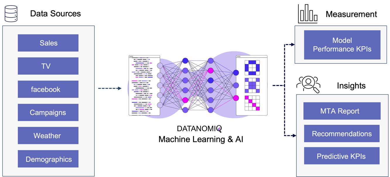
Utilizing this information, a binary classification model can be trained to predict the probability of conversion at each step of the multi touch attribution (MTA) model. This approach not only identifies the most effective channels for conversions but also highlights overvalued channels. Common algorithms include logistic regressions to easily predict the probability of conversion based on various features. Gradient boosting also provides a popular ensemble technique that is often used for unbalanced data, which is quite common in attribution data. Moreover, random forest models as well as support vector machines (SVMs) are also frequently applied. When it comes to deep learning models, that are often used for more complex problems and sequential data, Long Short-Term Memory (LSTM) networks or Transformers are applied. Those models can capture the long-range dependencies among multiple touchpoints.

Figure 10 - Attribution Model based on Deep Learning / AI

Figure 10 – Attribution Model based on Deep Learning / AI

The approach is scalable, capable of handling large volumes of data, making it ideal for organizations with extensive marketing campaigns and complex customer journeys. By leveraging advanced algorithms, it offers more accurate attribution of credit to different touchpoints, enabling marketers to make informed, data-driven decisions.

All those models are part of the Machine Learning & AI Toolkit for assessing MTA. And since the business world is evolving quickly, newer methods such as double Machine Learning or causal forest models that are discussed in the marketing literature (e.g. Langen & Huber 2023) in combination with eXplainable Artificial Intelligence (XAI) can also be applied as well in the DATANOMIQ Machine Learning and AI framework.

3. Conclusion

As digital marketing continues to evolve in the age of AI, attribution models remain crucial for understanding the complex customer journey and optimizing marketing strategies. These models not only aid in effective budget allocation but also provide a comprehensive view of how different channels contribute to conversions. With advancements in technology, particularly the shift towards data-driven and multi-touch attribution models, marketers are better equipped to make informed decisions that enhance quick return on investment (ROI) and maintain competitiveness in the digital landscape.

Several trends are shaping the evolution of attribution models. The increasing use of machine learning in marketing attribution allows for more precise and predictive analytics, which can anticipate customer behavior and optimize marketing efforts accordingly. Additionally, as privacy regulations become more stringent, there is a growing focus on data quality and ethical data usage (Ethical AI), ensuring that attribution models are both effective and compliant. Furthermore, the integration of view-through attribution, which considers the impact of ad impressions that do not result in immediate clicks, provides a more holistic understanding of customer interactions across channels. As these models become more sophisticated, they will likely incorporate a wider array of data points, offering deeper insights into the customer journey.

Unlock your marketing potential with a strategy session with our DATANOMIQ experts. Discover how our solutions can elevate your media-mix models and boost your organization by making smarter, data-driven decisions.

References

  • Zhao, K., Mahboobi, S. H., & Bagheri, S. R. (2018). Shapley value methods for attribution modeling in online advertising. arXiv preprint arXiv:1804.05327.
  • Gaur, J., & Bharti, K. (2020). Attribution modelling in marketing: Literature review and research agenda. Academy of Marketing Studies Journal, 24(4), 1-21.
  • Langen H, Huber M (2023) How causal machine learning can leverage marketing strategies: Assessing and improving the performance of a coupon campaign. PLoS ONE 18(1): e0278937. https://doi.org/10.1371/journal. pone.0278937

How to speed up claims processing with automated car damage detection

AI drives automation, not only in industrial production or for autonomous driving, but above all in dealing with bureaucracy. It is an realy enabler for lean management!

One example is the use of Deep Learning (as part of Artificial Intelligence) for image object detection. A car insurance company checks the amount of the damage by a damage report after car accidents. This process is actually performed by human professionals. With AI, we can partially automate this process using image data (photos of car damages). After an AI training with millions of photos in relation to real costs for repair or replacement, the cost estimation gets suprising accurate and supports the process in speed and quality.

AI drives automation and DATANOMIQ drives this automation with you! You can download the Infographic as PDF.

How to speed up claims processing with automated car damage detection

How to speed up claims processing
with automated car damage detection

Download this Infographic as PDF now by clicking here!

We wrote this article in cooperation with pixolution, a company for computer vision and AI-bases visual search. Interested in introducing AI / Deep Learning to your organization? Do not hesitate to get in touch with us!

DATANOMIQ is the independent consulting and service partner for business intelligence, process mining and data science. We are opening up the diverse possibilities offered by big data and artificial intelligence in all areas of the value chain. We rely on the best minds and the most comprehensive method and technology portfolio for the use of data for business optimization.

Data Dimensionality Reduction Series: Random Forest

Hello lovely individuals, I hope everyone is doing well, is fantastic, and is smiling more than usual. In this blog we shall discuss a very interesting term used to build many models in the Data science industry as well as the cyber security industry.

SUPER BASIC DEFINITION OF RANDOM FOREST:

Random forest is a form of Supervised Machine Learning Algorithm that operates on the majority rule. For example, if we have a number of different algorithms working on the same issue but producing different answers, the majority of the findings are taken into account. Random forests, also known as random selection forests, are an ensemble learning approach for classification, regression, and other problems that works by generating a jumble of decision trees during training.

When it comes to regression and classification, random forest can handle both categorical and continuous variable data sets. It typically helps us outperform other algorithms and overcome challenges like overfitting and the curse of dimensionality.

QUICK ANALOGY TO UNDERSTAND THINGS BETTER:

Uncle John wants to see a doctor for his acute abdominal discomfort, so he goes to his pals for recommendations on the top doctors in town. After consulting with a number of friends and family members, Atlas chooses to visit the doctor who received the highest recommendations.

So, what does this mean? The same is true for random forests. It builds decision trees from several samples and utilises their majority vote for classification and average for regression.

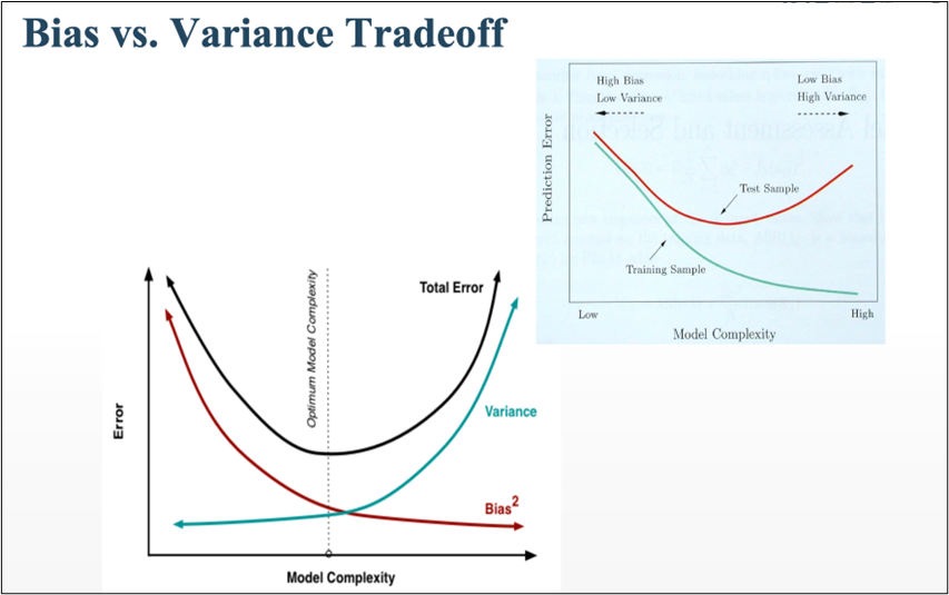
HOW BIAS AND VARIANCE AFFECTS THE ALGORITHM?

  1. BIAS
  • The algorithm’s accuracy or quality is measured.
  • High bias means a poor match
  1. VARIANCE
  • The accuracy or specificity of the match is measured.
  • A high variance means a weak match

We would like to minimise each of these. But, unfortunately we can’t do this independently, since there is a trade-off

EXPECTED PREDICTION ERROR = VARIANCE + BIAS^2 + NOISE^2

Bias vs Variance Tradeoff

HOW IS IT DIFFERENT FROM OTHER TWO ALGORITHMS?

Every other data dimensionality reduction method, such as missing value ratio and principal component analysis, must be built from the scratch, but the best thing about random forest is that it comes with built-in features and is a tree-based model that uses a combination of decision trees for non-linear data classification and regression.

Without wasting much time, let’s move to the main part where we’ll discuss the working of RANDOM FOREST:

WORKING WITH RANDOM FOREST:

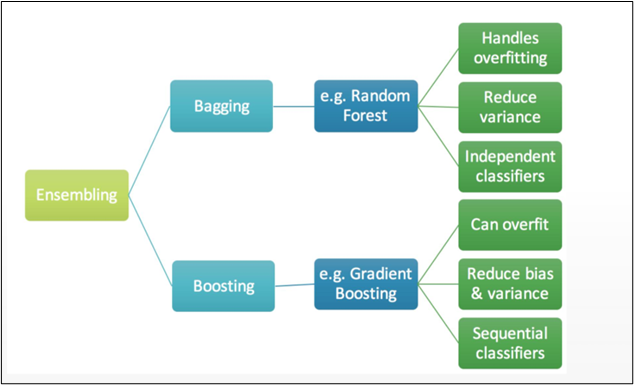
As we saw in the analogy, RANDOM FOREST operates on the basis of ensemble technique; however, what precisely does ensemble technique mean? It’s actually rather straightforward. Ensemble simply refers to the combination of numerous models. As a result, rather than a single model, a group of models is utilised to create predictions.

ENSEMBLE TECHNIQUE HAS 2 METHODS:

Ensemble Learning: Bagging and Boosting

1] BAGGING

2] BOOSTING

Let’s dive deep to understand things better:

1] BAGGING:

LET’S UNDERSTAND IT THROUGH A BETTER VIEW:

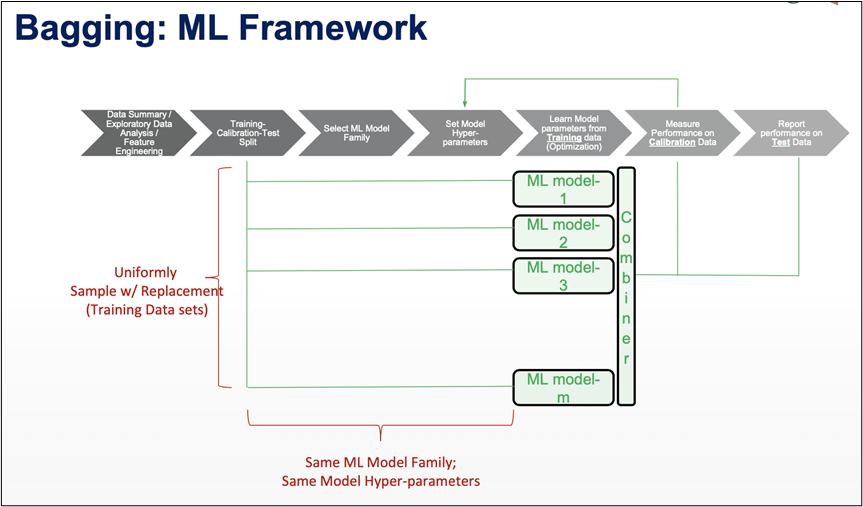
Bagging simply helps us to reduce the variance in a loud datasets. It works on an ensemble technique.

  1. Algorithm independent : general purpose technique
  2. Well suited for high variance algorithms
  3. Variance reduction is achieved by averaging a group of data.
  4. Choose # of classifiers to build (B)

DIFFERENT TRAINING DATA:

  1. Sample Training Data with Replacement
  2. Same algorithm on different subsets of training data

APPLICATION :

  1. Use with high variance algorithms (DT, NN)
  2. Easy to parallelize
  3. Limitation: Loss of Interpretability
  4. Limitation: What if one of the features dominates?

SUMMING IT ALL UP:

  1. Ensemble approach = Bootstrap Aggregation.
  2. In bagging a random dataset is selected as shown in the above figure and then a model is built using those random data samples which is termed as bootstrapping.
  3. Now, when we train this random sample data it is not mendidate to select data points only once, while training the sample data we can select the individual data point more then once.
  4. Now each of these models is built and trained and results are obtained.
  5. Lastly the majority results are being considered.

We can even calculate  the error from this thing know as random forest OOB error:

RANDOM FORESTS: OOB ERROR  (Out-of-Bag Error) :

▪ From each bootstrapped sample, 1/3rd of it is kept aside as “Test”

▪ Tree built on remaining 2/3rd

▪ Average error from each of the “Test” samples is called “Out-of-Bag Error”

▪ OOB error provides a good estimate of model error

▪ No need for separate cross validation

2] BOOSTING:

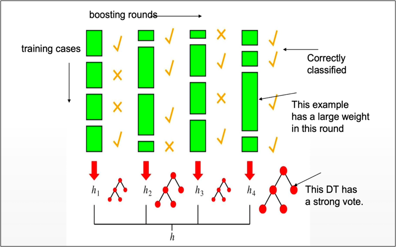
Boosting in short helps us to improve our prediction by reducing error in predictive data analysis.

Weak Learner: only needs to generate a hypothesis with a training accuracy greater than 0.5, i.e., < 50% error over any distribution.

KEY INTUITION:

  1. Strong learners are very difficult to construct
  2. Constructing weaker Learners is relatively easy influence with the empirical squared improvement when assigned to the model

APPROACH OUTLINE:

  1. Start with a ML algorithm for finding the rough rules of thumb (a.k.a. “weak” or “base” algorithm)
  2. Call the base algorithm repeatedly, each time feeding it a different subset of the training examples
  3. The basic learning algorithm creates a new weak prediction rule each time it is invoked.
  4. After several rounds, the boosting algorithm must merge these weak rules into a single prediction rule that, hopefully, is considerably more accurate than any of the weak rules alone.

TWO KEY DETAILS :

  1. In each round, how is the distribution selected ?
  2. What is the best way to merge the weak rules into a single rule?

BOOSTING is classified into two types:

1] ADA BOOST

2] XG BOOST

As far as the Random forest is concerned it is said that it follows the bagging method, not a boosting method. As the name implies, boosting involves learning from others, which in turn increases learning. Random forests have trees that run in parallel. While creating the trees, there is no interaction between them.

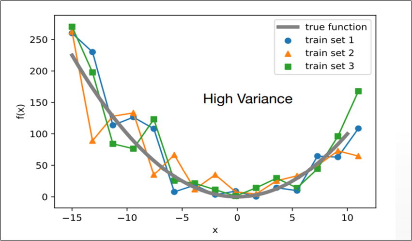
Boosting helps us reduce the error by decreasing the bias whereas, on other hand, Bagging is a manner to decrease the variance within the prediction with the aid of generating additional information for schooling from the dataset using mixtures with repetitions to provide multi-sets of the original information.

How Bagging helps with variance – A Simple Example

BAGGED TREES

  1. Decision Trees have high variance
  2. The resultant tree (model) is determined by the training data.
  3. (Unpruned) Decision Trees tend to overfit
  4. One option: Cost Complexity Pruning

BAG TREES

  1. Sample with replacement (1 Training set → Multiple training sets)
  2. Train model on each bootstrapped training set
  3. Multiple trees; each different : A garden ☺
  4. Each DT predicts; Mean / Majority vote prediction
  5. Choose # of trees to build (B)

ADVANTAGES

Reduce model variance / instability.

RANDOM FOREST : VARIABLE IMPORTANCE

VARIABLE IMPORTANCE :

▪ Each time a tree is split due to a variable m, Gini impurity index of the parent node is higher than that of the child nodes

▪ Adding up all Gini index decreases due to variable m over all trees in the forest, gives a measure of variable importance

IMPORTANT FEATURES AND HYPERPARAMETERS:

  1. Diversity :
  2. Immunity to the curse of dimensionality :
  3. Parallelization :
  4. Train-Test split :
  5. Stability :
  6. Gini significance (or mean reduction impurity) :
  7. Mean Decrease Accuracy :

FEATURES THAT IMPROVE THE MODEL’S PREDICTIONS and SPEED :

  1. maximum_features :

Increasing max features often increases model performance since each node now has a greater number of alternatives to examine.

  1. n_estimators :

The number of trees you wish to create before calculating the maximum voting or prediction averages. A greater number of trees improves speed but slows down your code.

  1. min_sample_leaf :

If you’ve ever designed a decision tree, you’ll understand the significance of the minimal sample leaf size. A leaf is the decision tree’s last node. A smaller leaf increases the likelihood of the model collecting noise in train data.

  1. n_jobs :

This option instructs the engine on how many processors it is permitted to utilise.

  1. random_state :

This argument makes it simple to duplicate a solution. If given the same parameters and training data, a definite value of random state will always provide the same results.

  1. oob_score:

A random forest cross validation approach is used here. It is similar to the leave one out validation procedure, except it is significantly faster.

LET’S SEE THE STEPS INVOLVED IN IMPLEMENTATION OF RANDOM FOREST ALGORITHM:

Step1: Choose T- number of trees to grow

Step2: Choose m<p (p is the number of total features) —number of features used to calculate the best split at each node (typically 30% for regression, sqrt(p) for classification)

Step3: For each tree, choose a training set by choosing N times (N is the number of training examples) with replacement from the training set

Step4: For each node, calculate the best split, Fully grown and not pruned.

Step5: Use majority voting among all the trees

Following is a full case study and implementation of all the principles we just covered, in the form of a jupyter notebook including every concept and all you ever wanted to know about RANDOM FOREST.

GITHUB Repository for this blog article: https://gist.github.com/Vidhi1290/c9a6046f079fd5abafb7583d3689a410

AI for games, games for AI

1, Who is playing or being played?

Since playing Japanese video games named “Demon’s Souls” and “Dark Souls” when they were released by From Software, I had played almost no video games for many years. During the period, From Software established one genre named soul-like games. Soul-like games are called  死にゲー in Japanese, which means “dying games,” and they are also called マゾゲー, which means “masochistic games.”  As the words imply, you have to be almost masochistic to play such video games because you have to die numerous times in them. And I think recently it has been one of the most remarkable times for From Software because in November of 2021 “Dark Souls” was selected the best video game ever by Golden Joystick Awards. And in the end of last February a new video game by From Software called “Elden Ring” was finally released. After it proved that Miyazaki Hidetaka, the director of Soul series, collaborated with George RR Martin, the author of the original of “Game of Thrones,” “Elden Ring” had been one of the most anticipated video games. In spite of its notorious difficulty as well as other soul-like games so far, “Elden Ring” became a big hit, and I think Miyazak Hidetaka is now the second most famous Miyazaki in the world.  A lot of people have been playing it, raging, and screaming. I was no exception, and it took me around 90 hours to finish the video game, breaking a game controller by the end of it. It was a long time since I had been so childishly emotional last time, and I was almost addicted to trial and errors the video game provides. At the same time, one question crossed my mind: is it the video game or us that is being played?

The childhood nightmare strikes back. Left: the iconic and notorious boss duo Ornstein and Smough in Dark Souls (2011), right: Godskin Duo in Elden Ring (2022).

Miyazaki Hidetaka entered From Software in 2004 and in the beginning worked as a programmer of game AI, which controls video games in various ways. In the same year an AI researcher Miyake Youichiro also joined From Software, and I studied a little about game AI by his book after playing “Elden Ring.” I found that he also joined “Demon’s Souls,” in which enemies with merciless game AI were arranged, and I had to conquer them to reach the demon in the end at every dungeon. Every time I died, even in the terminal place with the boss fight, I had to restart from the start, with all enemies reviving. That requires a lot of trial and errors, and that was the beginning of soul-like video games today.  In the book by the game AI researcher who was creating my tense and almost traumatizing childhood experiences, I found that very sophisticated techniques have been developed to force players to do trial and errors. They were sophisticated even at a level of controlling players at a more emotional level. Even though I am familiar with both of video games and AI at least more than average, it was not until this year that I took care about this field. After technical breakthroughs mainly made Western countries, video game industry showed rapid progress, and industry is now a huge entertainment industry, whose scale is now bigger that those of movies and music combined. Also the news that Facebook changed its named to Meta and that Microsoft announced to buy Activision Blizzard were sensational recently. However media coverage about those events would just give you impressions that those giant tech companies are making uses of the new virtual media as metaverse or new subscription services. At least I suspect these are juts limited sides of investments on the video game industry.

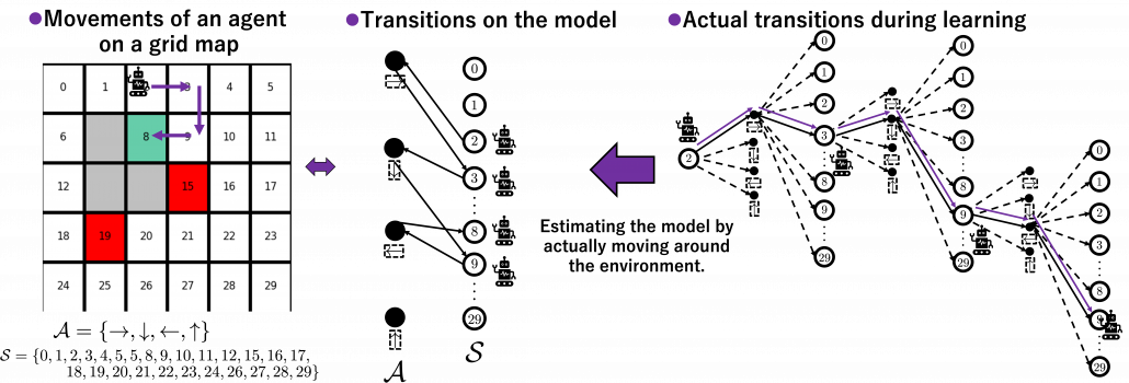
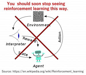
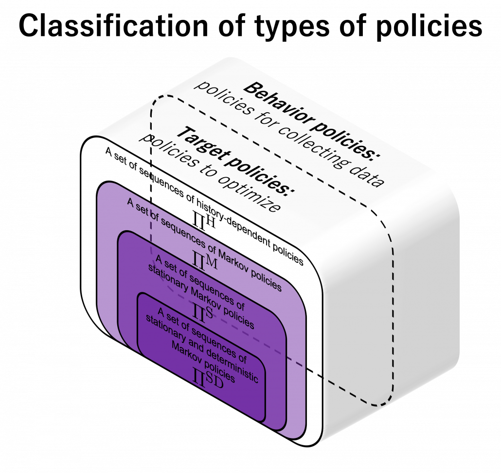
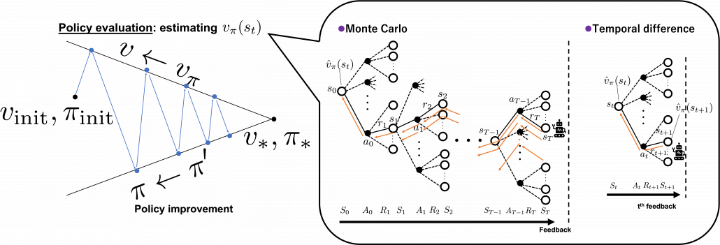
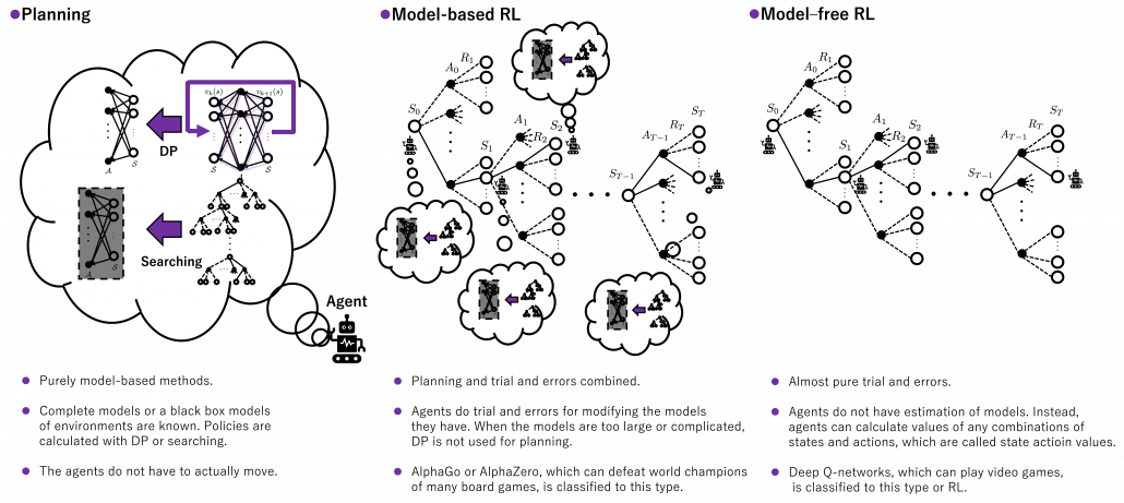
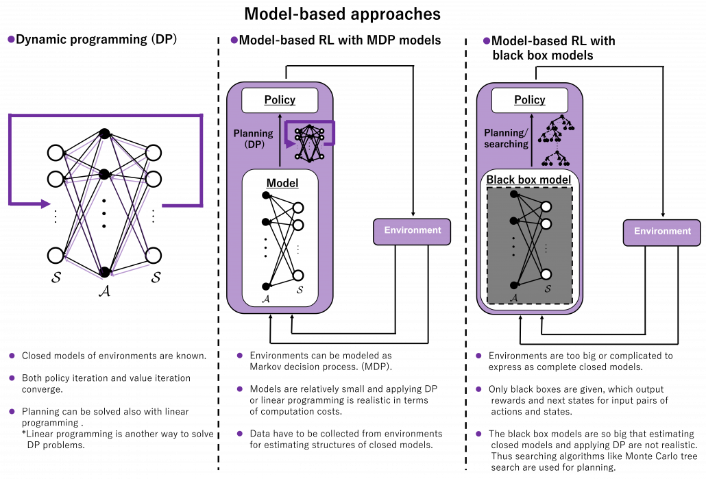
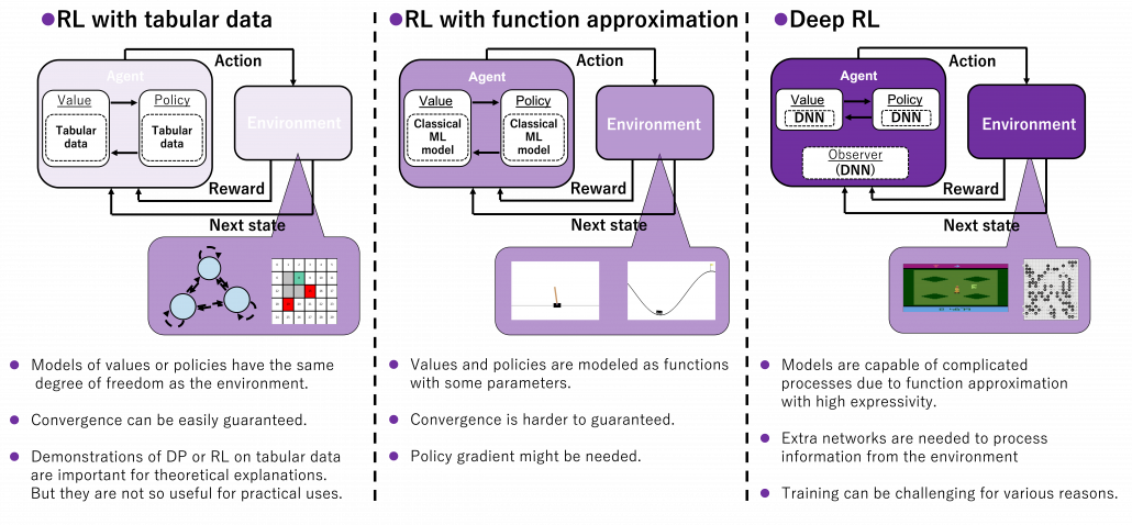
The book on game AI also made me rethink AI technologies also because I am currently writing an article series on reinforcement learning (RL) as a kind of my study note. RL is a type of training of an AI agent through trial-and-error-like processes. Rather than a labeled dataset, RL needs an environment. Such environment receives an action from an agent and gives the consequent state and next reward. From a view point of the agent, it give an action and gets the consequent next state and a corresponding reward, which looks like playing a video game. RL mainly considers a more simplified version of video-game-like environments called a Markov decision processes (MDPs), and in an MDP at a time step t an RL agents takes an action A_t, and gets the next state S_t and a corresponding reward R_t. An MDP is often displayed as a graph at the left side below or the graphical model at the right side.

Compared to a normal labeled dataset used for other machine learning, such environment is something hard to prepare. The video game industry has been a successful manufacturer of such environments, and as a matter of fact video games of Atari or Nintendo Entertainment System (NES) are used as benchmarks of theoretical papers on RL. Such video games might be too primitive for considering practical uses, but researches on RL are little by little tackling more and more complicated video games or simulations. But also I am sure creating AI that plays video games better than us would not be their goals. The situation seems like they are cultivating a form of more general intelligence inside computer simulations which is also effective to the real world. Someday, experiences or intelligence grown in such virtual reality might be dragged to our real world.

Testing systems in simulations has been a fascinating idea, and that is also true of AI research. As I mentioned, video games are frequently used to evaluate RL performances, and there are some tools for making RL environments with modern video game engines. Providing a variety of such sophisticated computer simulations will be indispensable for researches on AI. RL models need to be trained in simulations before being applied on physical devices because most real machines would not endure numerous trial and errors RL often requires. And I believe the video game industry has a potential of developing such experimental fields of AI fueled by commercial success in entertainment. I think the ideas of testing systems or training AI in simulations is getting a bit more realistic due to recent development of transfer learning.

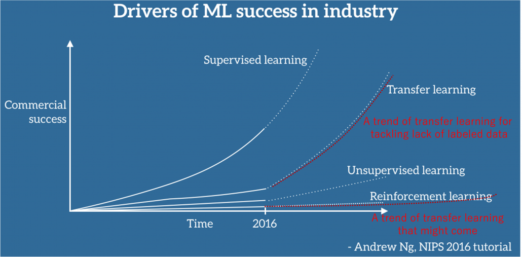
Transfer learning is a subfield of machine learning which apply intelligence or experiences accumulated in datasets or tasks to other datasets or tasks. This is not only applicable to RL but also to more general machine learning tasks like regression or classification. Or rather it is said that transfer learning in general machine learning would show greater progress at a commercial level than RL for the time being. And transfer learning techniques like using pre-trained CNN or BERT is already attracting a lot of attentions. But I would say this is only about a limited type of transfer learning. According to Matsui Kota in RIKEN AIP Data Driven Biomedical Science Team, transfer learning has progressed rapidly after the advent of deep learning, but many types of tasks and approaches are scattered in the field of transfer learning. As he says, the term transfer learning should be more carefully used. I would like to say the type of transfer learning discussed these days are a family of approaches for tackling lack of labels. At the same time some of current researches on transfer learning is also showing possibilities that experiences or intelligence in computer simulations are transferable to the real world. But I think we need to wait for more progress in RL before such things are enabled.
In this article I would like to explain how video games or computer simulations can provide experiences to the real world in two ways. I am first going to briefly explain how video game industry in the first place has been making game AI to provide game users with tense experiences. And next I will explain how RL has become a promising technique to beat such games which were originally invented to moderately harass human players. And in the end, I am going to briefly introduce ideas of transfer learning applicable to video games or computer simulations. What I can talk in this article is very limited for these huge study areas or industries. But I hope you would see the video game industry and transfer learning in different ways after reading this article, and that might give you some hints about how those industries interact to each other in the future. And also please keep it in mind that I am not going to talk so much about growing video game markets, computer graphics, or metaverse. Here I focus on aspects of interweaving knowledge and experiences generated in simulation or real physical worlds.

2, Game AI

The fact that “Dark Souls” was selected the best game ever at least implies that current video game industry makes much of experiences of discoveries and accomplishments while playing video games, rather than cinematic and realistic computer graphics or iconic and world widely popular characters. That is a kind of returning to the origin of video games. Video games used to be just hard because the more easily players fail, the more money they would drop in arcade games. But I guess this aspect of video games tend to be missed when you talk about video games as a video game fan. What you see in advertisements of video games are more of beautiful graphics, a new world, characters there, and new gadgets. And it has been actually said that qualities of computer graphics have a big correlation with video game sales. In the third article of my series on recurrent neural networks (RNN), I explained how video game industry laid a foundation of the third AI boom during the second AI winter in 1990s. To be more concrete, graphic cards developed rapidly to realize more photo realistic graphics in PC games, and the graphic card used in Xbox was one of the first programmable GPU for commercial uses. But actually video games developed side by side with computer science also outside graphics. Thus in this section I am going to how video games have developed by focusing on game AI, which creates intelligence in video games in several ways. And my explanations on game AI is going to be a rough introduction to a huge and great educational works by Miyake Youichiro.

Playing video games is made up by decision makings, and such decision makings are made in react to game AI. In other words, a display is input into your eyes or sight nerves, and sequential decision makings, that is how you have been moving fingers are outputs. Complication of the experiences, namely hardness of video games, highly depend on game AI.  Game AI is mainly used to design enemies in video games to hunt down players. Ideally game AI has to be both rational and human. Rational game AI implemented in enemies frustrate or sometimes despair users by ruining users’ efforts to attack them, to dodge their attacks, or to use items. At the same time enemies have to retain some room for irrationality, that is they have to be imperfect. If enemies can perfectly conquer players’ efforts by instantly recognizing their commands, such video games would be theoretically impossible to beat. Trying to defeat such enemies is nothing but frustrating. Ideal enemies let down their guard and give some timings for attacking and trying to conquer them. Sophisticated game AI is inevitable to make grownups all over the world childishly emotional while playing video games.

These behaviors of game AI are mainly functions of character AI, which is a part of game AI. In order to explain game AI, I also have to explain a more general idea of AI, which is not the one often called “AI” these days. Artificial intelligence (AI) is in short a family of technologies to create intelligence, with computers. And AI can be divided into two types, symbolism AI and connectionism AI. Roughly speaking, the former is manual and the latter is automatic. Symbolism AI is described with a lot of rules, mainly “if” or “else” statements in code. For example very simply “If the score is greater than 5, the speed of the enemy is 10.” Or rather many people just call it “programming.”

*Note that in contexts of RL, “game AI” often means AI which plays video games or board games. But “game AI” in video games is a more comprehensive idea orchestrating video games.
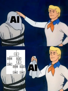
This meme describes symbolism AI well.

What people usually call “AI” in this 3rd AI boom is the latter, connictionism AI. Connectionism AI basically means neural networks, which is said to be inspired by connections of neurons. But the more you study neural networks, the more you would see such AI just as “functions capable of universal approximation based on data.” That means, a function f, which you would have learned in school such as y = f(x) = ax + b is replaced with a complicated black box, and such black box f is automatically learned with many combinations of (x, y). And such black boxes are called neural networks, and the combinations of (x, y) datasets. Connectionism AI might sound more ideal, but in practice it would be hard to design characters in AI based on such training with datasets.

*Connectionism, or deep learning is of course also programming. But in deep learning we largely depend on libraries, and a lot of parameters of AI models are updated automatically as long as we properly set datasets. In that sense, I would connectionism is more automatic. As I am going to explain, game AI largely depends on symbolism AI, namely manual adjustment of lesser parameters, but such symbolism AI would behave much more like humans than so called “AI” these days when you play video games.

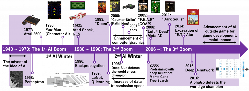
Digital game AI today is application of the both types of AI in video games. It initially started mainly with symbolism AI till around 2010, and as video games get more and more complicated connectionism AI are also introduced in game AI. Video game AI can be classified to mainly navigation AI, character AI, meta AI, procedural AI, and AI outside video games. The figure below shows relations of general AI and types of game AI.
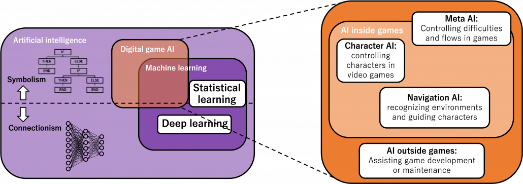
Very simply putting, video game AI traced a history like this: the initial video games were mainly composed of navigation AI showing levels, maps, and objects which move deterministically based on programming.  Players used to just move around such navigation AI. Sooner or later, enemies got certain “intelligence” and learned to chase or hunt down players, and that is the advent of character AI. But of course such “intelligence” is nothing but just manual programs. After rapid progress of video games and their industry, meta AI was invented to control difficulties of video games, thereby controlling players’ emotions. Procedural AI automatically generates contents of video games, so video games are these days becoming more and more massive. And as modern video games are too huge and complicated to debug or maintain manually, AI technologies including deep learning are used. The figure below is a chronicle of development of video games and AI technologies covered in this article. Let’s see a brief history of video games and game AI by taking a closer look at each type of game AI a little more precisely.
Navigation AI

Navigation AI is the most basic type of game AI, and that allows character AI to recognize the world in video games. Even though I think character AI, which enables characters in video games to behave like humans, would be the most famous type of game AI, it is said navigation AI has an older history. One important function of navigation AI is to control objects in video games, such as lifts, item blocks, including attacks by such objects. The next aspect of navigation AI is that it provides character AI with recognition of worlds. Unlike humans, who can almost instantly roughly recognize circumstances, character AI cannot do that as we do. Even if you feel as if the character you are controlling are moving around mountains, cities, or battle fields, sometimes escaping from attacks by other AI, for character AI that is just moving on certain graphs. The figure below are some examples of world representations adopted in some popular video games. There are a variety of such representations, and please let me skip explaining the details of them. An important point is, relatively wide and global recognition of worlds by characters in video games depend on how navigation AI is designed.
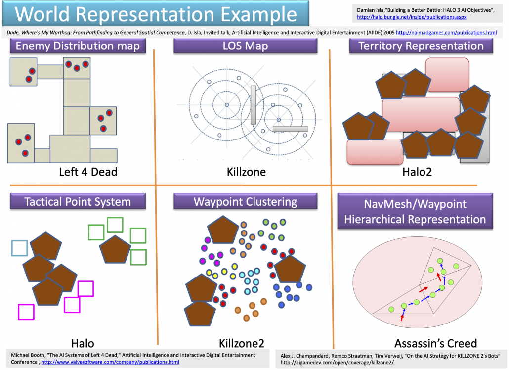
The next important feature of navigation AI is path finding. If you have learned engineering or programming, you should be already familiar with pathfiniding algorithms. They had been known since a long time ago, but it was not until “Counter-Strike” in 2000 the techniques were implemented at an satisfying level for navigating characters in a 3d world. Improvements of pathfinding in video games released game AI from fixed places and enabled them to be more dynamic.

*According to Miyake Youichiro, the advent of pathfinding in video games released character AI from staying in a narrow space and enable much more dynamic and human-like movements of them. And that changed game AI from just static objects to more intelligent entity.
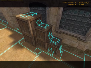
Navigation meshes in “Counter-Strike (2000).” Thanks to these meshes, continuous 3d world can be processed as discrete nodes of graphs.

Character AI

Character AI is something you would first imagine from the term AI. It controls characters’ actions in video games. And differences between navigation AI and character AI can be ambiguous. It is said Pac-Man is one of the very first character AI. Compared to aliens in Space Invader deterministically moved horizontally, enemies in Pac-Man chase a player, and this is the most straightforward difference between navigation AI and character AI.

Character AI is a bunch of sophisticated planning algorithms, so I can introduce only a limited part of it just like navigation AI. In this article I would like to take an example of “F.E.A.R.” released in 2005. It is said goal-oriented action planning (GOAP) adopted in this video game was a breakthrough in character AI. GOAP is classified to backward planning, and if there exists backward ones, there is also forward ones. Using a game tree is an examples of forward planning. The figure below is an example of a tree game of tic-tac-toe. There are only 9 possible actions at maximum at each phase, so the number of possible states is relatively limited.

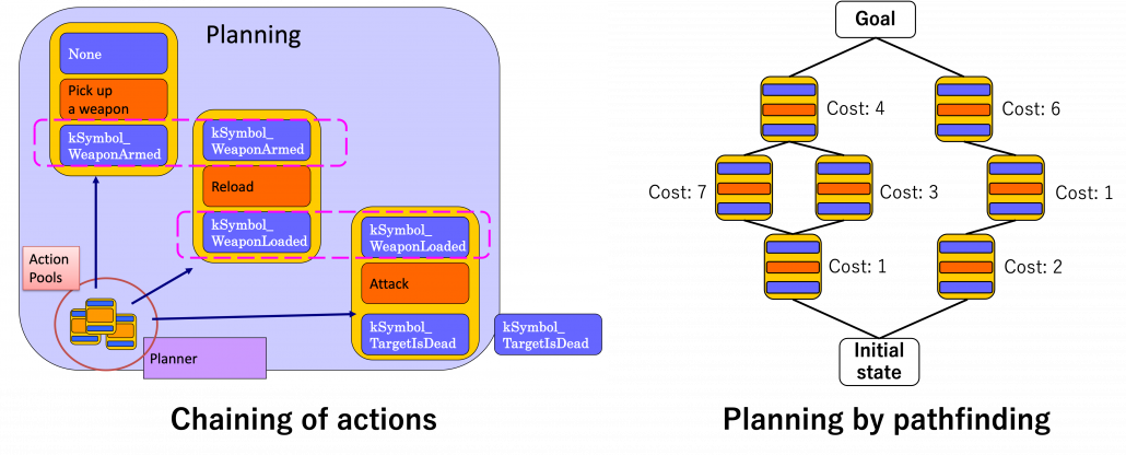
But with more options of actions like most of video games, forward plannings have to deal much larger sizes of future action combinations. GOAP enables realistic behaviors of character AI with a heuristic idea of planning backward. To borrow Miyake Youichiro’s expression, GOAP processes actions like sticky notes. On each sticky note, there is a combination of symbols like “whether a target is dead,” “whether a weapon is armed,” or “whether the weapon is loaded.” A sticky note composed of such symbols form an action, and each action comprises a prerequisite, an action, and an effect. And behaviors of character AI is conducted with planning like pasting the sticky notes.

More practically sticky notes, namely actions are stored in actions pools. For a decision making, as displayed in the left side of the figure below, actions are connected as a chain. First an action of a goal is first set, and an action can be connected to the prerequisite of the goal via its effect. Just as well corresponding former actions are selected until the initial state.  In the example of chaining below, the goal is “kSymbol_TargetIsDead,” and actions are chained via “kSymbol_TargetIsDead,” “kSymbol_WeaponLoaded,” “kSymbol_WeaponArmed,” and “None.” And there are several combinations of actions to reach a certain goal, so more practically each action has a cost, and the most ideal behavior of character AI is chosen by pathfinding on a graph like the right side of the figure below. And the best planning is chosen by a pathfinding algorithm.
Even though many of highly intelligent behaviors of character AI are implemented as backward plannings as I explained, planning forward can be very effective in some situations. Board game AI is a good example. A searching algorithm named Monte Carlo tree search is said to be one breakthroughs in board game AI. The searching algorithm randomly plays a game until the end, which is called playout. Numerous times of playouts enables evaluations of possibilities of winning. Monte Carlo Tree search also enables more efficient searches of games trees.

Meta AI

Meta AI is a type of AI such that controls a whole video game to enhance player’s experiences. To be more concrete, it adjusts difficulties of video games by for example dynamically arranging enemies. I think differences between meta AI and navigation AI or character AI can be also ambiguous. As I explained, the earliest video games were composed mainly with navigation AI, or rather just objects. Even if there are aliens or monsters, they can be just part of interactive objects as long as they move deterministically. I said character AI gave some diversities to their behaviors, but how challenging a video game is depends on dynamic arrangements of such objects or enemies. And some of classical video games like “Xevious,” as a matter of fact implemented such adjustments of difficulties of game plays. That is an advent of meta AI, but I think they were not so much distinguished from other types of AI, and I guess meta AI has been unconsciously just a part of programming.

It is said a turning point of modern meta AI is a shooting game “Left 4 Dead” released in 2008, where zombies are dynamically arranged. As well as many masterpiece thriller films, realistic and tense terrors are made by combinations of intensities and relaxations. Tons of monsters or zombies coming up one after another and just shooting them look stupid or almost like comedies. .And analyzing the success of “Counter-Strike,” they realized that users liked rhythms of intensity and relaxation, so they implemented that explicitly in “Left 4 Dead.” The graphs below concisely shows how meta AI works in the video game. When the survivor intensity, namely players’ intensity is low, the meta AI arrange some enemies. Survivor intensity increases as players fight with zombies or something, and then meta AI places fewer enemies so that players can relax. While players re relatively relaxing, desired population of enemies increases when they actually show up in video games, again the phase of intensity comes.

*Soul series video games do not seem to use meta AI so much. Characters in the games are rearranged in more or less the same ways every time players fail. Soul-like games make much of experiences that players find solutions by themselves, which means that manual but very careful arrangements of enemies and interactive objects are also very effective.

Meta AI can be used to make video games more addictive using data analysis. Recent social network games can record logs of game plays. Therefore if you can observe a trend that more users unsubscribe when they get less rewards in certain online events, operating companies of the game can adjust chances of getting “rare” items.

Procedural AI and AI outside video games

How clearly you can have an image of what I am going to explain in this subsection would depend how recently you have played video games. If your memories of playing video games stops with good old days of playing side-scrolling ones like Super Mario Brothers, you should at first look up some videos of playing open world games. Open world means a use of a virtual reality in which players can move an behave with a high degree of freedom. The term open world is often used as opposed to the linear games, where players have process games in the order they are given. Once you are immersed in photorealistic computer graphic worlds in such open world games, you would soon understand why metaverse is attracting attentions these days. Open world games for example like “Fallout 4” are astonishing in that you can even talk to almost everyone in them. Just as “Elden Ring” changed former soul series video games into an open world one, it seems providing open world games is one way to keep competitive in the video game industry. And such massive world can be made also with a help of procedural AI. Procedural AI can be seen as a part of meta AI, and it generates components of games such as buildings, roads, plants, and even stories. Thanks to procedural AI, video game companies with relatively small domestic markets like Poland can make a top-level open world game such as “The Witcher 3: Wild Hunt.”

An example of technique of procedural AI adopted in “The Witcher 3: Wild Hunt” for automatically creating the massive open world.

Creating a massive world also means needs of tons of debugging and quality assurance (QA). Combining works by programmers, designers, and procedural AI will cause a lot of unexpected troubles when it is actually played. AI outside game can be used to find these problems for quality assurance. Debugging and and QA have been basically done manually, and especially when it comes to QA, video game manufacturer have to employ a lot of gamer to let them just play prototype of their products. However as video games get bigger and bigger, their products are not something that can be maintained manually anymore. If you have played even one open world game, that would be easy to imagine, so automatic QA would remain indispensable in the video game industry. For example an open world game “Horizon Zero Dawn” is a video game where a player can very freely move around a massive world like a jungle. The QA team of this video game prepared bug maps so that they can visualize errors in video games. And they also adopted a system named “Apollo-Autonomous Automated Autobots” to let game AI automatically play the video game and record bugs.
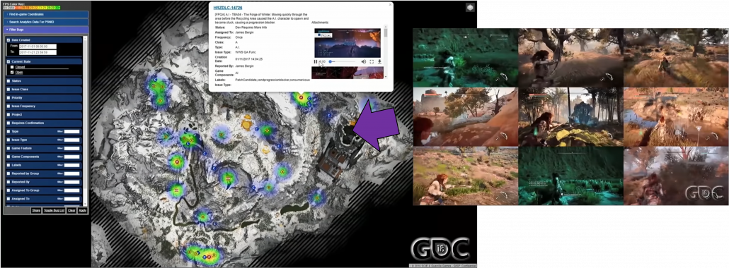
As most video games both in consoles or PCs are connected to the internet these days, these bugs can be fixed soon with updates. In addition, logs of data of how players played video games or how they failed can be stored to adjust difficulties of video games or train game AI. As you can see, video games are not something manufacturers just release. They are now something develop interactively between users and developers, and players’ data is all exploited just as your browsing history on the Internet.

I have briefly explained AI used for video games over four topics. In the next two sections, I am going to explain how board games and video games can be used for AI research.

3, Reinforcement learning: we might be a sort of well-made game AI models

Machine learning, especially RL is replacing humans with computers, however with incredible computation resources. Invention of game AI, in this context including computers playing board games, has been milestones of development of AI for decades. As Western countries had been leading researches on AI, defeating humans in chess, a symbol of intelligence, had been one of goals. Even Alan Turing, one of the fathers of computers, programmed game AI to play chess with one of the earliest calculators. Searching algorithms with game trees were mainly studied in the beginning. Game trees are a type of tree graphs to show how games proceed, by expressing future possibilities with diverging tree structures. And searching algorithms are often used on tree graphs to ignore future steps which are not likely to be effective, which often looks like cutting off branches of trees. As a matter of fact, chess was so “simple” that searching algorithms alone were enough to defeat Garry Kasparov, the world chess champion at that time in 1997. That is, growing trees and trimming them was enough for the “simplicity” of chess as long as a super computer of IBM was available. After that computer defeated one of the top players of shogi, a Japanese version of chess, in 2013. And remarkably, in 2016 AlphaGo of DeepMind under Google defeated the world go champion. Game AI has been gradually mastering board games in order of increasing search space size.

We can say combinations of techniques which developed in different streams converged into game AI today, like I display in the figure below. In AlphaGo or maybe also general game AI, neural networks enable “intuition” on phases of board games, searching algorithms enables “foreseeing,” and RL “experiences.” And as almost no one can defeat computers in board games anymore, the next step of game AI is how to conquer other video games.  Since progress of convolutional neural network (CNN) in this 3rd AI boom, computers got “eyes” like we do, and the invention of ResNet in 2015 is remarkable. Thus we can now use displays of video games as inputs to neural networks. And combinations of reinforcement learning and neural networks like (CNN) is called deep reinforcement learning. Since the advent of deep reinforcement learning, many people are trying to apply it on various video games, and they show impressive results. But in general that is successful in bird’s-eye view games. Even if some of researches can be competitive or outperform human players, even in first person shooting video games, they require too much computational resources and heuristic techniques. And usually they take too much time and computer resource to achieve the level.

*Even though CNN is mainly used as “eyes” of computers, it is also used to process a phase of a board game. That means each phase of is processed like an arrangement of pixels of an image. This is what I mean by “intuition” of deep learning. Just as neural networks can recognize objects, depending on training methods they can recognize boards at a high level.

Now I would like you to think about what “smartness” means. Competency in board games tend to have correlations with mathematical skills. And actually in many cases people proficient in mathematics are also competent in board games. Even though AI can defeat incredibly smart top board game players to the best of my knowledge game AI has yet to play complicated video games with more realistic computer graphics. As I explained, behaviors of character AI is in practice implemented as simpler graphs, and tactics taken in such graphs will not be as complicated as game trees of competitive board games. And the idea of game AI playing video games itself not new, and it is also used in debugging of video games. Thus the difficulties of computers playing video games would come more from how to associate what they see on displays with more long-term and more abstract plannings. And currently, kids would more flexibly switch to other video games and play them more professionally in no time. I would say the difference is due to frames of tasks. A frame roughly means a domain or a range which is related to a task. When you play a board game, its frame is relatively small because everything you can do is limited in the rule of the game which can be expressed as simple data structure. But playing video games has a wider frame in that you have to recognize only the necessary parts important for playing video games from its constantly changing displays, namely sequences of RGB images. And in the real world, even a trivial action like putting a class on a table is selected from countless frames like what your room looks like, how soft the floor is, or what the temperature is. Human brains are great in that they can pick up only necessary frames instantly.

As many researchers would already realize, making smaller models with lower resources which can learn more variety of tasks is going to be needed, and it is a main topic these days not only in RL but also in other machine learning. And to be honest, I am skeptical about industrial or academic benefits of inventing specialized AI models for beating human players with gigantic computation resources. That would be sensational and might be effective for gathering attentions and funds. But as many AI researchers would already realize, inventing a more general intelligence which would more flexibly adjust to various tasks is more important. Among various topics of researches on the problem, I am going to pick up transfer learning in the next section, but in a more futuristic and dreamy sense.

4, Transfer learning and game for AI

In an event with some young shogi players, to a question “What would you like to request to a god?” Fujii Sota, the youngest top shogi player ever, answered “If he exists, I would like to ask him to play a game with me.” People there were stunned by the answer. The young genius, contrary to his sleepy face, has an ambition which only the most intrepid figures in mythology would have had. But instead of playing with gods, he is training himself with game AI of shogi. His hobby is assembling computers with high end CPUs, whose performance is monstrous for personal home uses. But in my opinion such situation comes from a fact that humans are already a kind of well-made machine learning models and that highly intelligent games for humans have very limited frames for computers.

*It seems it is not only computers that need huge energy consumption to play board games. Japanese media often show how gorgeous and high caloric shogi players’ meals are during breaks. And more often than not, how fancy their feasts are is the only thing most normal spectators like me in front of TVs can understand, albeit highly intellectual tactics made beneath the wooden boards.

As I have explained, the video game industry has been providing complicated simulational worlds with sophisticated ensemble of game AI in both symbolism and connectionism ways. And such simulations, initially invented to hunt down players, are these days being conquered especially by RL models, and the trend showed conspicuous progress after the advent of deep learning, that is after computers getting “eyes.” The next problem is how to transfer the intelligence or experiences cultivated in such simulations to the real world. Only humans can successfully train themselves with computer simulations today as far as I know, but more practically it is desired to transfer experiences with wider frames to more inflexible entities like robots. Such technologies would be ideal especially for RL because physical devices cannot make numerous trial and errors in the real world. They should be trained in advance in computer simulations. And transfer learning could be one way to take advantages of experiences in computer simulations to the real world. But before talking about such transfer learning, we need to be careful about the term “transfer learning.” Transfer learning is a family of machine learning technologies to makes uses of knowledge learned in a dataset, which is usually relatively huge, to another task with another dataset. Even though I have been emphasizing transferring experiences in computer simulations, transfer learning is a more general idea applicable to more general use cases, also outside computer simulations. Or rather, transfer learning is attracting a lot of attentions as a promising technique for tackling lack of data in general machine learning. And another problem is even though transfer learning has been rapidly developing recently, various research topics are scattered in the field called “transfer learning.” And arranging these topics would need extra articles or something. Thus in the rest of this article,  I would like to especially focus on uses of video games or computer simulations in transfer learning. When it comes to already popular and practical transfer learning techniques like fine tuning with pre-trained backbone CNN or BERT, I am planning to cover them with more practical introduction in one of my upcoming articles. Thus in this article, after simply introducing ideas of domains and transfer learning, I am going to briefly introduce transfer learning and explain domain adaptation/randomization.

Domain and transfer learning

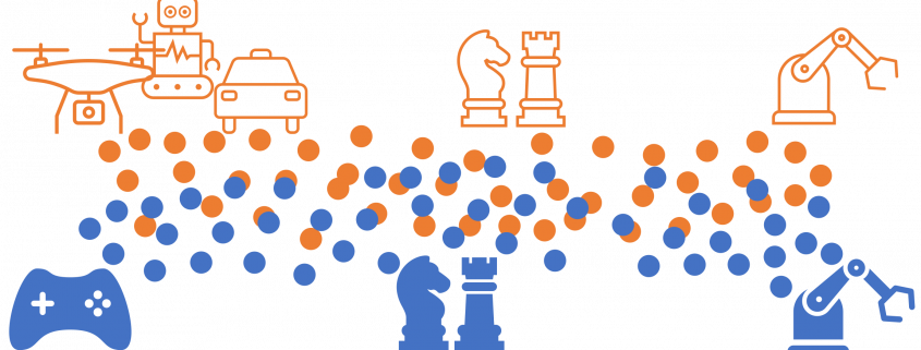
There is a more strict definition of a domain in machine learning, but all you have to know is it means in short a type of dataset used for a machine learning task. And different domains have a domain shift, which in short means differences in the domains. A text dataset and an image dataset have a domain shift. An image dataset of real objects and one with cartoon images also have a smaller domain shift. Even differences in lighting or angles of cameras would cause a domain  shift. In general, even if a machine learning model is successful in tasks in a domain, even a domain shift which is trivial to humans declines performances of the model. In other words, intelligence learned in one domain is not straightforwardly applicable to another domain as humans can do. That is, even if you can recognize objects both a real and cartoon cars as a car, that is not necessarily true of machine learning models. As a family of techniques for tackling this problem, transfer learning makes a use of knowledge in a source domain (the dots in blue below), and apply the knowledge to a target domain. And usually, a source domain is assumed to be large and labeled, and on the other hand a target domain is assumed to be relatively small or even unlabeled. And tasks in a source or a target domain can be different. For example, CNN models trained on classification of ImageNet can be effectively used for object detection. Or BERT is trained on a huge corpus in a self-supervised way, but it is applicable to a variety of tasks in natural language processing (NLP).

*To people in computer vision fields, an explanation that BERT is a NLP version of pre-trained CNN would make the most sense. Just as a pre-trained CNN maps an image, arrangements of RGB pixels values, to a vector representing more of “meaning” of the image, BERT maps a text,  a sequence of one-hot encodings, into a vector or a sequence of vectors in a semantic field useful for NLP.

Transfer learning is a very popular topic, and it is hard to arrange and explain types of existing techniques. I think that is because many people are tackling more or less the similar problems with slightly different approaches. For now I would like you to keep it in mind that there are roughly three points below to consider in transfer learning

  1. What to transfer
  2. When to transfer
  3. How to transfer

The answer of the second point above “When to transfer” is simply “when domains are more or less alike.” Transfer learning assume similarities between target and source domains to some extent. “How to transfer” is very task-specific, so this is not something I can explain briefly here. I think the first point “what to transfer” is the most important for now to avoid confusions about what “transfer learning” means. “What to transfer” in transfer learning is also classified to the three types below.

  • Instance transfer (transferring datasets themselves)
  • Feature transfer (transferring extracted features)
  • Parameter transfer (transferring pre-trained models)

In fact, when you talk about already practical transfer learning techniques like using pre-trained CNN or BERT, they refer to only parameter transfer above. And please let me skip introducing it in this article. I am going to focus only on techniques related to video games in this article.

*I would like to give more practical introduction on for example BERT in one of my upcoming articles.

Domain adaptation or randomization

I first got interested in relations of video games and AI research because I was studying domain adaptation, which tackles declines of machine learning performance caused by a domain shift. Domain adaptation is sometimes used as a synonym to transfer learning. But compared to that general transfer learning also assume different tasks in different domains, domain adaptation assume the same task. Thus I would say domain adaptation is a subfield of transfer learning. There are several techniques for domain adaptation, and in this article I would like to take feature alignment as an example of frequently used approaches. Input datasets have a certain domain shift like blue and circle dots in the figure below. This domain shift cannot be changed if datasets themselves are not directly converted. Feature alignment make the domain shift smaller in a feature space after data being processed by the feature extractor. The features expressed as square dots in the figure are passed to task-specific networks just as normal machine learning. With sufficient labels in the source domain and with fewer or no labels in the target one, the task-specific networks are supervised. On the other hand, the features are also passed to the domain discriminator, and the discriminator predicts which domain the feature comes from. The domain discriminator is normally trained with supervision by classification loss, but the feature supervision is reversed when it trains the feature extractor. Due to the reversed supervision the feature extractor learns mix up features because that is worse for discriminating distinguishing the source or target domains. In this way, the feature extractor learns extract domain invariant features, that is more general features both domains have in common.

*The feature extractor and the domain discriminator is in a sense composing generative adversarial networks (GAN), which is often used in data generation. To know more about GAN, you could check for example this article.

One of motivations behind domain adaptation is that it enables training AI tasks with synthetic datasets made by for example computer graphics because they are very easy to annotate and prepare labels necessary for machine learning tasks. In such cases, domain invariant features like curves or silhouettes are expected to learn. And learning computer vision tasks from GTA5 dataset which are applicable to Cityscapes dataset is counted as one of challenging tasks in papers on domain adaptation. GTA of course stands for “Grand Theft Auto,” the video open-world video game series. If this research continues successfully developing, that would imply possibilities of capability of teaching AI models to “see” only with video games. Imagine that a baby first learns to play Grand Theft Auto 5 above all and learns what cars, roads, and pedestrians are.  And when you bring the baby outside, even they have not seen any real cars, they point to a real cars and people and say “car” and “pedestrians,” rather than “mama” or “dada.”

In order to enable more effective domain adaptation, Cycle GAN is often used. Cycle GAN is a technique to map texture in one domain to another domain. The figure below is an example of applying Cycle GAN on GTA5 dataset and Cityspaces Dataset, and by doing so shiny views from a car in Los Santos can be converted to dark and depressing scenes in Germany in winter. This instance transfer is often used in researches on domain adaptation.
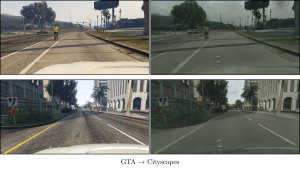
Even if you mainly train depth estimation with data converted like above, the model can predict depth data of the real world domain without correct depth data. In the figure below, A is the target real data, B is the target domain converted like a source domain, and C is depth estimation on A.
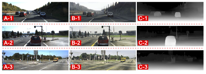
Crowd counting is another field where making a labeled dataset with video games is very effective. A MOD for making a crowd arbitrarily is released, and you can make labeled datasets like below.

*Introducing GTA mod into research is hilarious. You first need to buy PC software of Grand Theft Auto 5 and gaming PC at first. And after finishing the first tutorial in the video game, you need to find a place to place a camera, which looks nothing but just playing video games with public money.

Domain adaptation problems I mentioned are more of matters of how to let computers “see” the world with computer simulations. But the gap between the simulational worlds and the real world does not exist only in visual ways like in CV. How robots or vehicles are parametrized in computers also have some gaps from the real world, so even if you replace only observations with simulations, it would be hard to train AI. But surprisingly, some researches have already succeeded in training robot arms only with computer simulations. An approach named domain randomization seems to be more or less successful in training robot arms only with computer simulations and apply the learned experience to the real world. Compared to domain adaptation aligned source domain to the target domain, domain randomization is more of expanding the source domain by changing various parameters of the source domain. And the target domain, namely robot arms in the real world is in the end included in the expanded source domain. And such expansions are relatively easy with computer simulations.

For example a paper “Closing the Sim-to-Real Loop: Adapting Simulation Randomization with Real World Experience” proposes a technique to reflect real world feed back to simulations in domain randomization, and this pipeline enables a robot arm to do real world tasks in a few iteration of real world trainings.

As the video shows, the ideas of training a robot with computer simulations is becoming more realistic.

The future of games for AI

I have been emphasizing how useful video games are in AI researches, but I am not sure if how much the field purely rely on video games like it is doing especially on RL. Autonomous driving is a huge research field, and modern video games like Grand Thef Auto are already good driving simulations in urban areas. But other realistic simulations like CARLA have been developed independent of video games. And in a paper “Exploring the Limitations of Behavior Cloning for Autonomous Driving,” some limitations of training self-driving cars in the simulation are reported. And some companies like Waymo switched to recurrent neural networks (RNN) for self-driving cars. It is natural that fields like self-driving, where errors of controls can be fatal, are not so optimistic about adopting RL for now.

But at the same time, Microsoft bought a Project Bonsai, which is aiming at applying RL to real world tasks. Also Microsoft has Project Malmo or AirSim, which respectively use Minecraft or Unreal Engine for AI reseraches. Also recently the news that Microsoft bought Activision Blizzard was a sensation last year, and media’s interests were mainly about metaverse or subscription service of video games. But Microsoft also bouth Zenimax Media, is famous for open world like Fallout or Skyrim series. Given that these are under Microsoft, it seems the company has been keen on merging AI reserach and developing video games.

As I briefly explained, video games can be expanded with procedural AI technologies. In the future AI might be trained in video game worlds, which are augmented with another form of AI. Combinations of transfer learning and game AI might possibly be a family of self-supervising technologies, like an octopus growing by eating its own feet. At least the biggest advantage of the video game industry is, even technologies themselves do not make immediate profits, researches on them are fueled by increasing video game fans all over the world. This is a kind of my sci-fi imagination of the world. Though I am not sure which is more efficient to manually design controls of robots or training AI in such indirect ways. And I prefer to enhance physical world to metaverse. People should learn to put their controllers someday and to enhance the real world. Highly motivated by “Elden Ring” I wrote this article. Some readers might got interested in the idea of transferring experiences in computer simulations to the real world. I am also going to write about transfer learning in general that is helpful in practice.

* I make study materials on machine learning, sponsored by DATANOMIQ. I do my best to make my content as straightforward but as precise as possible. I include all of my reference sources. If you notice any mistakes in my materials, including grammatical errors, please let me know (email: yasuto.tamura@datanomiq.de). And if you have any advice for making my materials more understandable to learners, I would appreciate hearing it.
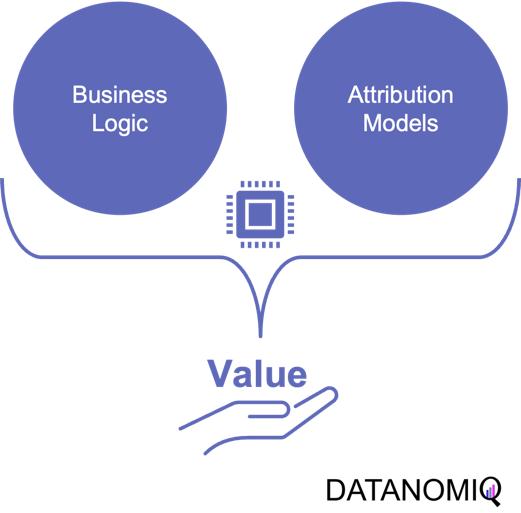
AI Role Analysis in Cybersecurity Sector

Cybersecurity as the name suggests is the process of safeguarding networks and programs from digital attacks. In today’s times, the world sustains on internet-connected systems that carry humungous data that is highly sensitive. Cyberthreats are on the rise with unscrupulous hackers taking over the entire industry by storm, with their unethical practices. This not only calls for more intense cyber security laws, but also the vigilance policies of the corporates, big and small, government as well as non-government; needs to be revisited.

With such huge responsibility being leveraged over the cyber-industry, more and more cyber-security enthusiasts are showing keen interest in the industry and its practices. In order to further the process of secured internet systems for all, unlike data sciences and other industries; the Cybersecurity industry has seen a workforce rattling its grey muscle with every surge they experience in cyber threats. Talking of AI impressions in Cybersecurity is still in its nascent stages of deployment as humans are capable of more; when assisted with the right set of tools.

Automatically detecting unknown workstations, servers, code repositories, and other hardware and software on the network are some of the tasks that could be easily managed by AI professionals, which were conducted manually by Cybersecurity folks. This leaves room for cybersecurity officials to focus on more urgent and critical tasks that need their urgent attention. Artificial intelligence can definitely do the leg work of processing and analyzing data in order to help inform human decision-making.

AI in cyber security is a powerful security tool for businesses. It is rapidly gaining its due share of trust among businesses for scaling cybersecurity. Statista, in a recent post, listed that in 2019, approximately 83% of organizations based in the US consider that without AI, their organization fails to deal with cyberattacks. AI-cyber security solutions can react faster to cyber security threats with more accuracy than any human. It can also free up cyber security professionals to focus on more critical tasks in the organization.

CHALLENGES FACED BY AI IN CYBER SECURITY

As it is said, “It takes a thief to catch a thief”. Being in its experimental stages, its cost could be an uninviting factor for many businesses. To counter the threats posed by cybercriminals, organizations ought to level up their internet security battle. Attacks backed by the organized crime syndicate with intentions to dismantle the online operations and damage the economy are the major threats this industry face today. AI is still mostly experimental and, in its infancy, hackers will find it much easy to carry out speedier, more advanced attacks. New-age automation-driven practices are sure to safeguard the crumbling internet security scenarios.

AI IN CYBER SECURITY AS A BOON

There are several advantageous reasons to embrace AI in cybersecurity. Some notable pros are listed below:

  •  Ability to process large volumes of data
    AI automates the creation of ML algorithms that can detect a wide range of cybersecurity threats emerging from spam emails, malicious websites, or shared files.
  • Greater adaptability
    Artificial intelligence is easily adaptable to contemporary IT trends with the ever-changing dynamics of the data available to businesses across sectors.
  • Early detection of novel cybersecurity risks
    AI-powered cybersecurity solutions can eliminate or mitigate the advanced hacking techniques to more extraordinary lengths.
  • Offers complete, real-time cybersecurity solutions
    Due to AI’s adaptive quality, artificial intelligence-driven cyber solutions can help businesses eliminate the added expenses of IT security professionals.
  • Wards off spam, phishing, and redundant computing procedures
    AI easily identifies suspicious and malicious emails to alert and protect your enterprise.

AI IN CYBERSECURITY AS A BANE

Alongside the advantages listed above, AI-powered cybersecurity solutions present a few drawbacks and challenges, such as:

  • AI benefits hackers
    Hackers can easily sneak into the data networks that are rendered vulnerable to exploitation.
  • Breach of privacy
    Stealing log-in details of the users and using them to commit cybercrimes, are deemed sensitive issues to the privacy of an entire organization.
  • Higher cost for talents
    The cost of creating an efficient talent pool is very high as AI-based technologies are in the nascent stage.
  • More data, more problems
    Entrusting our sensitive data to a third-party enterprise may lead to privacy violations.

AI-HUMAN MERGER IS THE SOLUTION

AI professionals backed with the best AI certifications in the world assist corporations of all sizes to leverage the maximum benefits of the AI skills that they bring along, for the larger benefit of the organization. Cybersecurity teams and AI systems cannot work in isolation. This communion is a huge step forward to leveraging maximum benefits for secured cybersecurity applications for organizations. Hence, this makes AI in cybersecurity a much-coveted aspect to render its offerings in the long run.

Stop saying “trial and errors” for now: seeing reinforcement learning through some spectrums

*This is the fourth article of the series My elaborate study notes on reinforcement learning.

*In this article series “the book by Barto and Sutton” means “Reinforcement Learning: An Introduction second edition.” This book is said to be almost mandatory for those who seriously learn Reinforcement Learning (RL). And “the whale book” means a Japanese textbook named 「強化学習 (機械学習プロフェッショナルシリーズ)」(“Reinforcement Learning (Machine Learning Processional Series)”), by Morimura Tetsuro. I would say the former is for those who want to mainly learn how to use RL, and the latter is for more theoretical understanding. I am trying to make something between them in my series.

1, Finally to reinforcement learning

Some of you might have got away with explaining reinforcement learning (RL) only by saying an obscure thing like “RL enables computers to learn through trial and errors.” But if you have patiently read my articles so far, you might have come to say “RL is a family of algorithms which simulate procedures similar to dynamic programming (DP).” Even though my article series has not covered anything concrete and unique to RL yet, I think my series has already laid a hopefully effective foundation of discussions on RL. And in the first article, I already explained that “trial and errors” are only agents’ actions for collecting data from the environment. Such “trial and errors” lead to “experiences” of computers. And in this article we can finally start discussing how computers “experience” things in more practical and theoretical ways.

*The expression “to learn” is also frequently used in contexts of other machine learning algorithms. Thus in order to clearly separate the ideas, let me use the expression “to experience” when it comes to explaining RL. At any rate, what computers are doing is updating parameters, and in RL also updating values and policies. But some terms related to RL also use the word “experience,” for example experience replay, so “to experience” might be a preferred phrase in RL fields.

I think changing discussions on DP into those on RL is like making graphs more “open” rather than “closed.” In the second article, I explained DP problems, where the models of environments are completely known, as repeatedly updating graphs like neural networks. As I have been repeatedly saying RL, or at least model-free RL, is an approximated application of DP in the environments without a complete model. That means, connections of nodes of the graph, that is relations of actions and states, are something agents have to estimate directly or indirectly. I think that can be seen as untying connections of the graphs which I displayed when I explained DP. By doing so, I propose to see RL or more exactly model-free RL like the graph of the right side of the figure below.

*For the time being, I would prefer to use the term model-free RL rather than just RL. That is not only because this article is about model-free RL but also because I want to avoid saying inaccurate things about wider range of RL algorithms I would have to study more precisely and explain.

Some people might say these are tree structures, and that might be technically correct. But in my sense, this is more of “willows.” The cover of the second edition of the books by Barto and Sutton also looks like willows. The cover design comes from a paper on RL named “Learning to Drive a Bicycle using Reinforcement Learning and Shaping.” The paper is about learning to ride a bike in a simulator with RL. The geometric patterns are not models of human brain nerves, but trajectories of an agent learning to balance a bike. However interestingly, the trajectories of the bike, which are inscribed on a road, partly diverge but converge in a certain way as a whole, like the RL graph I propose. That is why I chose some pictures of 「花札 (hanafuda)」as the main picture of this series. Hanafuda is a Japanese gamble card game with monthly seasonal flower pictures. And the cards of June have pictures of willows.

Source: Learning to Drive a Bicycle using Reinforcement Learning and Shaping, Randløv, (1998)    Richard S. Sutton, Andrew G. Barto, “Reinforcement Learning: An Introduction,” MIT Press, (2018)

2, Untying DP graphs: planning or learning

Even though I have just loudly declared that my RL graphs are more of “willow” structures in my aesthetic sense, I must admit they should basically be discussed as popular tree structures. That is because, when you start discussing practical RL algorithms you need to see relations of states and actions as tree structures extending. If you already more or less familiar with tree structures or searching algorithms on tree graphs, learning RL with tree structures should be more or less straightforward to you. Another reason for using tree structures with nodes of states and actions is that the book by Barto and Sutton use buck up diagrams of Bellman equations which are tree graphs. But I personally think the graphs should be used more effectively, so I am trying to expand its uses to DP and RL algorithms in general. In order to avoid confusions about current discussions on RL in my article series, I would like to give an overall review on how to look at my graphs.

The graphs in the figure below are going to be used in my articles, at least when I talk about model-free RL. I made them based on the backup diagram of Bellman equation introduced in the book by Barto and Sutton. I would like you to first remember that in RL we are basically discussing Markov decision process (MDP) environment, where the next action and the resulting next states depends only on the current state. Such models are composed of white nodes representing each state s in an state space \mathcal{S}, and black nodes representing each action a, which is a member of an action space \mathcal{A}. Any behaviors of agents are represented as going back and forth between black and white nodes of the model, and that is why connections in the MDP model are bidirectional.  In my articles let me call such model of environments “a closed model.” RL or general planning problems are matters of optimizing policies in such models of environments. Optimizing the policies are roughly classified into two types, planning/searching or RL, and the main difference between them is whether connections of graphs of models are known or not. Planning or searching is conducted without actually moving in the environment. DP are family of planning algorithms which are known to converge, and so far in my articles we have seen that DP are enabled by repeatedly applying Bellman operators. But instead of considering and updating all the possible transitions in the model like DP, planning can be conducted more sparsely. Such sparse planning are often called searching, and many of them use tree structures. If you have learned any general decision making problems with tree graphs, you might be already familiar with some searching techniques like alpha-beta pruning.

*In explanations on DP in my articles, directions of connections of model graphs are confusing, so I precisely explained how to look at them in the second section in the last article.

On the other hand, RL algorithms are matters of learning the linkages of models of environments by actually moving in them. For example, when the agent in the figure below move on a grid map like the purple arrows, the movement is represented like in the closed model in the middle. However as the agent does not have the complete closed model, the agent has to move around in the environment like the tree structure at the right side to learn values of each node.

The point is, whether models of environments are known or unknown, or whether agents actually move in the environment or not, movements of agents are basically represented as going back and forth between white nodes and black nodes in closed models. And such closed models are entangled in searching or RL. They are similar operations, but they are essentially different in that searching agents do not actually move in searching but in RL they actually move.  In order to distinguish searching and learning, in my articles, trees for searching are extended vertically, trees for learning horizontally.

*DP and searching are both planning, but DP consider all the connections of actions and states by repeatedly applying Bellman operators. Thus I would not count DP as “untying” of closed models.

3, Some spectrums in RL algorithms

Starting studying actual RL algorithms also means encountering various algorithms one after another. Some of you might have already been overwhelmed by new terms coming up one after another in study materials on RL. That is because, as I explained in the first article, RL is more about how to train models of values or policies. Thus it is natural that compared to general machine learning, which more or less share the same training frameworks, RL has a variety of training procedures. Rather than independently studying each RL algorithm, I think it is more effective to see connections of each algorithm, which is linked by adjusting degrees of some important elements in RL. In fact I have already introduced those elements as some pairs of key words of RL in the first article. But it would be all the more effective to review them, especially after learning DP algorithms as representative planning methods. If you study RL that way, you would come to see trial and errors or RL as a crucial but just one aspect of RL.

I think if you care less about the trial-and-error aspect of RL that allows you to study RL more effectively in the beginning. And for the time being, you should stop viewing RL in the popular way as presented above. Not that I am encouraging you to ignore the trial and error part, namely relations of actions, rewards, and states. My point is that it is more of inside the agent that should be emphasized. Planning, including DP is conducted inside the agent, and trial and errors are collection of data from the environment for the sake of the planning. That is why in many study materials on RL, DP is first introduced. And if you see differences of RL algorithms as adjusting of some pairs of elements of planning problems, it would be less likely that you would get lost in curriculums on RL. The pairs are like some spectrums. Not that you always have to choose either of each pair, but rather ideal solutions are often in the middle of the two ends of the spectrums depending on tasks. Let’s take a look at the types of those spectrums one by one.

(1) Value-policy or actor-critic spectrum

The crucial type of spectrum you should be already familiar with is the value-policy one. I think this spectrum can be adjusted in various ways. For example, over the last two articles we have seen how values and policies reach the optimal functions in DP using policy iteration or value iteration. Policy iteration alternates between updating values and policies until convergence to the optimal policy, whereas value iteration keeps updating only values until reaching the optimal value, to get the optimal policy at the end. And similar discussions can be seen also in the upcoming RL algorithms. The book by Barto and Sutton sees such operations in general as generalized policy iteration (GPI).

Source: Richard S. Sutton, Andrew G. Barto, “Reinforcement Learning: An Introduction,” MIT Press, (2018)

You should pay attention to the idea of GPI because this is what makes RL different form other general machine learning. In many cases RL is explained as a field of machine learning which is like trial and errors, but I personally think that GPI, interactive optimization between values and policies, should be more emphasized. As I said in the first article, RL optimizes decision making rules, that is policies \pi(a|s), in MDPs. Other general machine learning algorithms have more direct supervision by loss functions and models are optimized so that loss functions are minimized. In the case of the figure below, an ML model f is optimized to f_{\ast} by optimization such as gradient descent. But on the other hand in RL policies \pi do not have direct loss functions. Then RL uses values v(s), which are functions of how good it is to be in states s. As one part of GPI, the value function v_{\pi} for the current policy \pi is calculated, and this is called estimation in the book by Barto and Sutton.  And based on the estimated value function, the policy is improved as \pi ', which is called policy improvement, and overall processes of estimation and policy improvement are called control in the book. And v_{\pi} and \pi are updated alternately this way until converging to the optimal values v_{\ast} or policies \pi_{\ast}. This interactive updates of values and policies are done inside the agent, in the dotted frame in red below. I personally think this part should be more emphasized than trial-and-error-like behaviors of agents. Once you see trial and errors of RL as crucial but just one aspect of GPI and focus more inside agents, you would see why so many study materials start explaining RL with DP.

You can explicitly model such interactions of values and policies by modeling each of them with different functions, and in this case such frameworks of RL in general are called actor-critic methods. I am gong to explain actor-critic methods in an upcoming article. Thus the value-policy spectrum also can be seen as a actor-critic spectrum. Differences between the pairs of value-policy or actor-critic spectrums are something you would little by little understand. For now I would say GPI is the most general and important idea behind RL. But practical RL algorithms are implemented as actor-critic methods. Critic parts gives some signals to actor parts, and critic parts get its consequence by actor parts taking actions in environments. Not that actors directly give feedback to critics.

*I think one of confusions in studying RL come from introducing Q-learning or SARSA at the first algorithms or a control in RL. As I have said earlier, interactive relations between values and policies or actors and critics, that is GPI, should be emphasized. And I think that is why DP is first introduced in many books. But in Q-learning or SARSA, an actor and a critic parts are combined as one module. But explicitly separating the actor and critic parts would be just too difficult at the beginning. And modeling an actor and a critic with separate modules would lead to difficulties in optimizing them together.

(2) Exploration-exploitation or on-off policy spectrum

I think the most straightforward spectrum is the exploitation-exploration spectrum. You can adjust how likely agents take random actions to collect data. Occasionally it is ideal for agents to have some degree of randomness in taking actions to explore unknown states of environments. One of the simplest algorithms to formulate randomness of actions is ε-greedy method, which I explained in the first article. In this method in short agents take a random action with a probability of ε. Instead of arbitrarily setting a hyperparameter \epsilon, randomness of actions can be also learned by modeling policies with certain functions. This randomness of functions can be also modeled in actor-critic frameworks. That means, depending on a choice of an actor, such actor can learn randomness of actions, that is explorations.

The two types of spectrums I have introduced so far lead to another type of spectrum. It is an on-off policy spectrum. Even though I explained types of policies in the last article using examples of home-lab-Starbucks diagrams, there is another way to classify policies: there are target policies and behavior policies. The former are the very policies whose optimization we have been discussing. The latter are policies for taking actions and collecting data. When agents use target policies also as behavior policies, they are on-policy algorithms. If agents use different policies for taking actions during optimization of target policies, they are off-policy methods.

Policy iteration and value iteration of DP can be also classified into on-policy or off-policy in a sense. In policy iteration values are updated using an up-to-date estimated policy, and the policy becomes optimal when it converges. Thus behavior and target policies are the same in this case. On the other hand in value iteration, values are updated with Bellman optimality operator, which updates values in a greedy way. Using greedy method means the policy \pi is not used for considering which action to take. Thus target and behavior policies are different. As you will see soon, concrete model-free RL algorithms like SARSA or Q-learning also have the same structure: the former is on-policy and the latter is off-policy. The difference of on-policy or off-policy would be more straightforward if we model behavior policies and target policies with different functions. An advantage of off-policy RL is you can model randomness of exploration of agents with extra functions. On the other hand, a disadvantage is that it would be harder to train different models at the same time. That might be a kind of tradeoff similar to an actor-critic method.

Even though this exploration-exploitation aspect of RL is relatively easy to understand, at the same time that can lead to much more complicated discussions on RL, which I would not be able to cover in this article series. I recommended you to stop seeing RL as trial and errors for the time being, but in the end trial and errors would prove to be crucial because data needed for GPI are collected mainly via trial and errors. Even if you implement some simple RL algorithms, you would soon realize it is hard to deal with unvisited states. Enough explorations need to be modeled by a behavior policy or some sophisticated heuristic techniques. I am planning to explain convergence of several RL algorithms, and they are guaranteed by sufficiently exploring all the states. However, thorough explorations of all the states lead to massive computational costs. But lack of exploration would let RL agents myopically overestimate current policies, never finding policies which pay off in the long run. That might be close to discussions on how to efficiently find a global minimum of a loss function, avoiding local minimums.

(3) TD-MonteCarlo spectrum

A variety of spectrums so far are enabled by modeling proper functions on demand. But in AI problems such functions are something which have to be automatically trained with some supervision. Instead of giving supervision explicitly with annotated data like in supervised learning of general machine learning, RL agents train models with “experiences.” As I am going to explain in the next part of this article, “experiences” in RL contexts mean making some estimations of values and adjusting such estimations based on actual rewards they get. And the timings of such feedback lead to another spectrum, which I call a TD-MonteCarlo spectrum. When the feedback happens every time an agent takes an action, it is TD method, on the other hand when that happens only at the end of an episode, that is Monte Carlo method. But it is easy to imagine that ideal solutions are usually at the middle of them. I am going to dig this topic soon in the next article. And n-step methods or TD(λ), which bridge the TD and Monte Carlo, are going to be covered in one of upcoming articles.

(4) Model free-based spectrum

The next spectrum might be relatively hard to understand, and to be honest I am still not completely sure about this topic. Please bear that in your mind. In the last section, I said RL is a kind of untying DP graphs and make them open because in RL, models of environments are unknown. However to be exact, that was mainly about model-free RL, which this article is going to cover for the time being. And I would say the graphs I showed in the last section were just two extremes of this model based-free spectrum. Some model-based RL methods exist in the middle of those two ends. In short RL agents can retain models of environments and do some plannings even when they do trial and errors. The figure below briefly compares planning, model-based RL, and model-free RL in the spectrum.

Let’s take a rough example of humans solving a huge maze. DP, which I have covered is like having a perfect map of the maze and making plans of how to move inside in advance. On the other hand, model-free reinforcement learning is like soon actually entering the maze without any plans. In model-free reinforcement learning, you only know how big the maze is, and you have a great memory for remembering in which directions to move, in all the places. However, as the model of how paths are connected is unknown, and you naively try to remember all the actions in all the places, it generally takes a longer time to solve the maze. As you could easily imagine, having some heuristic ideas about the model of the maze and taking some notes and making plans about courses would be the most efficient and the most peaceful. And such models in your head can be updated by actually moving in the maze.

*I believe that you would not say the pictures above are spoilers.

I need to more clearly talk about what a model is in RL or general planning problems. The book by Barto and Sutton simply defines a model this way: “By a model of the environment we mean anything that an agent can use to predict how the environment will respond to its actions. ” The book also says such models can be also classified to distribution models and sample models. The difference between them is the former describes an environment as combinations of known models, but the latter is like a black box model of an environment. An intuitive example is, as introduced in the book by Barto and Sutton, throwing dozens of dices can be seen in the both types. If you just throw the dices, sometimes chancing numbers of dices, and record the sum of the numbers on the dices s every time, that is equal to getting the sum from a black box. But a probabilistic distribution of such sums can be actually calculated as a multinomial distribution. Just as well, you can see a probability of transitions in an RL environment as a black box, but the probability can be also modeled. Some readers might have realized that distribution or sample models can be almost the same in the end, with sufficient data. In many cases of machine learning or statistics algorithms, complicated distributions have to be approximated with samples. Or rather how to approximate them is more of interest. In the case of dozens of dices, you can analytically calculate its distribution model as a multinomial distribution. But if you throw the dices numerous times, you would get precise approximated distributions.

When we discuss model-based RL, we need to consider not only DP but also other planning algorithms. DP is a family of planning algorithms which are known to converge, and many of RL algorithms share a lot with DP at theoretical levels. But in fact DP has one shortcoming even if the MDP model of an environment is known: DP needs to consider and update all the states. When models of environments are too complicated and large, applying DP is not a good idea. Also in many of such cases, you could not even get such a huge model of the environment. You would rather get only a black box model of the environment. Such a black box model only gets a pair of current state and action (s, a), and gives out the next state s' and corresponding reward r, that is the black box is a sample model. In this case other planning methods with some searching algorithms are used, for example Monte Carlo tree search. Such search algorithms are designed to more efficiently and sparsely search states and actions of interest. Many of searching algorithms used in RL make uses of tree structures. Model-based approaches can be roughly classified into three types below based on size or complication of models.

*As you could see, differences between sample models and distribution models can be very ambiguous. So are differences between model-free and model-based RL, I guess. As a matter of fact the whale book says the distributions of models approximated in model-free RL are the same as those in model-based ones. I cannot say anything exactly anymore, but I guess model-free RL is more of “memorizing” an environment, or combinations of states and actions in the environments. But memorizing environments can be computationally problematic in many cases, so assuming some distributions of models can help. That is my impression for now.

*Tree search algorithms alone shows very impressive performances, as long as you have massive computation resources. A heuristic tree search without reinforcement learning could defeat Garri Kasparow, a former chess champion, as long as enough computation resource is available. Searching algorithms were enough for “simplicity” of chess.

*I am not sure whether model-free RL algorithms are always simpler than model-based ones. For example Deep Q-Learning, a model-free method with some neural networks can learn to play Atari or Nintendo Entertainment System. Model-based deep RL is used in more complex task like AlphaGo or AlphaZero, which can defeat world champions of various board games. AlphaGo or AlphaZero models intuitions in phases of board games with convolutional neural networks (CNN), prediction of some phases ahead with search algorithms, and learning from past experiences with RL. I am not going to cover model-based RL in general in this series, but instead I would like to explain how RL enables computers to play video games after introducing some searching algorithms.

(5) Model expressivity spectrum

No matter how impressive or dreamy RL algorithms sound, their competence largely depend on model expressivity. In the first article, I emphasized “simplicity” of RL. DP or RL algorithms so far or in upcoming several articles consider incredibly simple cases like kids playbooks. And that beginning parts of most RL study materials cover only the left side of the figure below. In order to enable RL agents with more impressive tasks such as balancing cart-pole or playing video games, we need to raise the bar of expressivity spectrum, from the left to the right side of the figure below. You need to wait until a chapter or a section on “function approximation” in order to actually feel that your computer is doing trial and errors. And such chapters finally appear after reading half of both the book by Barto and Sutton and the whale book.

*And this spectrum is also a spectrum of computation costs or convergence. The left type could be easily implemented like programming assignments of schools since it in short needs only Excel sheets, and you would soon get results. The middle type would be more challenging, but that would not b computationally too expensive. But when it comes to the type at the right side, that is not something which should be done on your local computer. At least you need a GPU. You should expect some hours or days even for training RL agents to play 8 bit video games. That is of course due to cost of training deep neural networks (DNN), especially CNN. But another factors is potential inefficiency of RL. I hope I could explain those weak points of RL and remedies for them.

We need to model values and policies with certain functions. For the time being, in my articles values and policies are just modeled as tabular data, that is some NumPy arrays or Excel sheets. These are types of cases where environments and actions are relatively simple and discrete. Thus they can be modeled with some tabular data with the same degree of freedom. Assume a case where there are only 30 grids in an environment and only 4 types of actions in every grid. In such case, values are stored as arrays with 30 elements, and so are policies. But when environments are more complex or require continuous values of some parameters, values and policies have to be approximated with some models. When only relatively few parameters need to be estimated, simple machine learning models such as softmax functions can be used as such models. But compared to the cases with tabular data, convergence of training has to be discussed more carefully. And when you need to estimate continuous values, techniques like policy gradients have to be introduced. And we can dramatically enhance expressivity of models with deep neural netowrks (DNN), and such RL is called deep RL. Deep RL has showed great progress these days, and it is capable of impressive performances. Deep RL often needs observers to process inputs like video frames, and for example convolutional neural networks (CNN) can be used to make such observers. At any rate, no matter how much expressivity RL models have, they need to be supervised with some signals just as general machine learning often need labeled data. And “experiences” give such supervisions to RL agents.

(6) Adjusting sliders of spectrum

As you might have already noticed, these spectrums are not something you can adjust independently like faders on mixing board. They are more like some sliders for adjusting colors, brightness, or chroma on painting software. If you adjust one element, other parts are more or less influenced. And even though there are a variety of colors in the world, they continuously change by adjusting those elements of colors. Just as well, even if each RL algorithms look independent, many of them share more or less the same ideas, and only some parts are different in terms of their degrees. When you get lost in the course of studying RL, I would like you to decompose the current topic into these spectrums of RL elements I have explained.

I hope my explanations so far changed how you see RL. In the first article I already said RL is approximation of DP-like procedures with data collected by trial and errors, but from now on I would explain it also this way: RL is a family of algorithms which enable GPI by adjusting some spectrums.

In the next some articles, I am going to mainly cover RL algorithms named SARSA and Q-learning. Both of them use tabular data, and they are model-free. And in values and policies, or actors and critics are together modeled as action-value functions, which I am going to explain later in this article. The only difference is SARSA is on-policy, and Q-learning is off-policy, just as I have already mentioned. And when it comes to how to train them, they both use Temporal Difference (TD), and this gives signals of “experience” to RL agents. Altering DP in to model-free RL is, in the figure above, adjusting the model-based-free and MonteCarlo-TD spectrums to the right end. And you also adjust the low-high-expressivity and value-policy spectrums to the left end. In terms of actor-critic spectrum, the actor and the critic parts are modeled as the same module. Seeing those algorithms this way would be much more effective than looking at their pseudocode independently.

* I make study materials on machine learning, sponsored by DATANOMIQ. I do my best to make my content as straightforward but as precise as possible. I include all of my reference sources. If you notice any mistakes in my materials, including grammatical errors, please let me know (email: yasuto.tamura@datanomiq.de). And if you have any advice for making my materials more understandable to learners, I would appreciate hearing it.
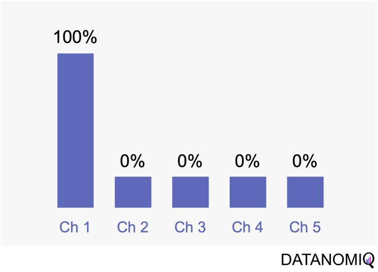
How Do Various Actor-Critic Based Deep Reinforcement Learning Algorithms Perform on Stock Trading?

Deep Reinforcement Learning for Automated Stock Trading: An Ensemble Strategy

Abstract

Deep Reinforcement Learning (DRL) is a blooming field famous for addressing a wide scope of complex decision-making tasks. This article would introduce and summarize the paper “Deep Reinforcement Learning for Automated Stock Trading: An Ensemble Strategy”, and discuss how these actor-critic based DRL learning algorithms, Proximal Policy Optimization (PPO), Advantage Actor Critic (A2C), and Deep Deterministic Policy Gradient (DDPG), act to accomplish automated stock trading by boosting investment return.

1 Motivation and Related Technology

It has long been challenging to design a comprehensive strategy for capital allocation optimization in a complex and dynamic stock market. With development of Artificial Intelligence, machine learning coupled with fundamentals analysis and alternative data has been in trend and provides better performance than conventional methodologies. Reinforcement Learning (RL) as a branch of it, is able to learn from interactions with environment, during which the agent continuously absorbs information, takes actions, and learns to improve its policy regarding rewards or losses obtained. On top of that, DRL utilizes neural networks as function approximators to approximate the Q-value (the expected reward of each action) in RL, which in return adjusts RL for large-scale data learning.

In DRL, the critic-only approach is capable for solving discrete action space problems, calculating Q-value to learn the optimal action-selection policy. On the other side, the actor-only approach, used in continuous action space environments, directly learns the optimal policy itself. Combining both, the actor-critic algorithm simultaneously updates the actor network representing the policy, and critic network representing the value function. The critic estimates the value function, while the actor updates the policy guided by the critic with policy gradients.

Overview of reinforcement learning-based stock theory.

Figure 1: Overview of reinforcement learning-based stock theory.

2 Mathematical Modeling

2.1 Stock Trading Simulation

Given the stochastic nature of stock market, the trading process is modeled as a Markov Decision Process (MDP) as follows:

  • State s = [p, h, b]: a vector describing the current state of the portfolio consists of D stocks, includes stock prices vector p, the stock shares vector h, and the remaining balance b.
  • Action a: a vector of actions which are selling, buying, or holding (Fig.2), resulting in decreasing, increasing, and no change of shares h, respectively. The number of shares been transacted is recorded as k.
  • Reward r(s, a, s’): the reward of taking action a at state s and arriving at the new state s’.
  • Policy π(s): the trading strategy at state s, which is the probability distribution of actions.
  • Q-value : the expected reward of taking action a at state s following policy π.
A starting portfolio value with three actions result in three possible portfolios.

A starting portfolio value with three actions result in three possible portfolios. Note that “hold” may lead to different portfolio values due to the changing stock prices.

Besides, several assumptions and constraints are proposed for practice:

  • Market liquidity: the orders are rapidly executed at close prices.
  • Nonnegative balance: the balance at time t+1 after taking actions at t, equals to the original balance plus the proceeds of selling minus the spendings of buying:
  • Transaction cost: assume the transaction costs to be 0.1% of the value of each trade:
  • Risk-aversion: to control the risk of stock market crash caused by major emergencies, the financial turbulence index that measures extreme asset price movements is introduced:

    where  denotes the stock returns, µ and Σ are respectively the average and covariance of historical returns. When  exceeds a threshold, buying will be halted and the agent sells all shares. Trading will be resumed once  returns to normal level.

2.2 Trading Goal: Return Maximation

The goal is to design a trading strategy that raises agent’s total cumulative compensation given by the reward function:

and then considering the transition of the shares and the balance defined as:

the reward can be further decomposed:

where:

At inception, h and Q_{\pi}(s,a) are initialized to 0, while the policy π(s) is uniformly distributed among all actions. Afterwards, everything is updated through interacting with the stock market environment. By the Bellman Equation, Q_{\pi}(s_t, a_t) is the expectation of the sum of direct reward r(s_t,a_t,s_{t+1} and the future reqard Q_{\pi}(s{t+1}, a_{a+1}) at the next state discounted by a factor γ, resulting in the state-action value function:

2.3 Environment for Multiple Stocks

OpenAI gym is used to implement the multiple stocks trading environment and to train the agent.

  1. State Space: a vector [b_t, p_t, h_t, M_t, R_t, C_t, X_t] storing information about
    b_t: Portfolio balance
    p_t: Adjusted close prices
    h_t: Shares owned of each stock
    M_t: Moving Average Convergence Divergence
    R_t: Relative Strength Index
    C_t: Commodity Channel Index
    X_t: Average Directional Index
  2. Action Space: {−k, …, −1, 0, 1, …, k} for a single stock, whose elements representing the number of shares to buy or sell. The action space is then normalized to [−1, 1], since A2C and PPO are defined directly on a Gaussian distribution.
Overview of the load-on-demand technique.

Overview of the load-on-demand technique.

Furthermore, a load-on-demand technique is applied for efficient use of memory as shown above.

  1. Algorithms Selection

This paper mainly uses the following three actor-critic algorithms:

  • A2C: uses parallel copies of the same agent to update gradients for different data samples, and a coordinator to pass the average gradients over all agents to a global network, which can update the actor and the critic network, with the objective function:
  • where \pi_{\theta}(a_t|s_t) is the policy network, and A(S_t|a_t) is the advantage function to reduce the high variance of it:
  • V(S_t)is the value function of state S_t, regardless of actions. DDPG: combines the frameworks of Q-learning and policy gradients and uses neural networks as function approximators; it learns directly from the observations through policy gradient and deterministically map states to actions. The Q-value is updated by:
    Critic network is then updated by minimizing the loss function:
  • PPO: controls the policy gradient update to ensure that the new policy does not differ too much from the previous policy, with the estimated advantage function and a probability ratio:

    The clipped surrogate objective function:

    takes the minimum of the clipped and normal objective to restrict the policy update at each step and improve the stability of the policy.

An ensemble strategy is finally proposed to combine the three agents together to build a robust trading strategy. After training and testing the three agents concurrently, in the trading stage, the agent with the highest Sharpe ratio in one period will be automatically selected to use in the next period.

  1. Implementation: Training and Validation

The historical daily trading data comes from the 30 DJIA constituent stocks.

Stock data splitting in-sample and out-of-sample

Stock data splitting in-sample and out-of-sample.

  • In-sample training stage: data from 01/01/2009 – 09/30/2015 used to train 3 agents using PPO, A2C, and DDPG;
  • In-sample validation stage: data from 10/01/2015 – 12/31/2015 used to validate the 3 agents by 5 metrics: cumulative return, annualized return, annualized volatility, Sharpe ratio, and max drawdown; tune key parameters like learning rate and number of episodes;
  • Out-of-sample trading stage: unseen data from 01/01/2016 – 05/08/2020 to evaluate the profitability of algorithms while continuing training. In each quarter, the agent with the highest Sharpe ratio is selected to act in the next quarter, as shown below.

    Table 1 - Sharpe Ratios over time.

    Table 1 – Sharpe Ratios over time.

  1. Results Analysis and Conclusion

From Table II and Fig.5, one can notice that PPO agent is good at following trend and performs well in chasing for returns, with the highest cumulative return 83.0% and annual return 15.0% among the three agents, indicating its appropriateness in a bullish market. A2C agent is more adaptive to handle risk, with the lowest annual volatility 10.4% and max drawdown −10.2%, suggesting its capability in a bearish market. DDPG generates the lowest return among the three, but works fine under risk, with lower annual volatility and max drawdown than PPO. Apparently all three agents outperform the two benchmarks.

Table 2 - Performance Evaluation Comparison.

Table 2 – Performance Evaluation Comparison.

Moreover, it is obvious in Fig.6 that the ensemble strategy and the three agents act well during the 2020 stock market crash, when the agents successfully stops trading, thus cutting losses.

Performance during the stock market crash in the first quarter of 2020.

Performance during the stock market crash in the first quarter of 2020.

From the results, the ensemble strategy demonstrates satisfactory returns and lowest volatilities. Although its cumulative returns are lower than PPO, it has achieved the highest Sharpe ratio 1.30 among all strategies. It is reasonable that the ensemble strategy indeed performs better than the individual algorithms and baselines, since it works in a way each elemental algorithm is supplementary to others while balancing risk and return.

For further improvement, it will be inspiring to explore more models such as Asynchronous Advantage Actor-Critic (A3C) or Twin Delayed DDPG (TD3), and to take more fundamental analysis indicators or ESG factors into consideration. While more sophisticated models and larger datasets are adopted, improvement of efficiency may also be a challenge.

Automated product quality monitoring using artificial intelligence deep learning

How to maintain product quality with deep learning

Deep Learning helps companies to automate operative processes in many areas. Industrial companies in particular also benefit from product quality assurance by automated failure and defect detection. Computer Vision enables automation to identify scratches and cracks on product item surfaces. You will find more information about how this works in the following infografic from DATANOMIQ and pixolution you can download using the link below.

How to maintain product quality with automatic defect detection - Infographic

How to maintain product quality with automatic defect detection – Infographic

Deep Autoregressive Models

Deep Autoregressive Models

In this blog article, we will discuss about deep autoregressive generative models (AGM). Autoregressive models were originated from economics and social science literature on time-series data where obser- vations from the previous steps are used to predict the value at the current and at future time steps [SS05]. Autoregression models can be expressed as:

    \begin{equation*} x_{t+1}= \sum_i^t \alpha_i x_{t-i} + c_i, \end{equation*}

where the terms \alpha and c are constants to define the contributions of previous samples x_i for the future value prediction. In the other words, autoregressive deep generative models are directed and fully observed models where outcome of the data completely depends on the previous data points as shown in Figure 1.

Autoregressive directed graph.

Figure 1: Autoregressive directed graph.

Let’s consider x \sim X, where X is a set of images and each images is n-dimensional (n pixels). Then the prediction of new data pixel will be depending all the previously predicted pixels (Figure ?? shows the one row of pixels from an image). Referring to our last blog, deep generative models (DGMs) aim to learn the data distribution p_\theta(x) of the given training data and by following the chain rule of the probability, we can express it as:

(1)   \begin{equation*} p_\theta(x) = \prod_{i=1}^n p_\theta(x_i | x_1, x_2, \dots , x_{i-1}) \end{equation*}

The above equation modeling the data distribution explicitly based on the pixel conditionals, which are tractable (exact likelihood estimation). The right hand side of the above equation is a complex distribution and can be represented by any possible distribution of n random variables. On the other hand, these kind of representation can have exponential space complexity. Therefore, in autoregressive generative models (AGM), these conditionals are approximated/parameterized by neural networks.

Training

As AGMs are based on tractable likelihood estimation, during the training process these methods maximize the likelihood of images over the given training data X and it can be expressed as:

(2)   \begin{equation*} \max_{\theta} \sum_{x\sim X} log \: p_\theta (x) = \max_{\theta} \sum_{x\sim X} \sum_{i=1}^n log \: p_\theta (x_i | x_1, x_2, \dots, x_{i-1}) \end{equation*}

The above expression is appearing because of the fact that DGMs try to minimize the distance between the distribution of the training data and the distribution of the generated data (please refer to our last blog). The distance between two distribution can be computed using KL-divergence:

(3)   \begin{equation*} \min_{\theta} d_{KL}(p_d (x),p_\theta (x)) = log\: p_d(x) - log \: p_\theta(x) \end{equation*}

In the above equation the term p_d(x) does not depend on \theta, therefore, whole equation can be shortened to Equation 2, which represents the MLE (maximum likelihood estimation) objective to learn the model parameter \theta by maximizing the log likelihood of the training images X. From implementation point of view, the MLE objective can be optimized using the variations of stochastic gradient (ADAM, RMSProp, etc.) on mini-batches.

Network Architectures

As we are discussing deep generative models, here, we would like to discuss the deep aspect of AGMs. The parameterization of the conditionals mentioned in Equation 1 can be realized by different kind of network architectures. In the literature, several network architectures are proposed to increase their receptive fields and memory, allowing more complex distributions to be learned. Here, we are mentioning a couple of well known architectures, which are widely used in deep AGMs:

  1. Fully-visible sigmoid belief network (FVSBN): FVSBN is the simplest network without any hidden units and it is a linear combination of the input elements followed by a sigmoid function to keep output between 0 and 1. The positive aspects of this network is simple design and the total number of parameters in the model is quadratic which is much smaller compared to exponential [GHCC15].
  2. Neural autoregressive density estimator (NADE): To increase the effectiveness of FVSBN, the simplest idea would be to use one hidden layer neural network instead of logistic regression. NADE is an alternate MLP-based parameterization and more effective compared to FVSBN [LM11].
  3. Masked autoencoder density distribution (MADE): Here, the standard autoencoder neural networks are modified such that it works as an efficient generative models. MADE masks the parameters to follow the autoregressive property, where the current sample is reconstructed using previous samples in a given ordering [GGML15].
  4. PixelRNN/PixelCNN: These architecture are introducced by Google Deepmind in 2016 and utilizing the sequential property of the AGMs with recurrent and convolutional neural networks.
Different autoregressive architectures

Figure 2: Different autoregressive architectures (image source from [LM11]).

Results using different architectures

Results using different architectures (images source https://deepgenerativemodels.github.io).

It uses two different RNN architectures (Unidirectional LSTM and Bidirectional LSTM) to generate pixels horizontally and horizontally-vertically respectively. Furthermore, it ulizes residual connection to speed up the convergence and masked convolution to condition the different channels of images. PixelCNN applies several convolutional layers to preserve spatial resolution and increase the receptive fields. Furthermore, masking is applied to use only the previous pixels. PixelCNN is faster in training compared to PixelRNN. However, the outcome quality is better with PixelRNN [vdOKK16].

Summary

In this blog article, we discussed about deep autoregressive models in details with the mathematical foundation. Furthermore, we discussed about the training procedure including the summary of different network architectures. We did not discuss network architectures in details, we would continue the discussion of PixelCNN and its variations in upcoming blogs.

References

[GGML15] Mathieu Germain, Karol Gregor, Iain Murray, and Hugo Larochelle. MADE: masked autoencoder for distribution estimation. CoRR, abs/1502.03509, 2015.

[GHCC15] Zhe Gan, Ricardo Henao, David Carlson, and Lawrence Carin. Learning Deep Sigmoid Belief Networks with Data Augmentation. In Guy Lebanon and S. V. N. Vishwanathan, editors, Proceedings of the Eighteenth International Conference on Artificial Intelligence
and Statistics, volume 38 of Proceedings of Machine Learning Research, pages 268–276, San Diego, California, USA, 09–12 May 2015. PMLR.

[LM11] Hugo Larochelle and Iain Murray. The neural autoregressive distribution estimator. In Geoffrey Gordon, David Dunson, and Miroslav Dudík, editors, Proceedings of the Fourteenth International Conference on Artificial Intelligence and Statistics, volume 15 of Proceedings of Machine Learning Research, pages 29–37, Fort Lauderdale, FL, USA, 11–13 Apr 2011.
PMLR.

[SS05] Robert H. Shumway and David S. Stoffer. Time Series Analysis and Its Applications (Springer Texts in Statistics). Springer-Verlag, Berlin, Heidelberg, 2005.

[vdOKK16] A ̈aron van den Oord, Nal Kalchbrenner, and Koray Kavukcuoglu. Pixel recurrent neural
networks. CoRR, abs/1601.06759, 2016

How to ensure occupational safety using Deep Learning – Infographic

In cooperation between DATANOMIQ, my consulting company for data science, business intelligence and process mining, and Pixolution, a specialist for computer vision with deep learning, we have created an infographic (PDF) about a very special use case for companies with deep learning: How to ensure occupational safety through automatic risk detection using using Deep Learning AI.

How to ensure occupational safety through automatic risk detection using Deep Learning - Infographic

How to ensure occupational safety through automatic risk detection using Deep Learning – Infographic