1 Overview
Development of computer processing power, network and automated software completely change and give new concept of each business. And data mining play the vital part to solve, finding the hidden patterns and relationship from large dataset with business by using sophisticated data analysis tools like methodology, method, process flow etc.
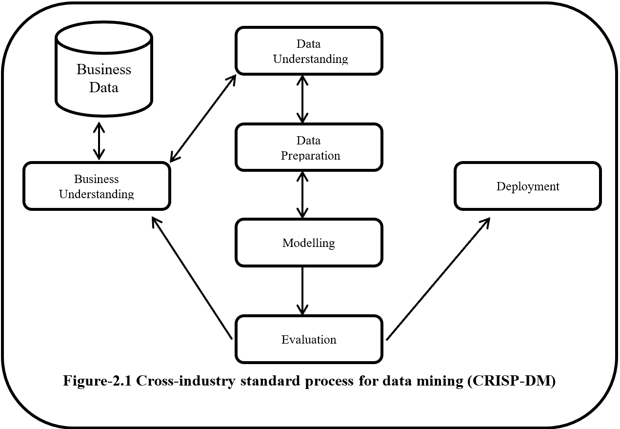
On this paper, proposed a process flow followed CRISP-DM methodology and has six steps where data understanding does not considered.
Phase of new process flow given below:-
Phase 1: Involved with collection, outliner treatment, imputation, transformation, scaling, and partition dataset in to two sub-frames (Training and Testing). Here as an example for outliner treatment, imputation, transformation, scaling consider accordingly Z score, mean, One hot encoding and Min Max Scaler.
Phase 2: On this Phase training and testing data balance with same balancing algorithm but separately. As an example here SMOTE (synthetic minority oversampling technique) is considered.
Phase 3: This phase involved with reduction, selection, aggregation, extraction. But here for an example considering same feature reduction algorithm (LDA -Linear Discriminant analysis) on training and testing data set separately.
Phase 4: On this Phase Training data set again partition into two more set (Training and Validation).
Phase 5: This Phase considering several base algorithms as a base model like CNN, RNN, Random forest, MLP, Regression, Ensemble method. This phase also involve to find out best hyper parameter and sub-algorithm for each base algorithm. As an example on this paper consider two class classification problems and also consider Random forest (Included CART – Classification and Regression Tree and GINI index impurity) and MLP classifier (Included (Relu, Sigmoid, binary cross entropy, Adam – Adaptive Moment Estimation) as base algorithms.
Phase 6: First, Prediction with validation data then evaluates with Test dataset which is fully unknown for these (Random forest, MLP classifier) two base algorithms. Then calculate the confusion matrix, ROC, AUC to find the best base algorithm.
New method from phase 1 to phase 4 followed CRISP-DM methodology steps such as data collection, data preparation then phase 5 followed modelling and phase 6 followed evaluation and implementation steps.
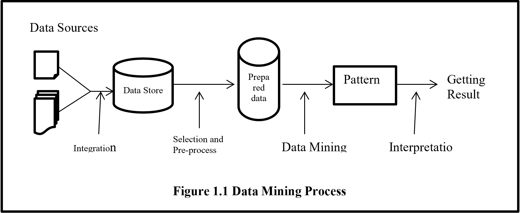
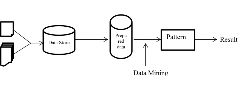
Structure of proposed process flow for two class problem combined with algorithm and sub-algorithm display on figure – 1.
These articles mainly focus to describe all algorithms which are going to implementation for better understanding.
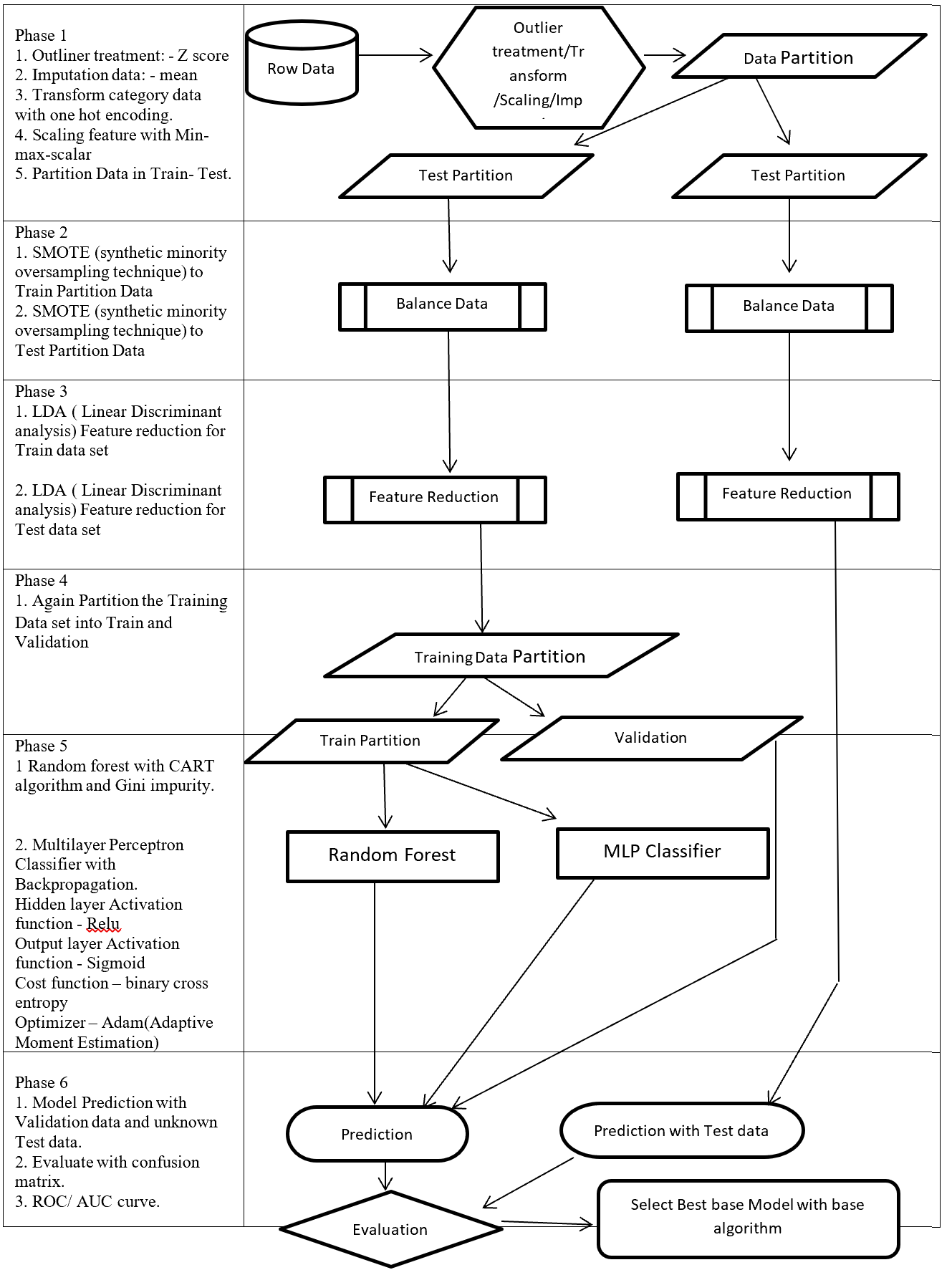
Figure 1 – Data Mining Process Flow
2 Phase 1: Outlier treatment, Transform, Scaling, Imputation
This phase involved with outlier treatment, imputation, scaling, and transform data.
2.1 Outliner treatment: – Z score
Outlier is a data point which lies far from all other data point in a data set. Outlier need to treat because it may bias the entire result. Outlier treatment with Z score is a common technique. Z score is a standard score in statistics. Z score provides information about data value is smaller or grater then mean that means how many standard deviations away from the mean value. Z score equation display below:

Here x = data point
σ = Standard deviation
μ = mean value
Equation- 1 Z-Score
In a normal distribution Z score represent 68% data lies on +/- 1, 95% data point lies on +/- 2, 99.7% data point lies on +/- 3 standard deviation.
2.2 Imputation data: – mean
Imputation is a way to handle missing data by replacing substituted value. There are many imputation technique represent like mean, median, mode, k-nearest neighbours. Mean imputation is the technique to replacing missing information with mean value. On the mean imputation first calculate the particular features mean value and then replace the missing value with mean value. The next equation displays the mean calculation:

Here x = value of each point
n = number of values
μ = mean value
Equation- 2 Mean
2.3 Transform: – One hot encoding
Encoding is a pre-processing technique which represents data in such a way that computer can understand. For understanding of machine learning algorithm categorical columns convert to numerical columns, this process called categorical encoding. There are multiple way to handle categorical variable but most widely used techniques are label encoding and one host encoding. On label encoding give a numeric (integer number) for each category. Suppose there are 3 categories of foods like apples, orange, banana. When label encoding is used then 3 categories will get a numerical value like apples = 1, banana = 2 and orange = 3. But there is very high probability that machine learning model can capture the relationship in between categories such as apple < banana < orange or calculate average across categories like 1 +3 = 4 / 2 = 2 that means model can understand average of apple and orange together is banana which is not acceptable because model correlation calculation is wrong. For solving this problem one hot encoding appear. The following table displays the label encoding is transformed into one hot encoding.
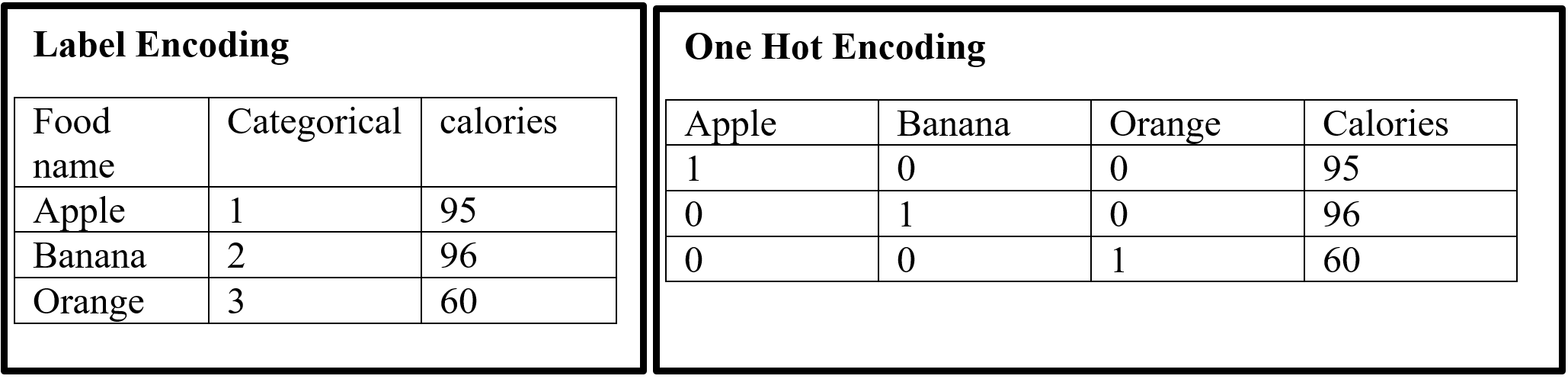
Table- 1 Encoding example
On hot encoding categorical value split into columns and each column contains 0 or 1 according to columns placement.
2.4 Scaling data: – Min Max Scaler
Feature scaling method is standardized or normalization the independent variable that means it is used to scale the data in a particular range like -1 to +1 or depending on algorithm. Generally normalization used where data distribution does not follow Gaussian distribution and standardization used where data distribution follow Gaussian distribution. On standardization techniques transform data values are cantered around the mean and unit is standard deviation. Formula for standardization given below:

Equation-3 Equations for Standardization
X represent the feature value, µ represent mean of the feature value and σ represent standard deviation of the feature value. Standardized data value does not restrict to a particular range.
Normalization techniques shifted and rescaled data value range between 0 and 1. Normalization techniques also called Min-Max scaling. Formula for normalization given below:

Equation – 4 Equations for Normalization
Above X, Xmin, Xmax are accordingly feature values, feature minimum value and feature maximum value. On above formula when X is minimums then numerator will be 0 ( is 0) or if X is maximums then the numerator is equal to the denominator ( is 1). But when X data value between minimum and maximum then is between 0 and 1. If ranges value of data does not normalized then bigger range can influence the result.
3 Phase 2: – Balance Data
3.1 SMOTE
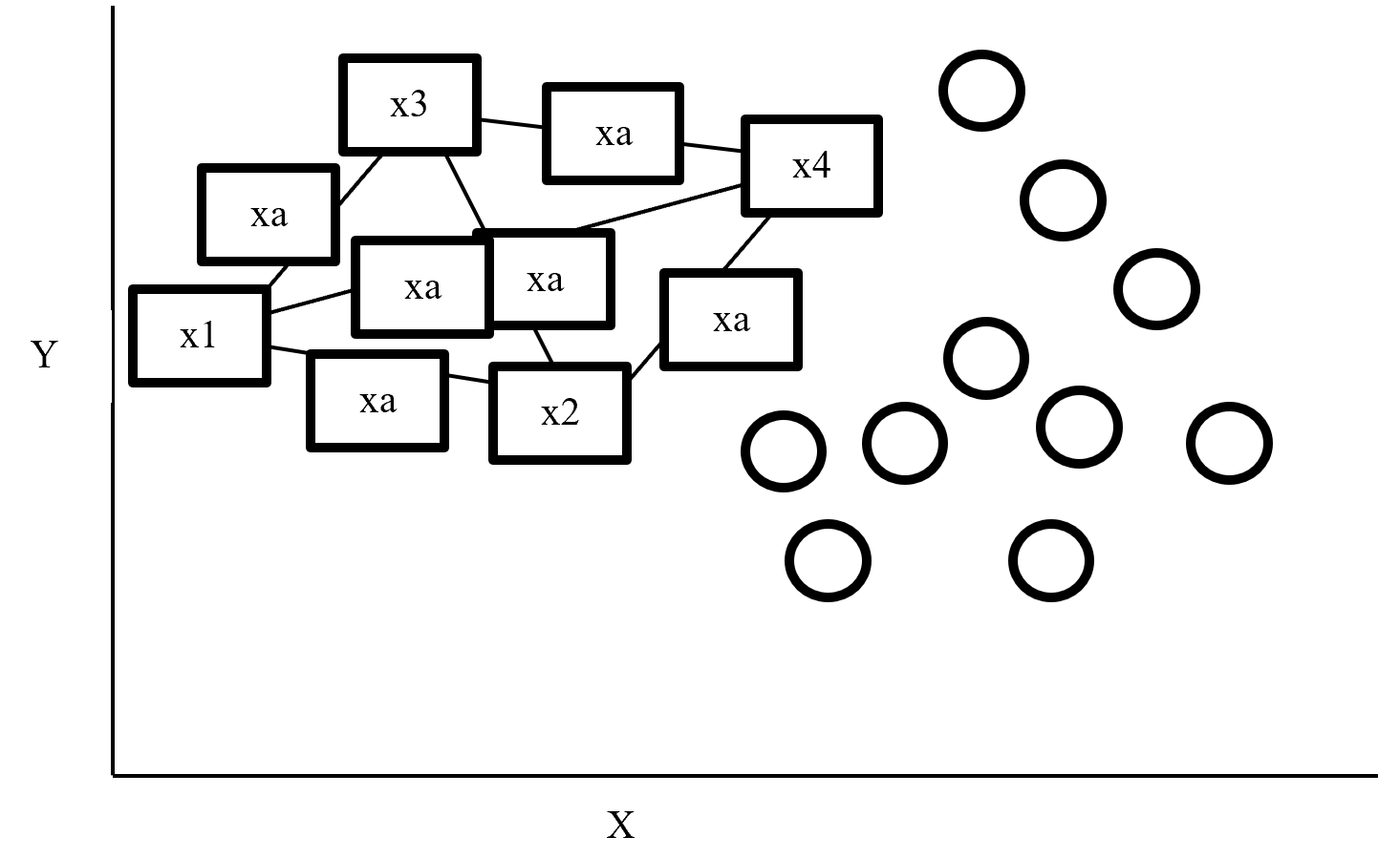
SMOTE (synthetic minority oversampling technique) is an oversampling technique where synthetic observations are created based on existing minority observations. This technique operates in feature space instead of data space. Under SMOTE each minority class observation calculates k nearest neighbours and randomly chose the neighbours depending on over-sampling requirements. Suppose there are 4 data point on minority class and 10 data point on majority class. For this imbalance data set, balance by increasing minority class with synthetic data point. SMOTE creating synthetic data point but it is necessary to consider k nearest neighbours first. If k = 3 then SMOTE consider 3 nearest neighbours. Figure-2 display SMOTE with k = 3 and x = x1, x2, x3, x4 data point denote minority class. And all circles represent majority class.

Figure- 2 SMOTE example
4 Phase 3: – Feature Reduction
4.1 LDA
LDA stands for Linear Discriminant analysis supervised technique are commonly used for classification problem. On this feature reduction account continuous independent variable and output categorical variable. It is multivariate analysis technique. LDA analyse by comparing mean of the variables. Main goal of LDA is differentiate classes in low dimension space. LDA is similar to PCA (Principal component analysis) but in addition LDA maximize the separation between multiple classes. LDA is a dimensionality reduction technique where creating synthetic feature from linear combination of original data set then discard less important feature. LDA calculate class variance, it maximize between class variance and minimize within class variance. Table-2 display the process steps of LDA.
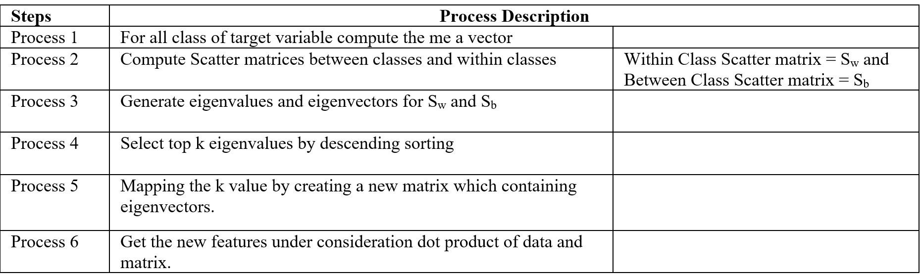
Table- 2 LDA process
5 Phase 5: – Base Model
Here we consider two base model ensemble random forest and MLP classifier.
5.1 Random Forest
Random forest is an ensemble (Bagging) method where group of weak learner (decision tree) come together to form a strong leaner. Random forest is a supervised algorithm which is used for regression and classification problem. Random forests create several decisions tree for predictions and provide solution by voting (classification) or mean (regression) value. Working process of Random forest given below (Table -3).
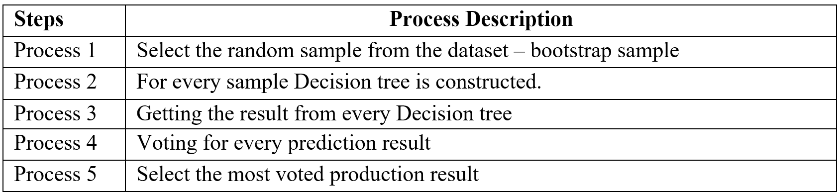
Table-3 Random Forest process
When training a Random forest root node contains a sample of bootstrap dataset and the feature is as same as original dataset. Suppose the dataset is D and contain d record and m number of columns. From the dataset D random forest first randomly select sample of rows (d’) with replacement and sample of features (n’) and give it to the decision tree. Suppose Random forest created several decision trees like T1, T2, T3, T4 . . . Tn. Then randomly selected dataset D’ = d’ + n’ is given to the decision tree T1, T2, T3, T4 . . . Tn where D’ < D, m > n’ and d > d’. After taking the dataset decision tree give the prediction for binary classification 1 or 0 then aggregating the decision and select the majority voted result. Figure-3 describes the structure of random forest process.
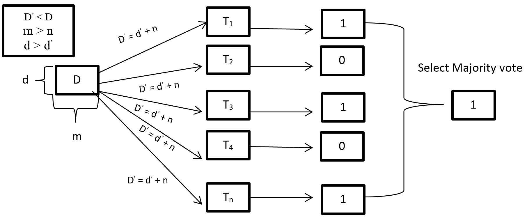
Figure- 3 Random Forest process
On Random forest base learner Decision Tree grows complete depth where bias (properly train on training dataset) is low and variance is high (when implementing test data give big error) called overfitting. On Random forest using multiple decision trees where each Decision tree is high variance but when combining all decision trees with the respect of majority vote then high variance converted into low variance because using row and feature sampling with replacement and taking the majority vote where decision is not depend on one decision tree.
CART (Classification and Regression Tree) is binary segmentation technique. CART is a Gini’s impurity index based classical algorithm to split a dataset and build a decision tree. By splitting a selected dataset CART created two child nodes repeatedly and builds a tree until the data no longer be split. There are three steps CART algorithm follow:
- Find best split for each features. For each feature in binary split make two groups of the ordered classes. That means possibility of split for k classes is k-1. Find which split is maximized and contain best splits (one for each feature) result.
- Find the best split for nodes. From step 1 find the best one split (from all features) which maximized the splitting criterion.
- Split the best node from step 2 and repeat from step 1 until fulfil the stopping criterion.
For splitting criteria CART use GINI index impurity algorithm to calculate the purity of split in a decision tree. Gini impurity randomly classified the labels with the same distribution in the dataset. A Gini impurity of 0 (lowest) is the best possible impurity and it is achieve when everything is in a same class. Gini index varies from 0 to 1. 0 indicate the purity of class where only one class exits or all element under a specific class. 1 indicates that elements are randomly distributed across various classes. And 0.5 indicate equal elements distributed over classes. Gini index (GI) described by mathematically that sum of squared of probabilities of each class (pi) deducted from one (Equation-5).

Equation – 5 Gini impurities
Here (Equation-5) pi represent the probability (probability of p+ or yes and probability of p- or no) of distinct class with classified element. Suppose randomly selected feature (a1) which has 8 yes and 4 no. After the split right had side (b1 on equation-6) has 4 yes and 4 no and left had side (b2 on equation – 7) has 4 yes and 0 no. here b2 is a pure split (leaf node) because only one class yes is present. By using the GI (Gini index) formula for b1 and b2:-
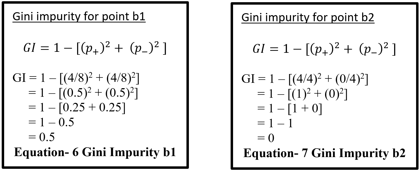
Equation- 6 & 7 – Gini Impurity b1 & Gini Impurity b2
Here for b1 value 0.5 indicates that equal element (yes and no) distribute over classes which is not pure split. And b2 value 0 indicates pure split. On GINI impurity indicates that when probability (yes or no) increases GINI value also increases. Here 0 indicate pure split and .5 indicate equal split that means worst situation. After calculating the GINI index for b1 and b2 now calculate the reduction of impurity for data point a1. Here total yes 8 (b1 and b2 on Equation – 8) and total no 4 (b1) so total data is 12 on a1. Below display the weighted GINI index for feature a1:
Total data point on b1 with Gini index (m) = 8/12 * 0.5 = 0.3333
Total data point on b2 with Gini index (n) = 4/12 * 0 = 0
Weighted Gini index for feature a1 = m + n = 0.3333
Equation- 8 Gini Impurity b1 & b2
After computing the weighted Gini value for every feature on a dataset taking the highest value feature as first node and split accordingly in a decision tree. Gini is less costly to compute.
5.2 Multilayer Perceptron Classifier (MLP Classifier)
Multilayer perceptron classifier is a feedforward neural network utilizes supervised learning technique (backpropagation) for training. MLP Classifier combines with multiple perceptron (hidden) layers. For feedforward taking input send combining with weight bias and then activation function from one hidden layer output goes to other hidden and this process continuing until reached the output. Then output calculates the error with error algorithm. These errors send back with backpropagation for weight adjustment by decreasing the total error and process is repeated, this process is call epoch. Number of epoch is determined with the hyper-parameter and reduction rate of total error.
5.2.1 Back-Propagation
Backpropagation is supervised learning algorithm that is used to train neural network. A neural network consists of input layer, hidden layer and output layer and each layer consists of neuron. So a neural network is a circuit of neurons. Backpropagation is a method to train multilayer neural network the updating of the weights of neural network and is done in such a way so that the error observed can be reduced here, error is only observed in the output layer and that error is back propagated to the previous layers and previous layer is proportionally updated weight. Backpropagation maintain chain rule to update weight. Mainly three steps on backpropagation are (Table-4):
| Step |
Process |
| Step 1 |
Forward Pass |
| Step 2 |
Backward Pass |
| Step 3 |
Sum of all values and calculate updated weight value with Chain – rules. |
Table-4 Back-Propagation process
5.2.2 Forward pass/ Forward propagation
Forward propagation is the process where input layer send the input value with randomly selected weight and bias to connected neuron and inside neuron selected activation function combine them and forward to other connected neuron layer after layer then give an output with the help of output layer. Below (Figure-4) display the forward propagation.
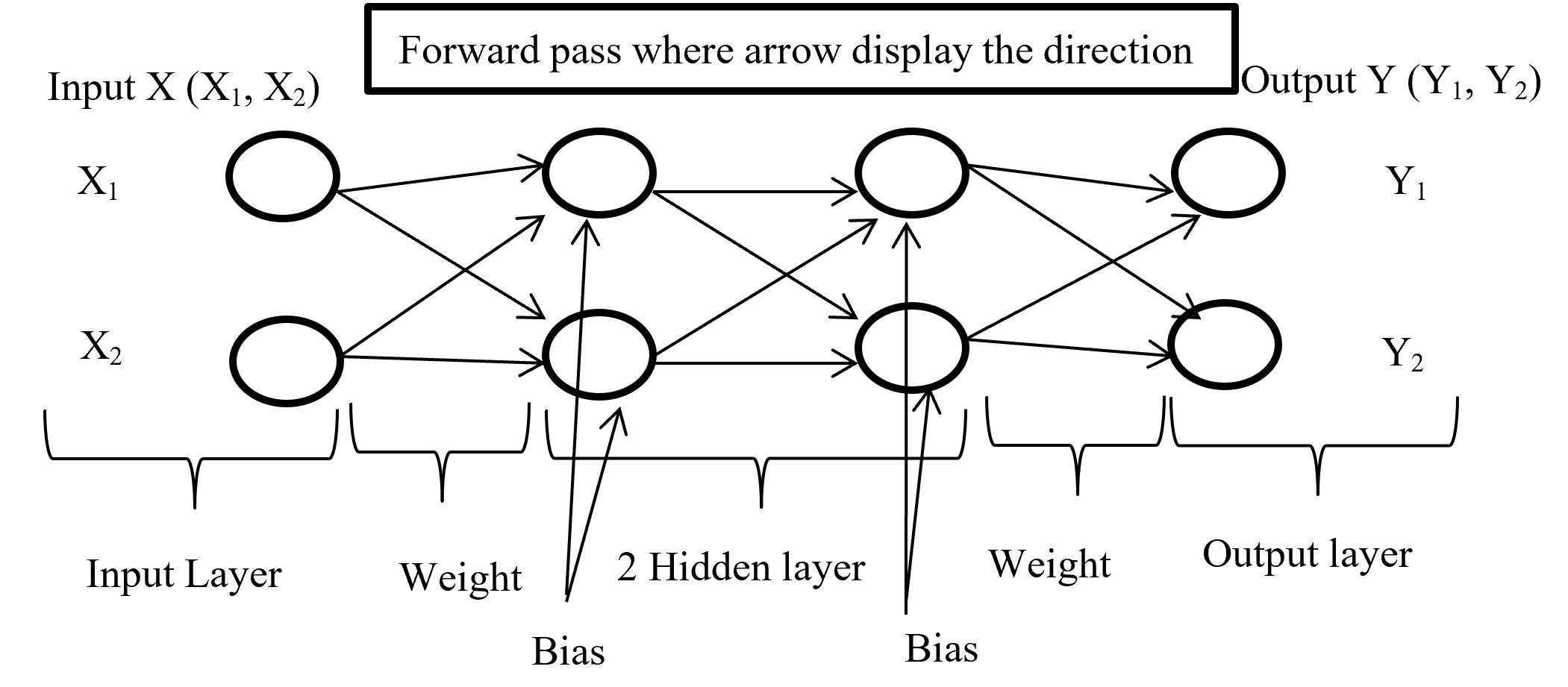
Figure-4 Forward passes
Input layer take the input of X (X1, X2) combine with randomly selected weight for each connection and with fixed bias (different hidden layer has different bias) send it to first hidden layer where first multiply the input with corresponding weight and added all input with single bias then selected activation function (may different form other layer) combine all input and give output according to function and this process is going on until reach in output layer. Output layer give the output like Y (Y1, Y2) (here output is binary classification as an example) according to selected activation function.
5.2.3 Backward Pass
After calculating error (difference between Forward pass output and actual output) backward pass try to minimize the error with optimisation function by sending backward with proportionally distribution and maintain a chain rule. Backward pass distribution the error in such a way where weighted value is taking under consideration. Below (Figure-5) diagram display the Backward pass process.
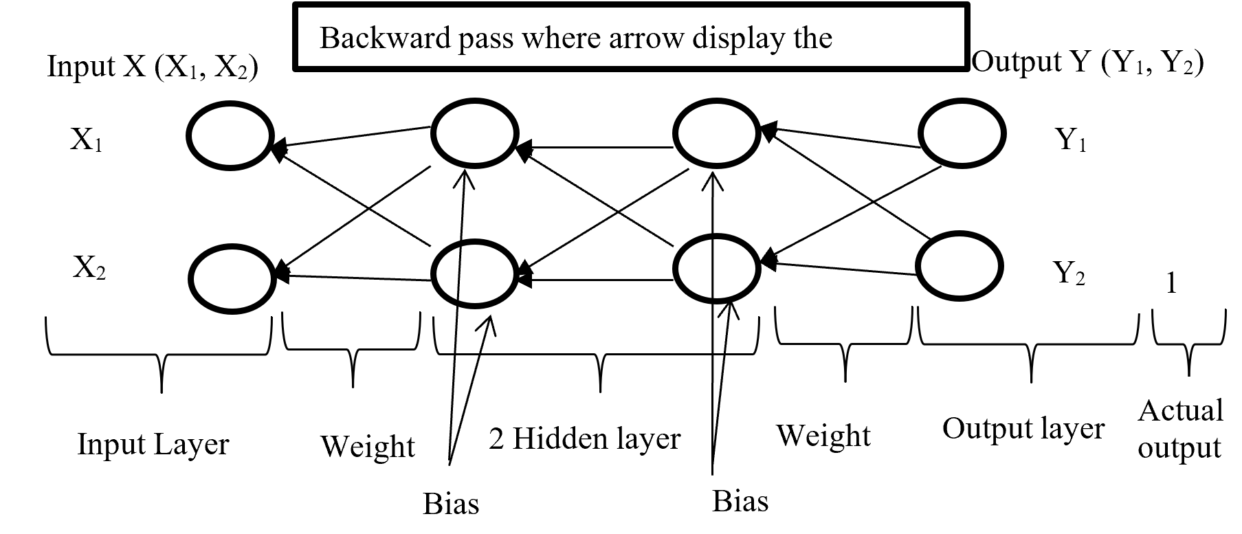
Figure-5 Backward passes
Backpropagation push back the error which is calculated with error function or loss function for update proportional distribution with the help of optimisation algorithm. Division of Optimisation algorithm given below on Figure – 6
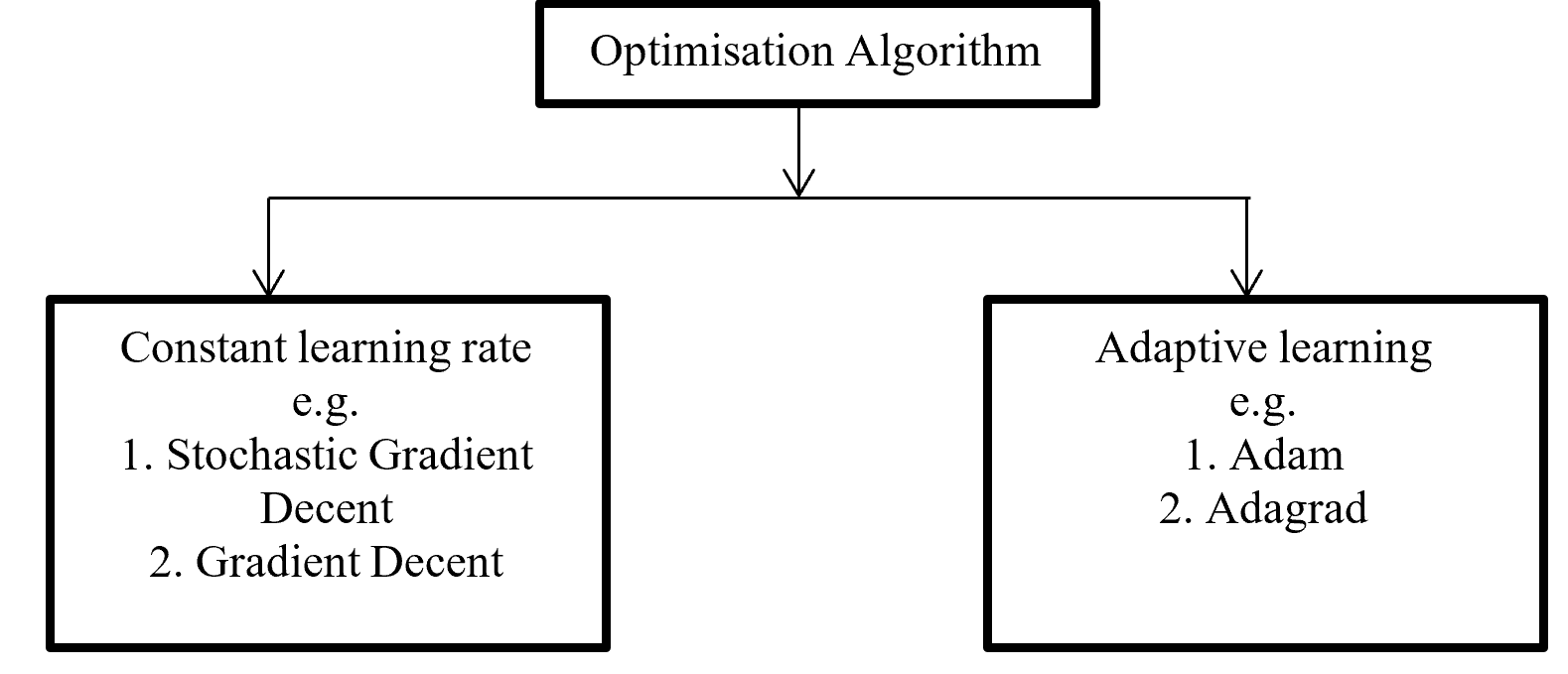
Figure -6 Division of Optimisation algorithms
Gradient decent calculate gradient and update value by increases or decreases opposite direction of gradients unit and try to find the minimal value. Gradient decent update just one time for whole dataset but stochastic gradient decent update on each training sample and it is faster than normal gradient decent. Gradient decent can be improve by tuning parameter like learning rate (0 to 1 mostly use 0.5). Adagrad use time step based parameter to compute learning rate for every parameter. Adam is Adaptive Moment Estimation. It calculates different parameter with different learning rate. It is faster and performance rate is higher than other optimization algorithm. On the other way Adam algorithm is squares the calculated exponential weighted moving average of gradient.
5.2.4 Chain – rules
Backpropagation maintain chain-rules to update weighted value. On chain-rules backpropagation find the derivative of error respect to any weight. Suppose E is output error. w is weight for input a and bias b and ac neuron output respect of activation function and summation of bias with weighted input (w*a) input to neuron is net. So partial derivative for error respect to weight is ∂E / ∂w display the process on figure-7.
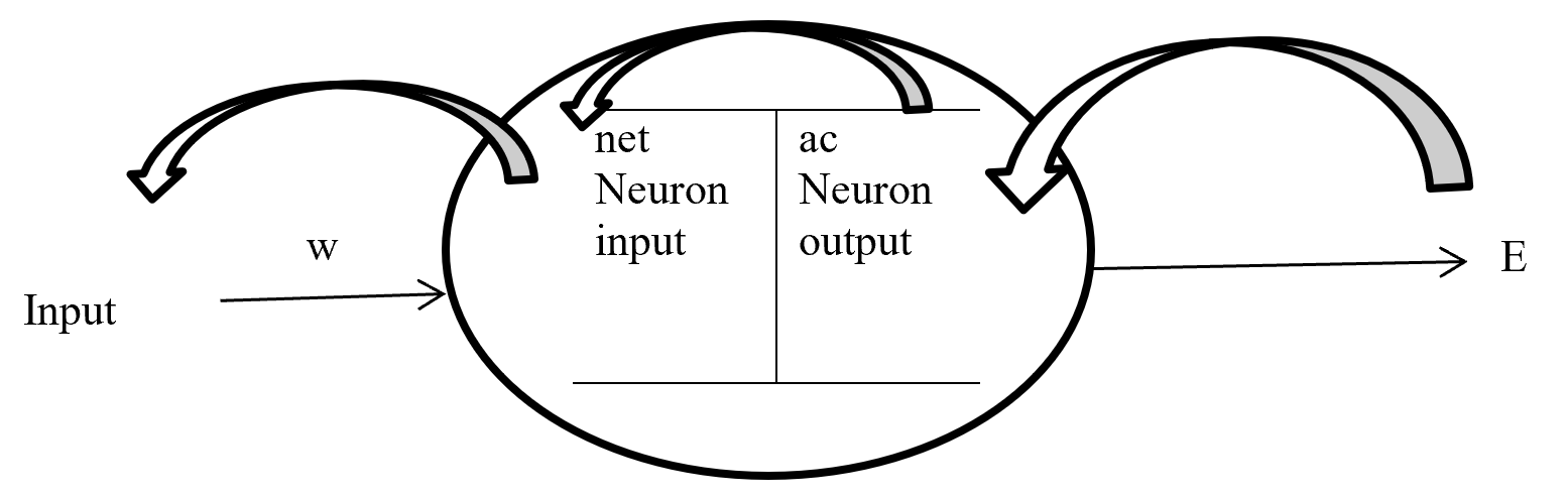
Figure- 7 Partial derivative for error respect to weight
On the chain rules for backward pass to find (error respect to weight) ∂E / ∂w = ∂E / ∂ac * ∂ac / ∂net * ∂net / ∂w. here find to error respect to weight are error respect to output of activation function multiply by activation function output respect to input in a neuron multiply by input in a neuron respect to weight.
5.2.5 Activation function
Activation function is a function which takes the decision about neuron to activate or deactivate. If the activate function activate the neuron then it will give an output on the basis of input. Input in a activation function is sum of input multiply with corresponding weight and adding the layered bias. The main function of a activate function is non-linearity output of a neuron.
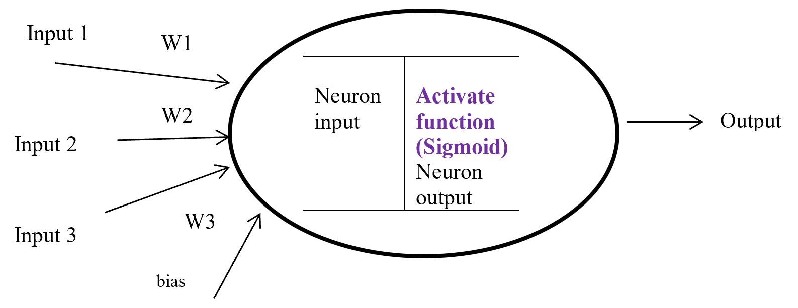
Figure-8 Activation function
Figure – 8 display a neuron in a hidden layer. Here several input (1, 2, 3) with corresponding weight (w1, w2, w3) putting in a neuron input layer where layer bias add with summation of multiplication with input and weight. Equation-9 display the output of an activate function.
Output from activate function y = Activate function (Ʃ (weight * input) + bias)
y = f (Ʃ (w*x) +b)
Equation- 9 Activate function
There are many activation functions like linear function for regression problem, sigmoid function for binary classification problem where result either 0 or 1, Tanh function which is based on sigmoid function but mathematically shifted version and values line -1 to 1. RELU function is Rectified linear unit. RELU is less expensive to compute.
5.2.6 Sigmoid
Sigmoid is a squashing activate function where output range between 0 and 1. Sigmoidal name comes from Greek letter sigma which looks like letter S when graphed. Sigmoid function is a logistic type function, it mainly use in output layer in neural network. Sigmoid is non-linear, fixed output range (between 0 and 1), monotonic (never decrees or never increases) and continuously differentiated function. Sigmoid function is good at classification and output from sigmoid is nonlinear. But Sigmoid has a vanishing gradient problem because output variable is very less to change in input variable. Figure- 9 displays the output of a Sigmoid and derivative of Sigmoid. Here x is any number (positive or negative). On sigmoid function 1 is divided by exponential negative input with adding 1.
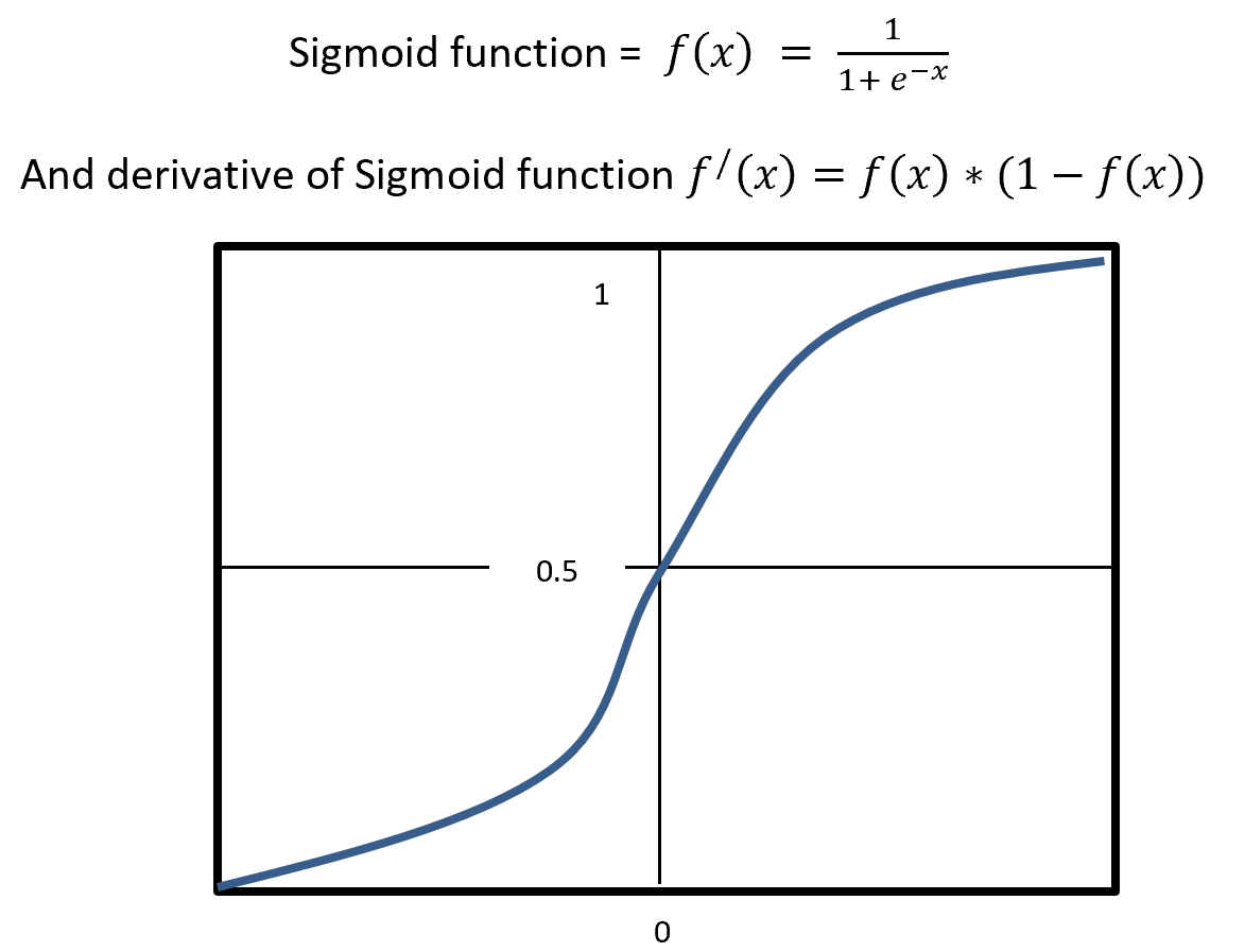
Figure – 9 Sigmoid Functions
4.5.2.7 RELU
RELU stands for Rectified Linear Units it is simple, less expensive in computation and rectifies the gradient vanishing problem. RELU is nonlinear activation function. It gives output either positive (infinity) or 0. RELU has a dying problem because if neurons stop for responding to variation because of gradient is 0 or nothing has to change. Figure- 10 displays the output of an RELU and derivative of RELU. Here x is any positive input and if x is grater then 0 give the output as x or give output 0. RELU function gives the output maximum value of input, here max (0, x).
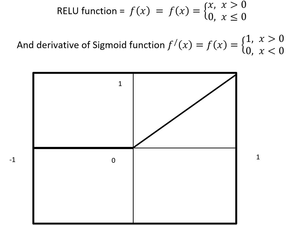
Figure – 10 RELU Function
4.5.2.8 Cost / loss function (Binary Cross-Entropy)
Cost or loss function compare the predictive value (model outcome) with actual value and give a quantitative value which give the indication about how much good or bad the prediction is.
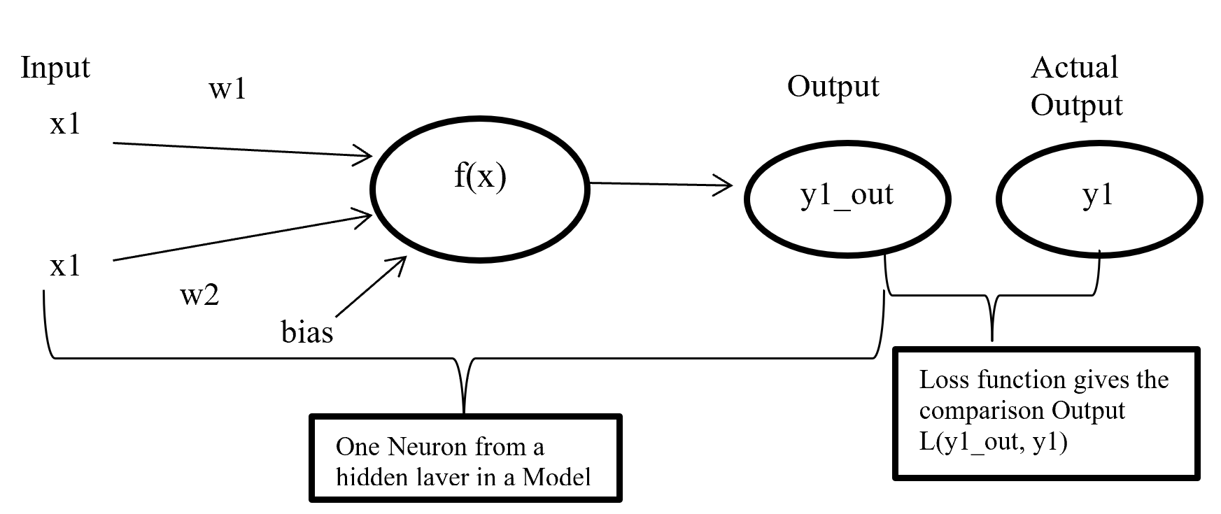
Figure- 11 Cost function work process
Figure-11 x1 and x2 are input in a activate function f(x) and output y1_out which is sum of weighted input added with bias going through activate function. After model output activate function compare the output with actual output and give a quantitative value which indicate how good or bad the prediction is.
There are many type of loss function but choosing of optimal loss function depends on the problem going to be solved such as regression or classification. For binary classification problem binary cross entropy is used to calculate cost. Equation-10 displays the binary cross entropy where y is actual binary value and yp predictive outcome range 0 and 1. And i is scalar vale range between 1 to model output size (N).
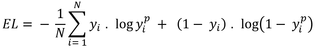
Equation-10 displays the binary cross entropy
6 Phase 6: – Evaluation
6.1 Confusion matrix
In a classification confusion matrix describe the performance of actual value against predictive value. Confusion Matrix does the performance measurement. So confusion matrix classifies and display predicted and actual value (Visa, S., Ramsay 2011).
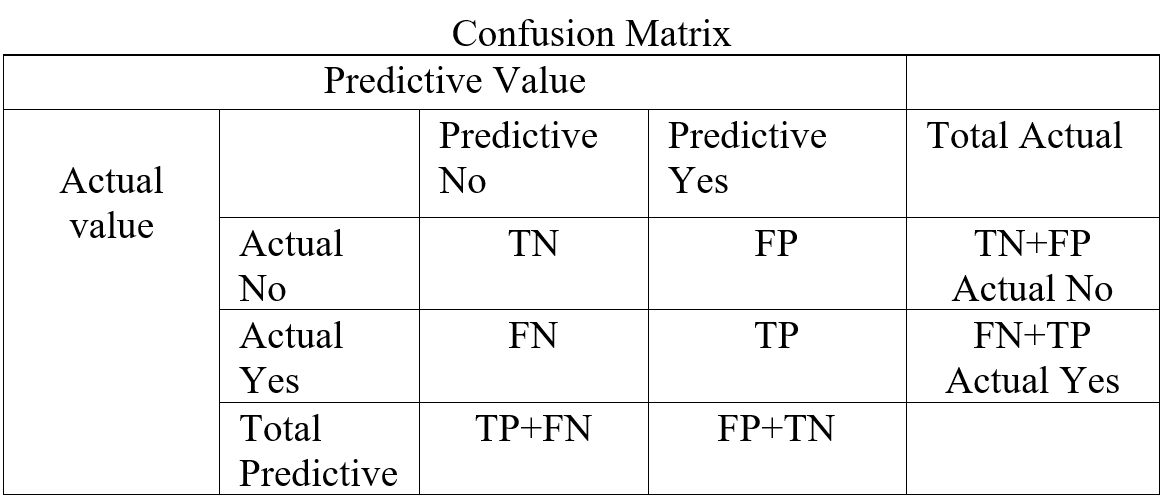
Table- 5 Confusion Matrix
Confusion Matrix (Table-5) combines with True Positive (TP), True Negative (TN), False Positive (FP), and False Negative (FN). True Positive is prediction positive and true. True Negative is prediction negative and that is true. False positive is prediction positive and it’s false. False negative is prediction negative and that is false. False positive is known as Type1 error and false negative is known as Type 2 error. Confusion matrix can able to calculate several list of rates which are given below on Table- 6.
Here N = Total number of observation, TP = True Positive, TN = True Negative
FP = False Positive, FN = False Negative, Total Actual No (AN) = TN + FP,
Total Predictive Yes (PY) = FP + TP. Total Actual Yes (AY) = FN + TP
| Rate
|
Description |
Mathematical Description |
| Accuracy |
Classifier, overall how often correctly identified |
(TP+TN) / N |
| Misclassification Rate |
Classifier, overall how often wrongly identified |
(FP + FN) / N |
| True Positive Rate
(Sensitivity / Recall) |
Classifier, how often predict correctly yes when it is actually yes. |
TP / AY |
| False Positive Rate |
Classifier, how often predict wrongly yes when it is actually no. |
FP / AN |
| True Negative Rate
(Specificity) |
Classifier, how often predict correctly no when it is actually no. |
TN / AN |
| Precision |
Classifier how often predict yes when it is correct. |
TP / PY |
| Prevalence |
Yes conditions how often occur in a sample. |
AY / N |
Table – 6 Confusion matrixes Calculation
From confusion matrix F1 score can be calculated because F1 score related to precision and recall. Higher F1 score is better. If precision or recall any one goes down F1 score also go down.

4.6.2 ROC (Receiver Operating Characteristic) curve
In statistics ROC is represent in a graph with plotting a curve which describe a binary classifiers performance as its differentiation threshold is varied. ROC (Equation-11) curve created true positive rate (TPR) against false positive rate (FPR). True positive rate also called as Sensitivity and False positive rate also known as Probability of false alarm. False positive rate also called as a probability of false alarm and it is calculated as 1 – Specificity.


Equation- 11 ROC
So ROC (Receiver Operation Characteristic) curve allows visual representation between sensitivity and specificity associated with different values of the test result (Grzybowski, M. and Younger, J.G., 1997)
On ROC curve each point has different Threshold level. Below (Figure – 12) display the ROC curve. Higher the area curve covers is better that means high sensitivity and high specificity represent more accuracy. ROC curve also represent that if classifier predict more often true than it has more true positive and also more false positive. If classifier predict true less often then fewer false positive and also fewer true positive.
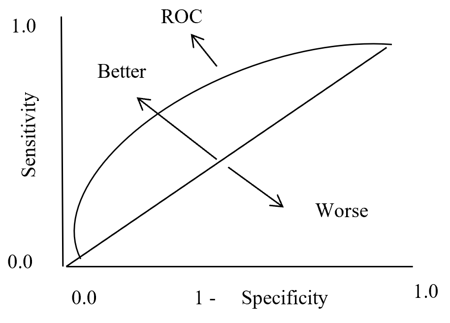
ROC Curve
Figure – 12 ROC curve description
4.6.3 AUC (Area under Curve)
Area under curve (AUC) is the area surrounded by the ROC curve and AUC also represent the degree of separability that means how good the model to distinguished between classes. Higher the AUC value represents better the model performance to separate classes. AUC = 1 for perfect classifier, AUC = 0 represent worst classifier, and AUC = 0.5 means has no class separation capacity. Suppose AUC value is 0.6 that means 60% chance that model can classify positive and negative class.
Figure- 13 to Figure – 16 displays an example of AUC where green distribution curve for positive class and blue distribution curve for negative class. Here threshold or cut-off value is 0.5 and range between ‘0’ to ‘1’. True negative = TN, True Positive = TP, False Negative = FN, False Positive = FP, True positive rate = TPR (range 0 to 1), False positive rate = FPR (range 0 to 1).
On Figure – 13 left distribution curve where two class curves does not overlap that means both class are perfectly distinguished. So this is ideal position and AUC value is 1. On the left side ROC also display that TPR for positive class is 100% occupied.
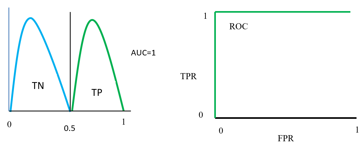
ROC distributions (perfectly distinguished
Figure – 14 two class overlap each other and raise false positive (Type 1), false negative (Type 2) errors. Here error could be minimize or maximize according to threshold. Suppose here AUC = 0.6, that means chance of a model to distinguish two classes is 60%. On ROC curve also display the curve occupied for positive class is 60%.

ROC distributions (class partly overlap distinguished)
Figure- 15 displayed that positive and negative overlap each other. Here AUC value is 0.5 or near to 0.5. On this position classifier model does not able distinguish positive and negative classes. On left side ROC curve become straight that means TPR and FPR are equal.
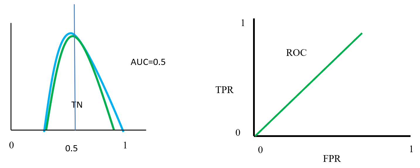
ROC distributions (class fully overlap distinguished)
Figure- 16 positive and negative class swap position and on this position AUC = 0. That means classified model predict positive as a negative and negative as a positive. On the left ROC curve display that curve on FPR side fully fitted.
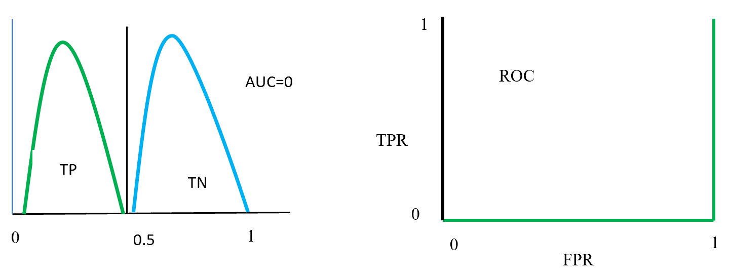
ROC distributions (class swap position distinguished)
7 Summaries
This paper describes a data mining process flow and related model and its algorithm with textual representation. One hot encoding create dummy variable for class features and min-max scaling scale the data in a single format. Balancing by SMOTE data where Euclidian distance calculates the distance in-between nearest neighbour to produce synthetic data under minority class. LDA reduce the distance inside class and maximise distance in-between class and for two class problem give a single dimension features which is less costly to calculate accuracy by base algorithm (random forest and MLP classifier). Confusion matrix gives the accuracy, precision, sensitivity, specificity which is help to take a decision about base algorithm. AUC and ROC curve also represent true positive rate against false positive rate which indicate base algorithm performance.
Base algorithm Random forest using CART with GINI impurity for feature selection to spread the tree. Here CART is selected because of less costly to run. Random forest algorithm is using bootstrap dataset to grow trees, and aggregation using majority vote to select accuracy.
MLP classifier is a neural network algorithm using backpropagation chain-rule to reducing error. Here inside layers using RLU activation function. Output layers using Sigmoid activation function and binary cross entropy loss function calculate the loss which is back propagate with Adam optimizer to optimize weight and reduce loss.
References:
- Visa, S., Ramsay, B., Ralescu, A.L. and Van Der Knaap, E., 2011. Confusion Matrix-based Feature Selection. MAICS, 710, pp.120-127.
- Grzybowski, M. and Younger, J.G., 1997. Statistical methodology: III. Receiver operating characteristic (ROC) curves. Academic Emergency Medicine, 4(8), pp.818-826.


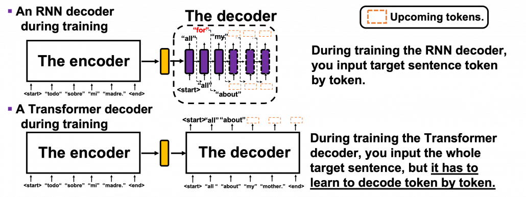
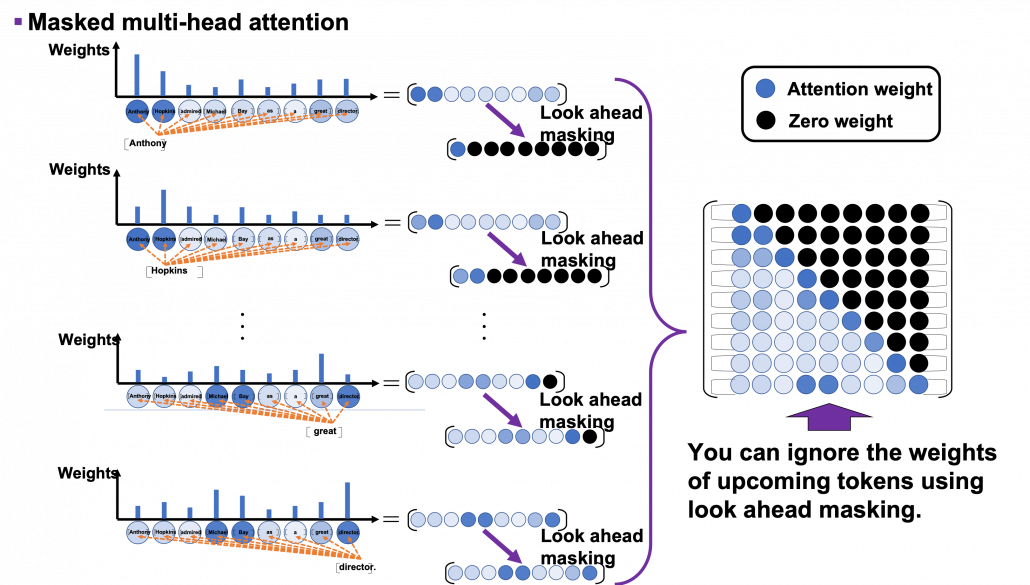
 tokens, basically you have to wait for
  the RNN cell retains the information at the time step
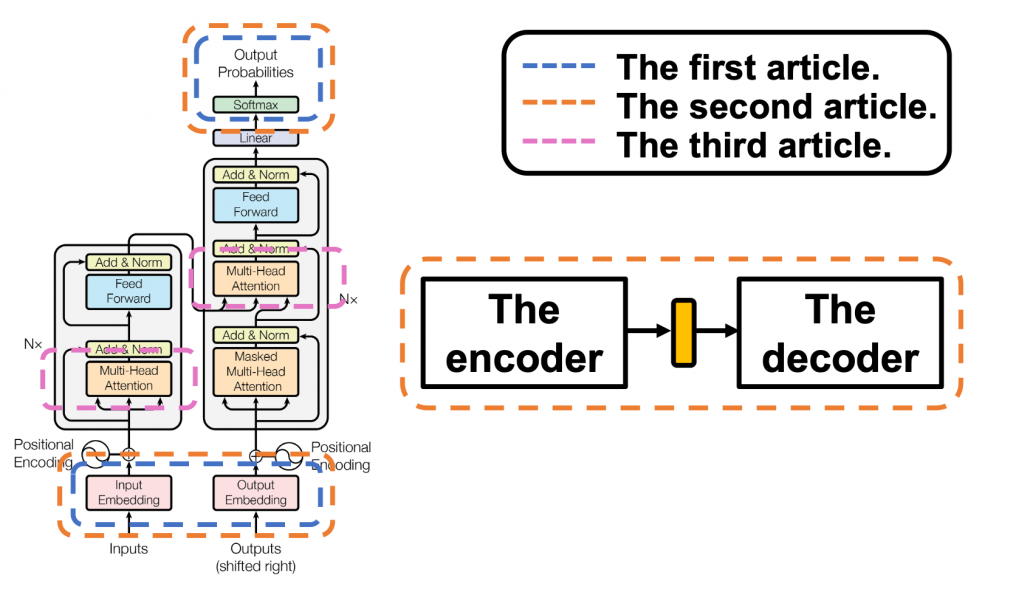
  only via recurrent connections. In this way you cannot attend to tokens in the earlier time steps, and this is obviously far from how we compare tokens in a sentence. You can bring information backward by bidirectional connection s in RNN models, but that all the more deteriorate parallelization of the model. And possessing information via recurrent connections, like a telephone game, potentially has risks of vanishing gradient problems. Gated RNN, such as LSTM or GRU mitigate the problems by a lot of nonlinear functions, but that adds to computational costs. If you understand multi-head attention mechanism, I think you can see that Transformer solves those problems.
 , but if you naively give the term
 ![[0, 1]](https://data-science-blog.com/en/wp-content/ql-cache/quicklatex.com-caffaae885a1287e3dfc31bfb1cd0694_l3.png "Rendered by QuickLaTeX.com") . With this approach, however, the resolution of encodings can vary depending on the length of the input sequence data. Thus these naive approaches do not meet the requirements above, and I guess even conventional RNN-based models were not so successful in these points.
. With this approach, however, the resolution of encodings can vary depending on the length of the input sequence data. Thus these naive approaches do not meet the requirements above, and I guess even conventional RNN-based models were not so successful in these points. ,
,  , where
  .
.  is the dimension of word embedding. The heat map below is the most typical type of visualization of positional encoding you would see everywhere, and in this case
  , and
, and  is discrete number which varies from
  to
to  , thus the heat map blow is equal to a
  matrix, whose elements are from
  to
to  . Each row of the graph corresponds to one token, and you can see that lower dimensional part is constantly changing like waves. Also it is quite easy to encode an input with this positional encoding: assume that you have a matrix of an input sentence composed of 50 tokens, each of which is a 256 dimensional vector, then all you have to do is just adding the heat map below to the matrix.
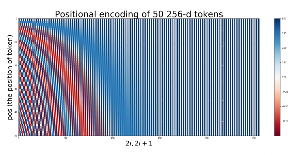

 .
. pairs of circles rather than
  , the index of the depth of each encoding, you can extract a 2 dimensional vector
 . If you constantly change the value
  rotates clockwise on the unit circle in the figure below.
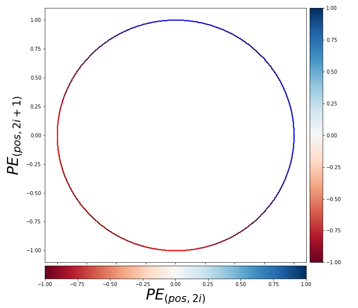
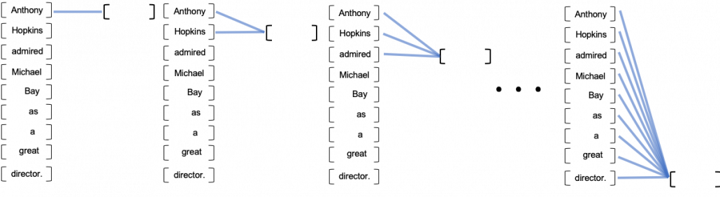
 ,
,  can be represented as a linear function of
  .” For each circle at any depth, I mean for any

 , where
  . Also the shift from “Bay” to “great” has the same rotation.
 ', fontsize=30)
plt.colorbar()
plt.title("Positional encoding of 50 256-d tokens", fontsize=40)
plt.savefig("positional_encoding_heat_map.png")
plt.show()
', fontsize=30)
plt.colorbar()
plt.title("Positional encoding of 50 256-d tokens", fontsize=40)
plt.savefig("positional_encoding_heat_map.png")
plt.show()
 ', fontsize=40)
ax.set_zlabel(r'
', fontsize=40)
ax.set_zlabel(r' ', fontsize=40)
ax.set_xticks(np.arange(0, d_model//2, 10))
plt.subplots_adjust(left=0, right=1, bottom=0, top=1)
#plt.savefig('./positional_encoding_gif/{}.png'.format(j+1))
plt.show()
', fontsize=40)
ax.set_xticks(np.arange(0, d_model//2, 10))
plt.subplots_adjust(left=0, right=1, bottom=0, top=1)
#plt.savefig('./positional_encoding_gif/{}.png'.format(j+1))
plt.show()
 , and it includes words from “a”, “ablation”, “actually” to “zombie”, “?”, “!”
 , where only the No. i element is
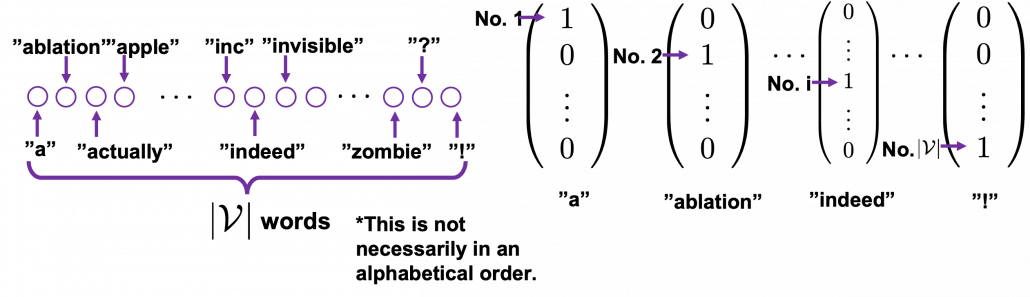
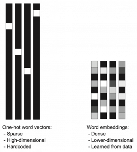
 dimensional vector, whose dimension is fewer than the vocabulary size
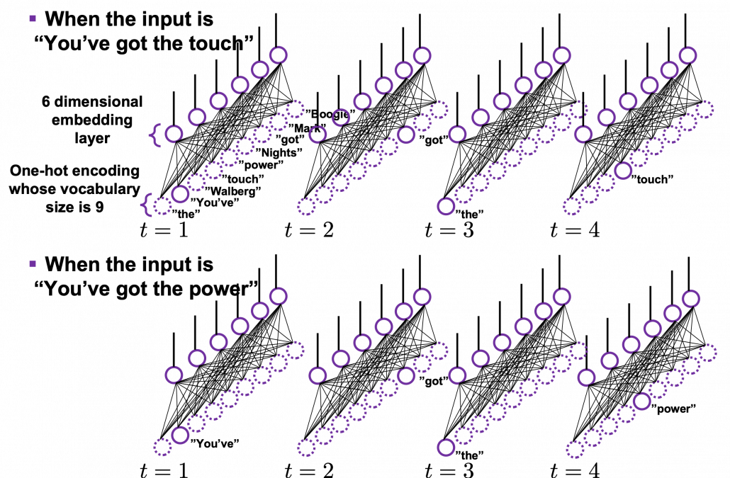
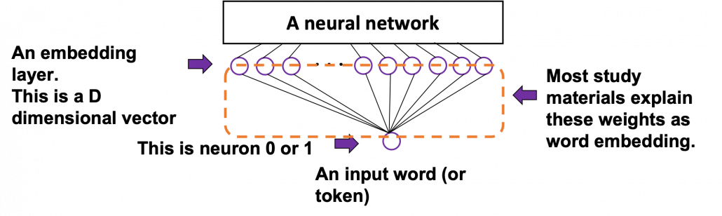
 . When the inputs are “You’ve got the touch” or “You’ve got the power” , you put the one-hot vector corresponding to “You’ve”, “got”, “the”, “touch” or “You’ve”, “got”, “the”, “power” sequentially every time step
  .
.
 ,
,  .
. , a list of vectors. The vectors are usually embedding vectors, and the
  , where
  denote “You’ve”, “got”, “the”, “power”, “.” respectively. In this case
  .
. usually includes two tokens
  and
and  at the beginning and the end of the sentence. They mean “Beginning Of Sentence” and “End Of Sentence” respectively. Thus in many cases
  .
.  and
and  are also both vectors, at least in the Tensorflow tutorial.
 is the probability of incidence of the sentence. But it is easy to imagine that it would be very hard to directly calculate how likely the sentence
  as a product of the probability of incidence or a certain word, given all the words so far. When you’ve got the words
  so far, the probability of the incidence of
  , given the context is
  .
.  is a probability of the the sentence
  , and the probability of
  can be decomposed this way:
 .
.

 .
.


 be
be  be
be ![P(\boldsymbol{x}^{(t+1)}|\boldsymbol{X}_{[0, t]})](https://data-science-blog.com/en/wp-content/ql-cache/quicklatex.com-9b85b225f0635a7627a99481018f6166_l3.png "Rendered by QuickLaTeX.com") be
be  , then
 ![P(\boldsymbol{X}) = P(\boldsymbol{x}^{(0)})\prod_{t=0}^{\tau}{P(\boldsymbol{x}^{(t+1)}|\boldsymbol{X}_{[0, t]})}](https://data-science-blog.com/en/wp-content/ql-cache/quicklatex.com-59e2d215f0fea11ec20386dfef220a30_l3.png "Rendered by QuickLaTeX.com") . Language models calculate which words to come sequentially in this way.
. Language models calculate which words to come sequentially in this way.


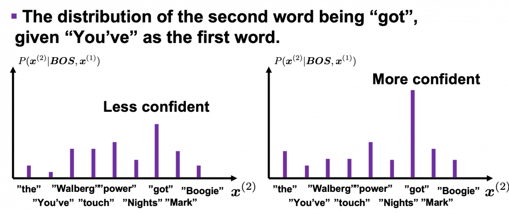
![P(\boldsymbol{x}^{(0)})\prod_{t=0}^{4}{P(\boldsymbol{x}^{(t+1)}|\boldsymbol{X}_{[0, t]})}](https://data-science-blog.com/en/wp-content/ql-cache/quicklatex.com-4d263b8554a322d3ab8a8841552bc75b_l3.png "Rendered by QuickLaTeX.com") . Given a context
. Given a context  is
is  . In the figure below, the distribution at the left side is less confident because probabilities do not spread widely, on the other hand the one at the right side is more confident that next word is “got” because the distribution concentrates on “got”.
 is
is 

 .
.


 gets higher. Thus


 gets lower, where usually
  or
or  .
. , which is composed of
  sentences in total. Each sentence
![(\boldsymbol{x}^{(0)})\prod_{t=0}^{\tau ^{(n)}}{P(\boldsymbol{x}_{n}^{(t+1)}|\boldsymbol{X}_{n, [0, t]})}](https://data-science-blog.com/en/wp-content/ql-cache/quicklatex.com-ccc74ac2aee4f90a6b035dcfd2632927_l3.png "Rendered by QuickLaTeX.com") has
has  tokens in total excluding
  . And let
  , where
 ![z = \frac{-1}{|\mathcal{V}|}\sum_{n=1}^{|\mathcal{D}|}{\sum_{t=0}^{\tau ^{(n)}}{log_{b}P(\boldsymbol{x}_{n}^{(t+1)}|\boldsymbol{X}_{n, [0, t]})}](https://data-science-blog.com/en/wp-content/ql-cache/quicklatex.com-c1ccb76fcad455ad635fc1ec8b2f6f81_l3.png "Rendered by QuickLaTeX.com") . The
. The  is usually
  or
or  .
. is vocabulary {“the”, “You’ve”, “Walberg”, “touch”, “power”, “Nights”, “got”, “Mark”, “Boogie”}. Also assume that the evaluation data set for perplexity of a language model is
  , where
 . In this case
 . I have already showed you how to calculate the perplexity of the sentence “You’ve got the touch.” above. You just need to do a similar thing on another sentence “You’ve got the power”, and then you can get the perplexity of the language model.