How Cloud Data Platforms improve Shopfloor Management
In the era of Industry 4.0, linking data from MES (Manufacturing Execution System) with that from ERP, CRM and PLM systems plays an important role in creating integrated monitoring and control of business processes.
ERP (Enterprise Resource Planning) systems contain information about finance, supplier management, human resources and other operational processes, while CRM (Customer Relationship Management) systems provide data about customer relationships, marketing and sales activities. PLM (Product Lifecycle Management) systems contain information about products, development, design and engineering.
By linking this data with the data from MES, companies can obtain a more complete picture of their business operations and thus achieve better monitoring and control of their business processes. Of central importance here are the OEE (Overall Equipment Effectiveness) KPIs that are so important in production, as well as the key figures from financial controlling, such as contribution margins. The fusion of data in a central platform enables smooth analysis to optimize processes and increase business efficiency in the world of Industry 4.0 using methods from business intelligence, process mining and data science. Companies also significantly increase their enterprise value with the linking of this data, thanks to the data and information transparency gained.
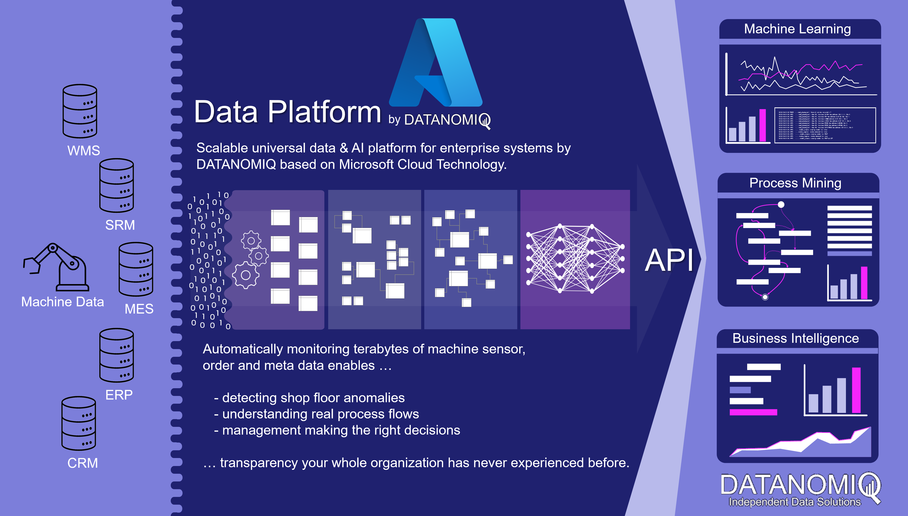
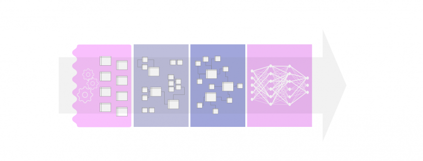
Cloud Data Platform for shopfloor management and data sources such like MES, ERP, PLM and machine data. Copyright by DATANOMIQ.
If the data sources are additionally expanded to include the machines of production and logistics, much more in-depth analyses for error detection and prevention as well as for optimizing the factory in its dynamic environment become possible. The machine sensor data can be monitored directly in real time via respective data pipelines (real-time stream analytics) or brought into an overall picture of aggregated key figures (reporting). The readers of this data are not only people, but also individual machines or entire production plants that can react to this data.
As a central data architecture there are dozens of analytical applications which can be fed with data:
– OEE key figures for Shopfloor reporting
– Process Mining (e.g. material flow analysis) for manufacturing and supply chain.
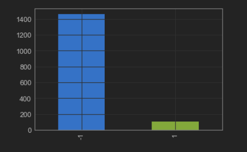
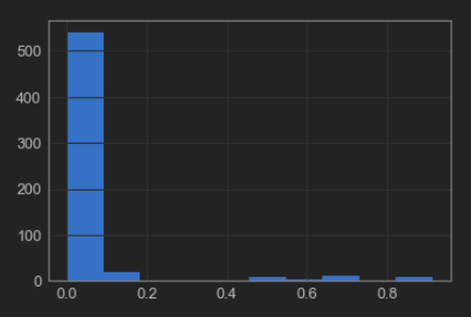
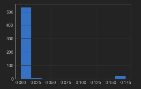
– Detection of anomalies on the shopfloor or on individual machines.
– Predictive maintenance for individual machines or entire production lines.
This solution scales completely automatically in terms of both performance and cost. It looks beyond individual problems since it offers universal and flexible scope for action. In other words, it will result in a “god mode” for the management being able to drill-down from a specific client project to insights into single machines involved into each project.
Are you interested in scalable data architectures for your shopfloor management? Or would you like to discuss a specific problem with us? Or maybe you are interested in an individual data strategy? Then get in touch with me! 🙂