Geschriebene Artikel über Big Data Analytics

Data Warehousing Basiscs

September 24, 2021/in Big Data, Business Intelligence, Data Engineering, Data Migration, Data Warehousing, Database, ETL, Graph Database, InMemory, Main Category/by Benjamin Aunkofer

Data Warehousing is applied Big Data Management and a key success factor in almost every company. Without a data warehouse, no company today can control its processes and make the right decisions on a strategic level as there would be a lack of data transparency for all decision makers. Bigger comanies even have multiple data warehouses for different purposes.

In this series of articles I would like to explain what a data warehouse actually is and how it is set up. However, I would also like to explain basic topics regarding Data Engineering and concepts about databases and data flows.

To do this, we tick off the following points step by step:

Database Concepts: ACID vs BASE
Database Concepts: CAP Theorem
Normalization of Databases (coming soon)
Data Warehouse Data Models (coming soon)
Data Lake Concepts (coming soon)

Why Do Companies Use Data Lakes?

September 15, 2021/in Data Engineering, Data Warehousing/by Philip Piletic

Modern enterprise-level computing operations have to capture a truly monumental amount of information every single hour. As the scale of data has grown almost exponentially over the years, so has the scale and complexity of data stores. Traditional databases couldn’t possibly keep up with the massive numbers of records that have to be created today, which is why so many firms ended up looking for alternatives to them.

For a while, it certainly seemed as though the new breed of data warehouses would fit the bill. Enterprises that had to harvest information from all of their inputs regarding every possible function of their businesses ran to adopt this new paradigm even as the streams of data they were collecting turned into raging rivers that some might call fire hoses. Into this scattered market entered an even new concept that attempts to refactor the data processing question into a tranquil lake as opposed to that torrential downpour.

When businesses turn to this kind of digital infrastructure, they’re often looking to make sense out of this otherwise immeasurable flood.

When Data Lakes Beat Out Warehouses

Since lakes are taking over in a space currently occupied by already existing operational structures, the data lake vs data warehouse debate is currently pretty heated. Proponents of lakes say that one of the biggest reasons that companies are turning to them is the question of vendor lock-in. When an enterprise-level user stores all of their information into a conventional warehouse, they’re locked into a single vendor who processes data on their behalf. In general, their storage and analytic algorithms are bundled together into a package that’s not easy to separate into disparate parts.

Others might be dealing with a specific processing engine that requires all of their information to be formatted a certain way as its own inputs can only understand data presented in said format. Those who’re dealing with this issue might not notice it until they finally get a flow of information that’s in some format that the warehouse engine doesn’t understand. Writing custom software to convert it isn’t an easy task, especially when there’s no API to work with.

Admittedly, these issues don’t normally come up when dealing with simple and concrete data analytics pipelines. Data warehouses do a great job of making information available and they certainly help managers draw insights from data that they might not otherwise get a chance to visualize and understand. As soon as you get into things like log analytics or processing data through machine learning technology, data warehouses will struggle. They’re normally based around relational database formats, which aren’t designed to manage semi-structured information.

Instead of going through the incredibly complex process of normalizing and cleaning all of the incoming data, it makes more sense for organization-wide IS departments to transition to a data lake.

Shifting to Data Lakes the Easy Way

Change is never easy, and that’s especially true when you’re working with IT in an enterprise market. However, the promises made by data lake proponents are attractive enough that some are making the leap. They offer an affordable single repository for all of your information regardless of what you want to store, which is why so many are now taking a dip in these virtual bodies of digital water. Structured and unstructured data can fit in together, which is certainly helping to ease the transition in many cases.

IS department staffers and technologists have found that streaming data straight from a transactional database into a data lake abstraction is a simple process. Doing so gives them the freedom to run analytics on it at a later date. Best of all, semi-structured seemingly random data points like those that come from a clickstream analysis can be moved in real-time without having to write some kind of intermediary back-end script that forces it into some kind of relational format.

However, some have taken this entirely too far and that’s where most of the criticism of data lake technology seems to be coming from. Data lakes unfortunately have to be managed carefully and the information stored in them still has to be organized in some way that makes sense and is, ideally, human readable. Locating completely unstructured data later on will simply be too difficult.

True believers in the technology have developed new solutions that get around this problem without requiring engineers to write any customized code, which has helped even skeptical businesses adopt this technology.

The Rise of Open Data Lakes

Building an open data lake is key to ensuring that any kind of processing engine can read information that comes out of the lake. That’s why an increasing number of developers are turning to platforms that don’t store this information in any proprietary format. While this might seem like it could get confusing since there are a number of different competing standards vying for market dominance, it’s actually aiding adoption.

Competition, even in the open-source community, has helped to ensure that data processing software ships with a relatively low incidence of bugs. The fact that there are multiple vendors in the space has also proven helpful to IS department heads looking to implement data lake solutions in their own organizations. Rather than just picking a single vendor who then provides everything, they could use several to handle different chores and get the best of all the available options. For instance, Amazon Athena-based technology may query information in a lake directly while IoT and log processing could be handled by something based on the Lucene library like Elasticsearch.

Some specialists might even wish to introduce Splunk or other related solutions into their custom data lake layouts. The wide variety of off-the-shelf projects has helped to dramatically reduce the number of individuals who have to write custom solutions, which makes it easy to get up and go with a new lake. Since there’s no need to convert information into a specific format, the implementation phase is usually much smoother.

Regardless of which specific solutions they elect to go with, however, it’s likely that an increasingly large percentage of the data processing market will look to data lakes. They’re quickly proving themselves to be both flexible and at least relatively easy to roll out.

Understanding the “simplicity” of reinforcement learning: comprehensive tips to take the trouble out of RL

September 11, 2021/in Artificial Intelligence, Data Science, Deep Learning, Machine Learning, Main Category/by Yasuto Tamura

*I adjusted mathematical notations in this article as close as possible to “Reinforcement Learning:An Introduction.” This book by Sutton and Barto is said to be almost mandatory for those who studying reinforcement learning. Also I tried to avoid as much mathematical notations, introducing some intuitive examples. In case any descriptions are confusing or unclear, informing me of that via posts or email would be appreciated.

Preface

First of all, I have to emphasize that I am new to reinforcement learning (RL), and my current field is object detection, to be more concrete transfer learning in object detection. Thus this article series itself is also a kind of study note for me. Reinforcement learning (RL) is often briefly compared with human trial and errors, and actually RL is based on neuroscience or psychology as well as neural networks (I am not sure about these fields though). The word “reinforcement” roughly means associating rewards with certain actions. Some experiments of RL were conducted on animals, which are widely known as Skinner box or more classically Pavlov’s Dogs. In short, you can encourage animals to do something by giving foods to them as rewards, just as many people might have done to their dogs. Before animals find linkages between certain actions and foods as rewards to those actions, they would just keep trial and errors. We can think of RL as a family of algorithms which mimics this behavior of animals trying to obtain as much reward as possible.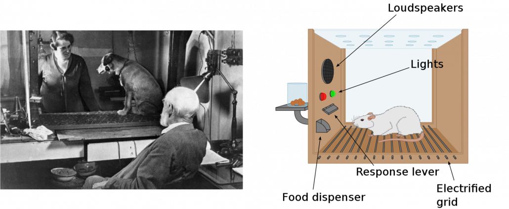

*My cats will not all the way try to entertain me to get foods though.

RL showed its conspicuous success in the field of video games, such as Atari, and defeating the world champion of Go, one of the most complicated board games. Actually RL can be applied to not only video games or board games, but also various other fields, such as business intelligence, medicine, and finance, but still I am very much fascinated by its application on video games. I am now studying the field which could bridge between the world of video games and the real world. I would like to mention this in the one of upcoming articles.

So far I got an impression that learning RL ideas would be more challenging than learning classical machine learning or deep learning for the following reasons.

RL is a field of how to train models, rather than how to design the models themselves. That means you have to consider a variety of problem settings, and you would often forget which situation you are discussing.
You need prerequisites knowledge about the models of components of RL for example neural networks, which are usually main topics in machine/deep learning textbooks.
It is confusing what can be learned through RL depending on the types of tasks.
Even after looking over at formulations of RL, it is still hard to imagine how RL enables computers to do trial and errors.

*For now I would like you to keep it in mind that basically values and policies are calculated during in during RL.

And I personally believe you should always keep the following points in your mind in order not to be at a loss in the process of learning RL.

RL basically can be only applied to a very limited type of situation, which is called Markov decision process (MDP). In MDP settings your next state depends only on your current state and action, regardless of what you have done so far.
You are ultimately interested in learning decision making rules in MDP, which are called policies.
In the first stage of learning RL, you consider surprisingly simple situations. They might be simple like mazes in kids’ picture books.
RL is in its early days of development.

Let me explain a bit more about what I meant by the third point above. I have been learning RL mainly with a very precise Japanese textbook named 「機械学習プロフェッショナルシリーズ　強化学習」(Machine Learning Professional Series: Reinforcement Learning). As I mentioned in an article of my series on RNN, I sometimes dislike Western textbooks because they tend to beat around the bush with simple examples to get to the point at a more abstract level. That is why I prefer reading books of this series in Japanese. And especially the RL one in the series was especially bulky and so abstract and overbearing to a spectacular degree. It had so many precise mathematical notations without leaving room for ambiguity, thus it took me a long time to notice that the book was merely discussing simple situations like mazes in kids’ picture books. I mean, the settings discussed were so simple that they can be expressed as tabular data, that is some Excel sheets.

*I could not notice that until the beginning of 6th chapter out of eight out of 8 chapters. The 6th chapter discusses uses of function approximators. With the approximations you can approximate tabular data. My articles will not dig this topic of approximation precisely, but the use of deep learning models, which I am going to explain someday, is a type of this approximation of RL models.

You might find that so many explanations on RL rely on examples of how to make computers navigate themselves in simple mazes or in playing video games, which are mostly impractical in the real world. However, as I will explain later, these are actually helpful examples to learn RL. As I show later, the relations of an agent and an environment are basically the same also in more complicated tasks. Reading some code or actually implementing RL would be very effective, especially in order to know simplicity of the situations in the beginning part of RL textbooks.

Given that you can do a lot of impressive and practical stuff with current deep learning libraries, you might get bored or disappointed by simple applications of RL in many textbooks. But as I mentioned above, RL is in its early days of development, at least at a public level. And in order to show its potential power, I am going to explain one of the most successful and complicated application of RL in the next article: I am planning to explain how AlphaGo or AplhaZero, RL-based AIs enabled computers to defeat the world champion of Go, one of the most complicated board games.

*RL was not used to the chess AI which defeated Kasparov in 1997. Combination of decision trees and super computers, without RL, was enough for the “simplicity” of chess. But uses of decision tree named Monte Carlo Tree Search enabled Alpha Go to read some steps ahead more effectively. It is said deep learning enabled AlphaGo to have intuition about games. Mote Carlo Tree Search enabled it to have abilities to predict some steps ahead, and RL how to learn from experience.

1. What is RL?

In conclusion I would interpret RL as follows: RL is a sub-field of training AI models, and optimal rules for decision makings in an environment are learned through RL, weakly supervised by rewards in a certain period of time. When and how to evaluate decision makings are task-specific, and they are often realized by trial-and-error-like behaviors of agents. Rules for decision makings are called policies in contexts of RL. And optimization problems of policies are called sequential decision-making problems.

You are more or less going to see what I meant by my definition throughout my article series.

*An agent in RL means an entity which makes decisions, interacting with the environment with an action. And the actions are made based on policies.

You can find various types of charts explaining relations of RL with AI, and I personally found the chart below the most plausible.

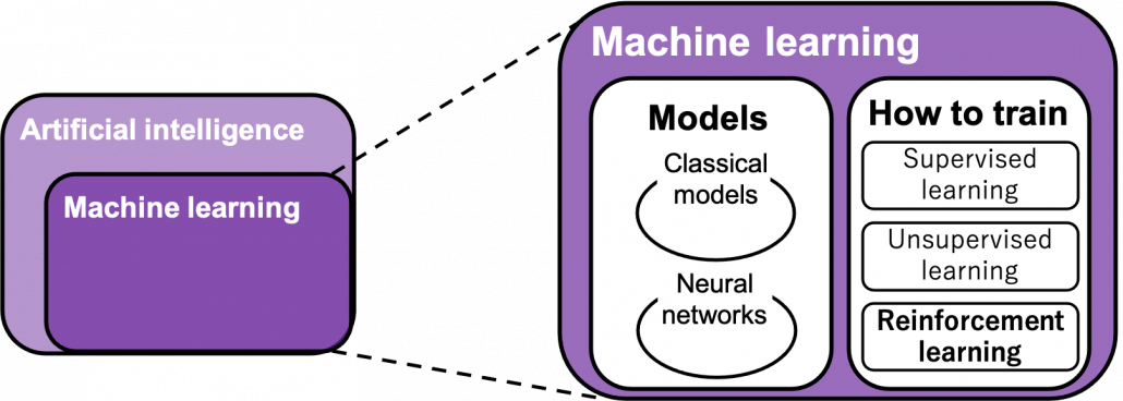“Models” in the chart are often hyped as “AI” in media today. But AI is a more comprehensive field of trying to realize human-like intellectual behaviors with computers. And machine learning have been the most central sub-field of AI last decades. Around 2006 there was a breakthrough of deep learning. Due to the breakthrough machine learning gained much better performance with deep learning models. I would say people have been calling popular “models” in each time “AI.” And importantly, RL is one field of training models, besides supervised learning and unsupervised learning, rather than a field of designing “AI” models. Some people say supervised learning or unsupervised learning are more preferable than RL because currently these trainings are more likely to be more successful in wide range of fields than RL. And usually the more data you have the more likely supervised or unsupervised learning are.

*The word “models” are used in another meaning later. Please keep it in mind that the “models” above are something like general functions. And the “models” which show up frequently later are functions modeling environments in RL.

*In case you’re totally new to AI and don’t understand what “supervising” means in these contexts, I think you should imagine cases of instructing students in schools. If a teacher just tells students “We have a Latin conjugation test next week, so you must check this section in the textbook.” to students, that’s a “supervised learning.” Students who take exams are “models.” Apt students like machine learning models would show excellent performances, but they might fail to apply the knowledge somewhere else. I mean, they might fail to properly conjugate words in unseen sentences. Next, if the students share an idea “It’s comfortable to get together with people alike.” they might be clustered to several groups. That might lead to “cool guys” or “not cool guys” group division. This is done without any explicit answers, and this corresponds to “unsupervised learning.” In this case, I would say a certain functions of the students’ brain or atmosphere there, which put similar students together, were the “models.” And finally, if teachers tell the students “Be a good student,” that’s what I meant with “weakly supervising.” However most people would say “How?” RL could correspond to such ultimate goals of education, and as well as education, you have to consider how to give rewards and how to evaluate students/agents. And “models” can vary. But such rewards often shows unexpected results.

2. RL and Markov decision process

As I mentioned in a former section, you have to keep it in mind that RL basically can be applied to a limited situation of sequential decision-making problems, which are called Markov decision processes (MDP). A markov decision process is a type of process where the next state of an agent depends only on the current state and the action taken in the current state. I would only roughly explain MDP in this article with a little formulation.

You might find MDPs very simple. But some people would find that their daily lives in fact can be described well with a MDP. The figure below is a state transition diagram of everyday routine at an office, and this is nothing but a MDP. I think many workers also basically have only four states “Chat” “Coffee” “Computer” and “Home” almost everyday. Numbers in black are possibilities of transitions at the state, and each corresponding number in orange is the reward you get when the action is taken. The diagram below shows that when you just keep using a computer, you would likely to get high rewards. On the other hand chatting with your colleagues would just continue to another term of chatting with a probability of 50%, and that undermines productivity by giving out the reward of -1. And having some coffee is very likely to lead to a chat. In practice, you optimize which action to take in each situation. You adjust probabilities at each state, that is you adjust a policy, through planning or via trial and error.

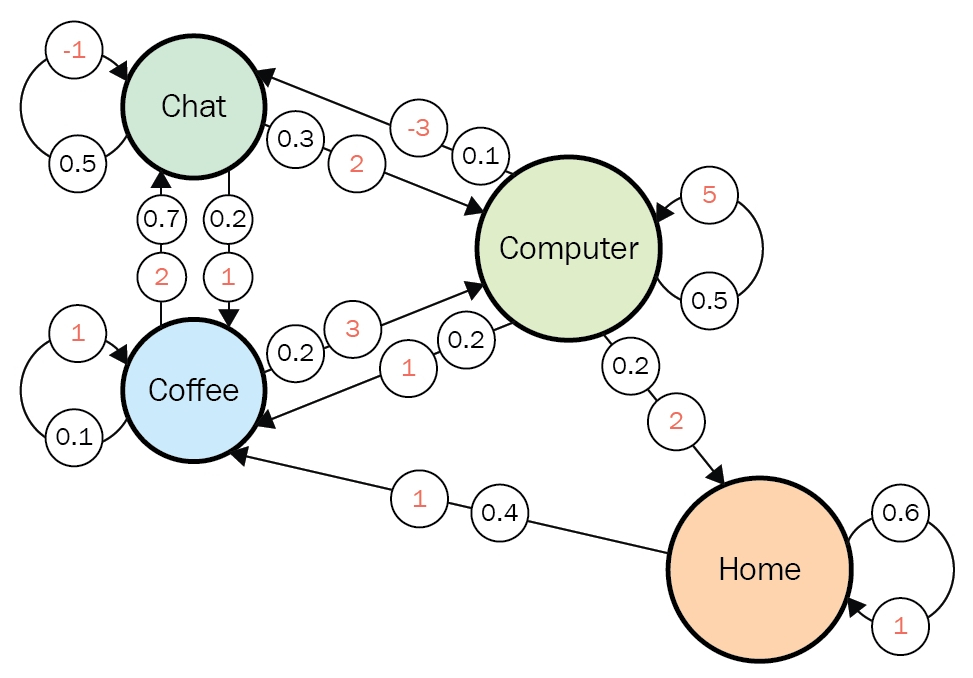
Source: https://subscription.packtpub.com/book/data/9781788834247/1/ch01lvl1sec12/markov-decision-processes

*Even if you say “Be a good student,” school kids in puberty they would act far from Markov decision process. Even though I took an example of school earlier, I am sure education should be much more complicated process which requires constant patience.

Of course you have to consider much more complicated MDPs in most RL problems, and in most cases you do not have known models like state transition diagrams. Or rather I have to say RL enables you to estimate such diagrams, which are usually called models in contexts of RL, by trial and errors. When you study RL, for the most part you will see a chart like below. I think it is important to understand what this kind of charts mean, whatever study materials on RL you consult. I said RL is basically a training method for finding optimal decision making rules called policies. And in RL settings, agents estimate such policies by taking actions in the environment. The environment determines a reward and the next state based on the current state and the current action of the agent.

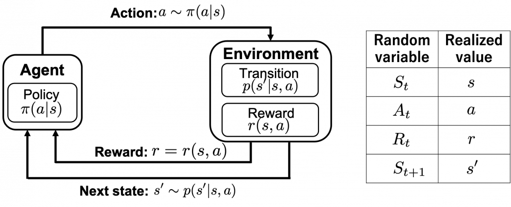
Let’s take a close look at the chart above in a bit mathematical manner. I made it based on “Machine Learning Professional Series: Reinforcement Learning.” The agent exert an action $a$ in the environment, and the agent receives a reward $r$ and the next state $s'$ . $r$ and $s'$ are consequences of taking the action $a$ in the state $s$ . The action $a$ is taken based on a conditional probability given $s$ , which is denoted as $\pi(a|s)$ . This probability function $\pi(a|s)$ is the very function representing policies, which we want to optimize in RL.

*Please do not think too much about differences of $\sim$ and $=$ in the chart. Actions, rewards, or transitions of states can be both deterministic or probabilistic. In the chart above, with the notation $a \sim \pi (a|s)$ I meant that the action $a$ is taken with a probability of $\pi (a|s)$ . And whether they are probabilistic or deterministic is task-specific. Also you should keep it in mind that all the values in the chart are realized values of random variables as I show in the chart at the right side.

In the textbook “Reinforcement Learning:An Introduction” by Richard S. Sutton, which is almost mandatory for all the RL learners, RL process is displayed as the left side of the figure below. Each capital letter in the chart means a random variable. Relations of random variables can be also displayed as graphical models like the right side of the chart. The graphical model is a time series expansion of the chart of RL loops at the left side. The chart below shows almost the same idea as the one above. Whether they use random variables or realized values is the only difference between them. My point is that decision makings are simplified in RL as the models I have explained. Even if some situations are not strictly MDPs, in many cases the problems are approximated as MDPs in practice so that RL can be applied to.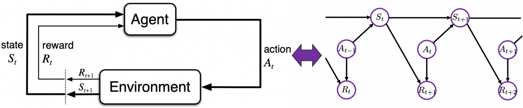

*I personally think you do not have to care so much about differences of random variables and their realized values in RL unless you discuss RL mathmematically. But if you do not know there are two types of notations, which are strictly different ideas, you might get confused while reading textboks on RL. At least in my artile series, I will strictly distinguish them only when their differences matter.

*In case you are not sure about differences of random variables and their realizations, please roughly grasp the terms as follows: random variables $X$ are probabilistic tools for example dices. On the other hand their realized values $x$ are records of them, for example (4, 1, 6, 6, 2, 1, …). And the probability that a random variable $X$ takes on the value x is denoted as $Pr\{X = x\}$ . And $X \sim p$ means the random variable $X$ is selected from distribution $p(x) \doteq \text{Pr} \{X=x\}$ . In case $X$ is a “dice,” for any $x$ $p(x) = \frac{1}{6}$ .

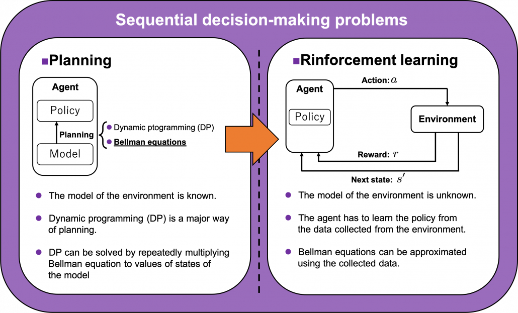
3. Planning and RL

We have seen RL is a family of training algorithms which optimizes rules for choosing $A_t = a$ in sequential decision-making problems, usually assuming them to be MDPs. However I have to emphasize that RL is not the only way to optimize such policies. In sequential decision making problems, when the model of the environment is known, policies can be optimized also through planning without collecting data from the environment. On the other hand, when the model of the environment is unknown policies have to be optimized based on data which an agents collects from the environment through trial and errors. This is the very case called RL. You might find planning problems very simple and unrealistic in practical cases. But RL is based on planning of sequential decision-making problems with MDP settings, so studying planning problems is inevitable. As far as I could see so far, RL is a family of algorithms for approximating techniques in planning problems through trial and errors in environments. To be more concrete, in the next article I am going to explain dynamic programming (DP) in RL contexts as a major example of planning problems, and a formula called the Bellman equation plays a crucial role in planning. And after that we are going to see that RL algorithms are more or less approximations of Bellman equation by agents sampling data from environments.

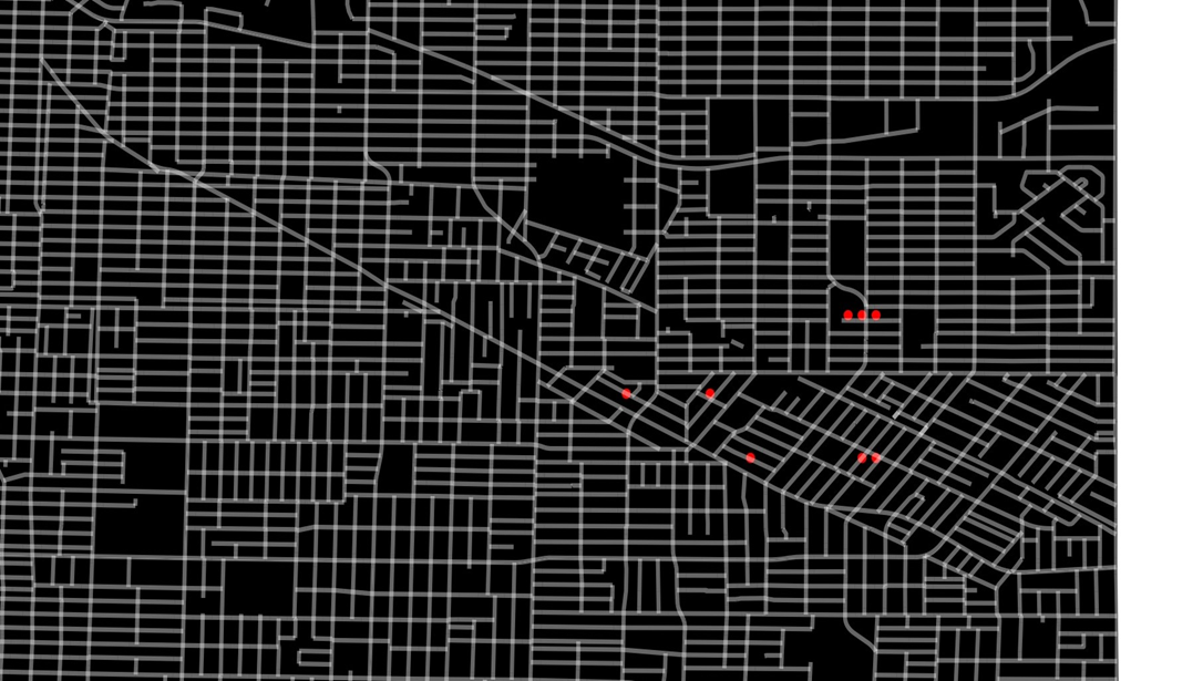
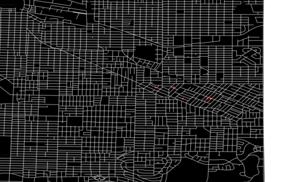
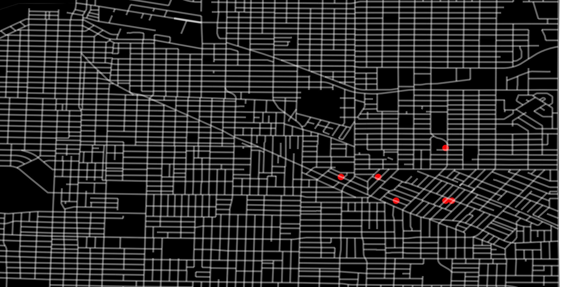
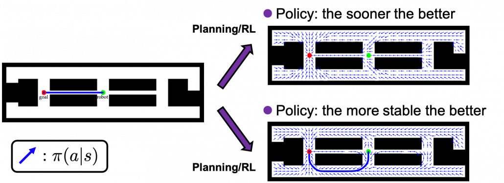
As an intuitive example, I would like to take a case of navigating a robot, which is explained in a famous textbook on robotics named “Probabilistic Robotics”. In this case, the state set $\mathcal{S}$ is the whole space on the map where the robot can move around. And the action set is $\mathcal{A} = \{\rightarrow, \searrow, \downarrow, \swarrow \leftarrow, \nwarrow, \uparrow, \nearrow \}$ . If the robot does not fail to take any actions or there are no unexpected obstacles, manipulating the robot on the map is a MDP. In this example, the robot has to be navigated from the start point as the green dot to the goal as the red dot. In this case, blue arrows can be obtained through planning or RL. Each blue arrow denotes the action taken in each place, following the estimated policy. In other words, the function $\pi$ is the flow of the blue arrows. But policies can vary even in the same problem. If you just want the robot to reach the goal as soon as possible, you might get a blue arrows in the figure at the top after planning. But that means the robot has to pass a narrow street, and it is likely to bump into the walls. If you prefer to avoid such risks, you should adopt policies of choosing wider streets, like the blue arrows in the figure at the bottom.

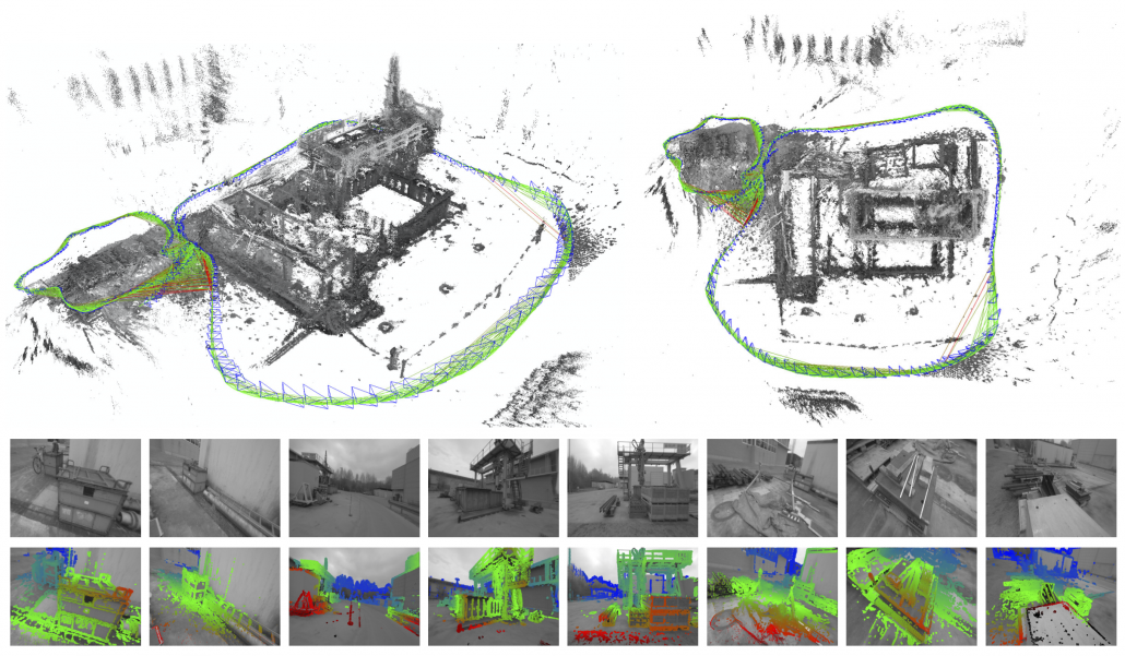
*In the textbook on probabilistic robotics, this case is classified to a planning problem rather than a RL problem because it assumes that the robot has a complete model of the environment, and RL is not introduced in the textbook. In case of robotics one major way of making a model, or rather a map is SLAM (Simultaneous Localization and Mapping). With SLAM, a map of the environment can be made only based on what have been seen with a moving camera like in the figure below. Half the first part of the textbook is about self localization of robots and gaining maps of environments. And the latter part is about planning in the gained map. RL is also based on planning problems as I explained. I would say RL is another branch of techniques to gain such models/maps and proper plans in the environment through trial and errors.

In the example of robotics above, we have not considered rewards $R_t$ in the course of navigating the agent. That means the reward is given only when it reaches the goal. But agents can get lost if they get a reward only at the goal. Thus in many cases you optimize a policy $\pi(a|s)$ such that it maximizes the sum of rewards $R_1 + R_2 + \cdots + R_T$ , where $T$ is the the length of the whole sequence of MDP in this case. More concretely, at every time step $t$ , agents have to estimate $G_t \doteq R_{t+1} + R_{t+2} + \cdots + R_T$ . The $G_t$ is called a return. But you usually have to consider uncertainty of future rewards, so in practice you multiply a discount rate $\gamma \quad (0\leq \gamma \leq 1)$ with rewards every time step. Thus in practice agents estimate a discounted return every time step as follows.

$G_t \doteq R_{t+1} + \gamma R_{t+2} + \gamma ^2 R_{t+3} + \cdots + \gamma ^ {T-t-1} R_T = \sum_{k=0}^{T-t-1}{\gamma ^{k}R_{t+k+1}}$

If agents blindly try to maximize immediate upcoming rewards $R_t$ in a greedy way, that can lead to smaller amount of rewards in the long run. Policies in RL have to be optimized so that they maximize return, a sum of upcoming rewards $G_t$ , every time step. But still, it is not realistic to take all the upcoming rewards $R_{t+1}, R_{t+2}, \dots$ directly into consideration. These rewards have to be calculated recursively and probabilistically every time step. To be exact values of states are calculated this way. The value of a state in contexts of RL mean how likely agents get higher values if they start from the state. And how to calculate values is formulated as the Bellman equation.

*If you are not sure what “ecursively” and “probabilistically” mean, please do not think too much. I am going to explain that as precisely as possible in the next article.

I am going to explain Bellman equation, or Bellman operator to be exact in the next article. For now I would like you to keep it in mind that Bellman operator calculates the value of a state by considering future actions and their following states and rewards. Bellman equation is often displayed as a decision-tree-like chart as below. I would say planning and RL are matter of repeatedly applying Bellman equation to values of states. In planning problems, the model of the environment is known. That is, all the connections of nodes of the graph at the left side of the figure below are known. On the other hand in RL, those connections are not completely known, thus they need to be estimated in certain ways by agents collecting data from the environment.

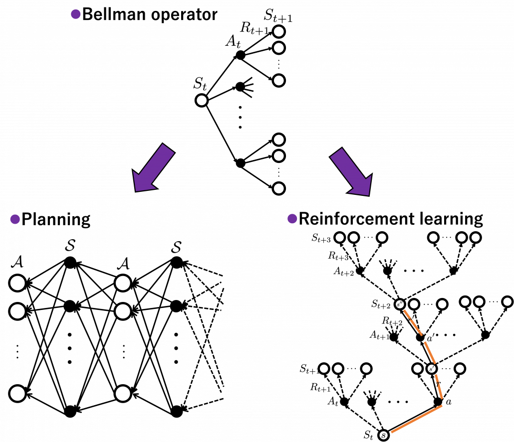
*I guess almost no one explain RL ideas as the graphs above, and actually I am in search of effective and correct ways of visualizing RL. But so far, I think the graphs above describe how values updated in RL problem settings with discrete data. You are going to see what these graphs mean little by little in upcoming articles. I am also planning to introduce Bellman operators to formulate RL so that you do not have to think about decision-tree-like graphs all the time.

4. Examples of how RL problems are modeled

You might find that so many explanations on RL rely on examples of how to make computers navigate themselves in simple mazes or play video games, which are mostly impractical in real world. But I think uses of RL in letting computers play video games are good examples when you study RL. The video game industry is one of the most developed and sophisticated area which have produced environments of RL. OpenAI provides some “playgrounds” where agents can actually move around, and there are also some ports of Atari games. I guess once you understand how RL can be modeled in those simulations, that helps to understand how other more practical tasks are implemented.

*It is a pity that there is no E.T. the Extra-Terrestrial. It is a notorious video game which put an end of the reign of Atari. And after that came the era of Nintendo Entertainment System.

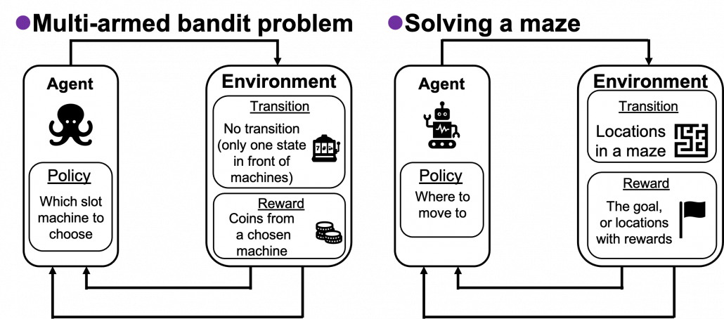
In the second section of this article, I showed the most typical diagram of the fundamental RL idea. The diagrams below show correspondences of each element of some simple RL examples to the diagram of general RL. Multi-armed bandit problems are a family of the most straightforward RL tasks, and I am going to explain it a bit more precisely later in this article. An agent solving a maze is also a very major example of RL tasks. In this case states $s\in \mathcal{S}$ are locations where an agent can move. Rewards $r \in \mathcal{R}$ are goals or bonuses the agents get in the course of the maze. 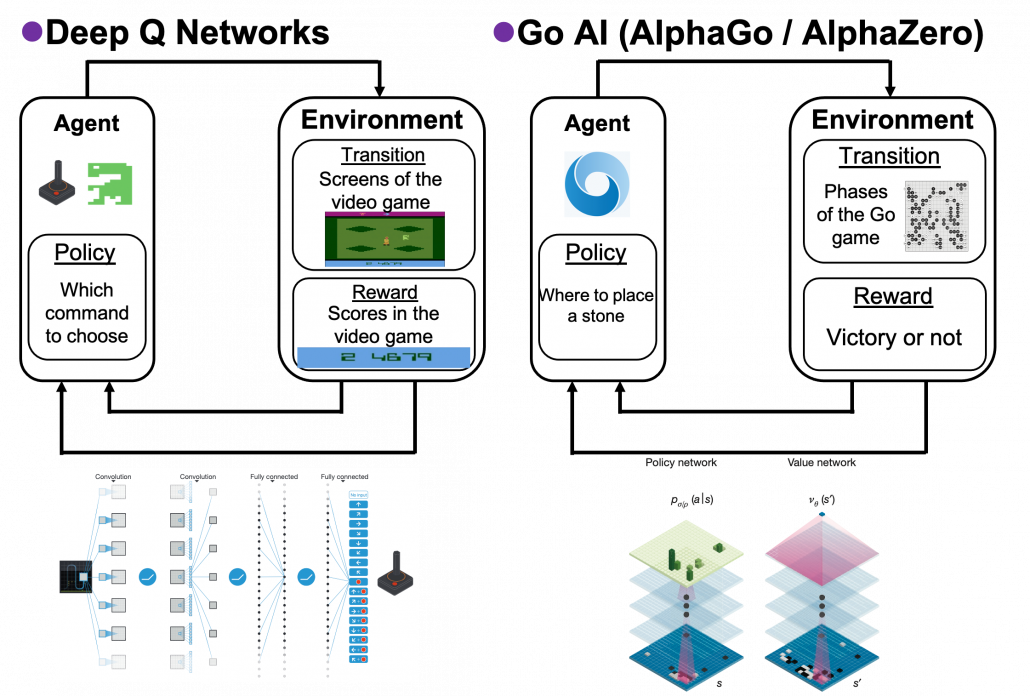And in this case $\mathcal{A} = \{\rightarrow, \downarrow,\leftarrow, \uparrow \}$ .

If the environments are more complicated, deep learning is needed to make more complicated functions to model each component of RL. Such RL is called deep reinforcement learning. The examples below are some successful cases of uses of deep RL. I think it is easy to imagine that the case of solving a maze is close to RL playing video games. In this case $\mathcal{A}$ is all the possible commands with an Atari controller like in the figure below. Deep Q Networks use deep learning in RL algorithms named Q learning. The development of convolutional neural networks (CNN) enabled computers to comprehend what are displayed on video game screens. Thanks to that, video games do not need to be simplified like mazes. Even though playing video games, especially complicated ones today, might not be strict MDPs, deep Q Networks simplifies the process of playing Atari as MDP. That is why the process playing video games can be simplified as the chart below, and this simplified MPD model can surpass human performances. AlphaGo and AlphaZero are anotehr successful cases of deep RL. AlphaGo is ther first RL model which defeated the world Go champion. And some training schemes were simplified and extented to other board games like chess in AlphaZero. Even though they were sensations in media as if they were menaces to human intelligence, they are also based on MDPs. A policy network which calculates which tactics to take to enhance probability of winning board games. But they use much more sophisticated and complicated techniques. And it is almost impossible to try training them unless you own a tech company or something with some servers mounted with some TPUs. But I am going to roughly explain how they work in one of my upcoming articles.

5. Some keywords for organizing terms of RL

As I am also going to explain in next two articles, RL algorithms are totally different frameworks of training machine learning models compared to supervised/unsupervised learnig. I think pairs of keywords below are helpful in classifying RL algorithms you are going to encounter.

(1) “Model-based” or “model-free.”

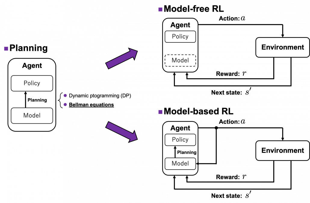
I said planning problems are basics of RL problems, and in many cases RL algorithms approximate Bellman equation or related ideas. I also said planning problems can be solved by repeatedly applying Bellman equations on states of a model of an environment. But in RL problems, models are usually unknown, and agents can only move in an environment which gives a reward or the next state to an agent. The agent can gains richer information of the environment time step by time step in RL, but this procedure can be roughly classified to two types: model-free type and model-based type. In model-free type, models of the environment are not explicitly made, and policies are updated based on data collected from the environment. On the her hand, in model-based types the models of the environment are estimated, and policies are calculated based on the model.

*AlphaGo and AlphaZero are examples of model-based RL. Phases of board games can be modeled with CNN. Plannings in this case correspond to reading some phases ahead of games, and they are enabled by Monte Carlo tree search. They are the only examples of model-based RL which I can come up with. And also I had an impression that many study materials on RL focus on model-free types of RL.

(2) “Values” or “policies.”

I mentioned that in RL, values and policies are optimized. Values are functions of a value of each state. The value here means how likely an agent gets high rewards in the future, starting from the state. Policies are functions fro calculating actions to take in each state, which I showed as each of blue arrows in the example of robotics above. But in RL, these two functions are renewed in return, and often they reach optimal functions when they converge. The figure below describes the idea well.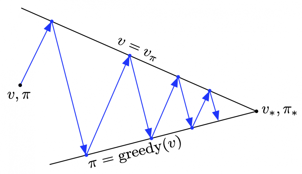

These are essential components of RL, and there too many variations of how to calculate them. For example timings of updating them, whether to update them probabilistically or deterministically. And whatever RL algorithm I talk about, how values and policies are updated will be of the best interest. Only briefly mentioning them would be just more and more confusing, so let me only briefly take examples of dynamic programming (DP).

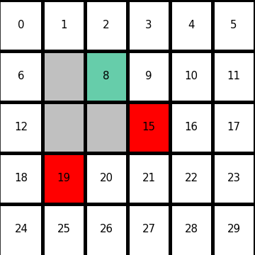
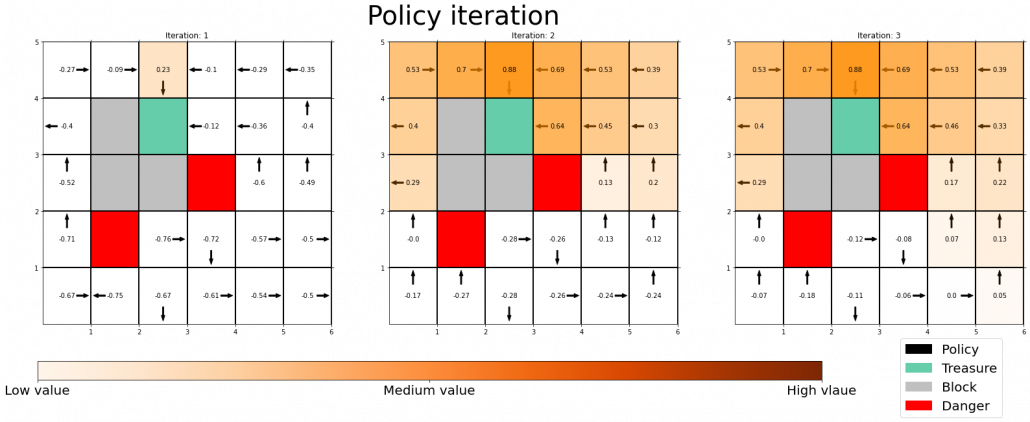
Let’s consider DP on a simple grid map which I showed in the preface. This is a planning problem, and agents have a perfect model of the map, so they do not have to actually move around there. Agents can move on any cells except for blocks, and they get a positive rewards at treasure cells, and negative rewards at danger cells. With policy iteration, the agents can interactively update policies and values of all the states of the map. The chart below shows how policies and values of cells are updated.

You do not necessarily have to calculate policies every iteration, and this case of DP is called value iteration. But as the chart below suggests, value iteration takes more time to converge.

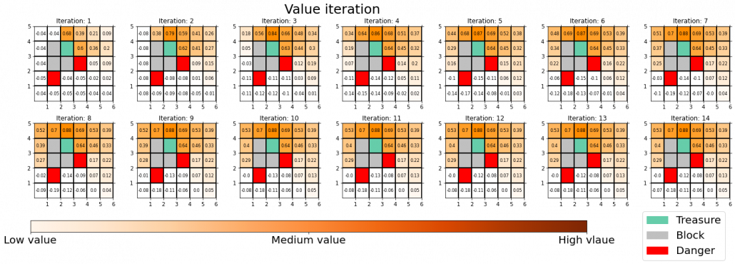
I am going to much more precisely explain the differences of values and policies in DP tasks in the next article.

(3) “Exploration” or “exploitation”

RL agents are not explicitly supervised by the correct answers of each behavior. They just receive rough signals of “good” or “bad.” One of the most typical failed cases of RL is that agents can be myopic. I mean, once agents find some actions which constantly give good reward, they tend to miss other actions which produce better rewards more effectively. One good way of avoiding this is adding some exploration, that is taking some risks to discover other actions.

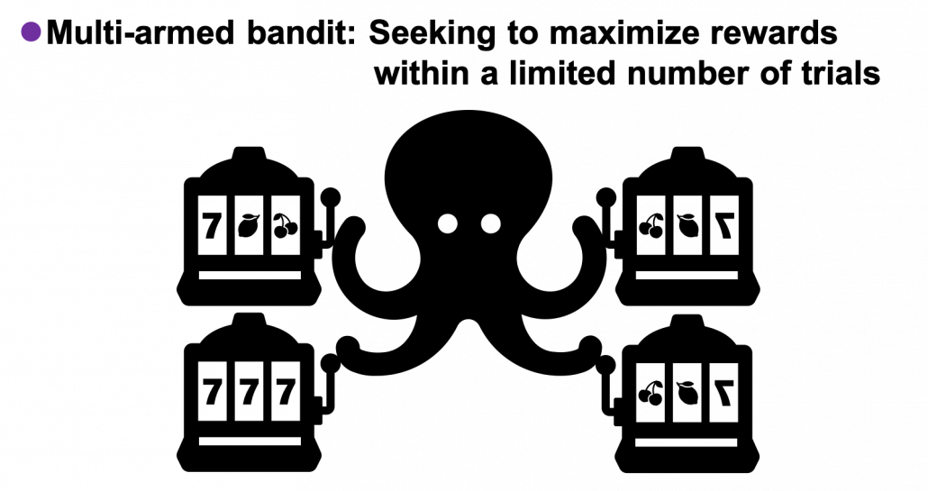
I mentioned multi-armed bandit problems are simple setting of RL problems. And they also help understand trade-off of exploration and exploitation. In a multi-armed bandit problem, an agent chooses which slot machine to run every time step. Each slot machine gives out coins, or rewards $r$ with a probability of $p$ . The number of trials is limited, so the agent has to find the machine which gives out coins the most efficiently within the limited number of trials. In this problem, the key is the balance of trying to find other effective slot machines and just trying to get as much coins as possible with the machine which for now seems to be the best. This is trade-off of “exploration” or “exploitation.” One simple way to implement exploration and exploitation trade-off is ɛ-greedy algorithm. This is quite simple: with a probability of $\epsilon$ , agents just randomly choose actions which are not thought to be the best then.

*Casino owners are not so stupid. It is designed so that you would lose in the long run, and before your “exploration” is complete, you will be “exploited.”

Let’s take a look at a simple simulation of a multi-armed bandit problem. There are two “casinos,” I mean sets of slot machines. In casino A, all the slot machines gives out the same reward $1$ , thus agents only need to find the machine which is the most likely to gives out more coins. But casino B is not simple like that. In this casino, slot machines with small odds give higher rewards.

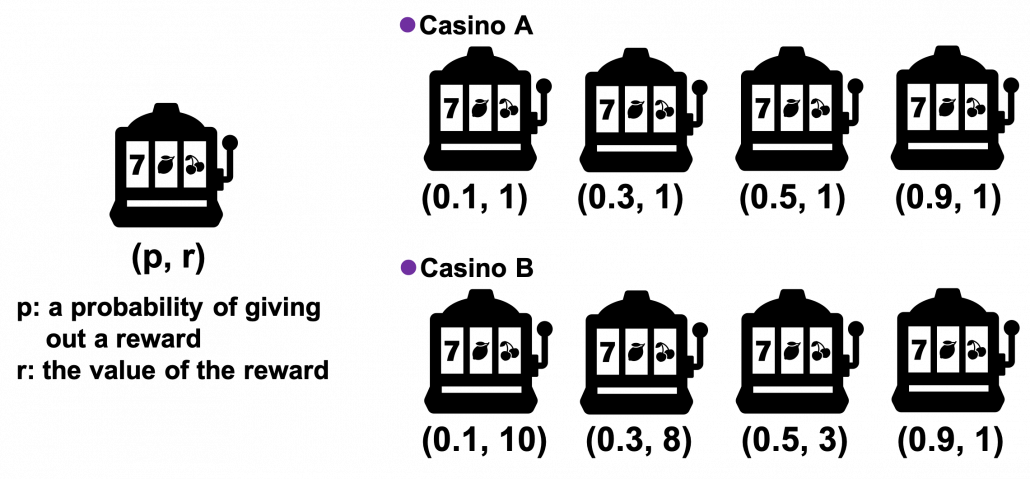
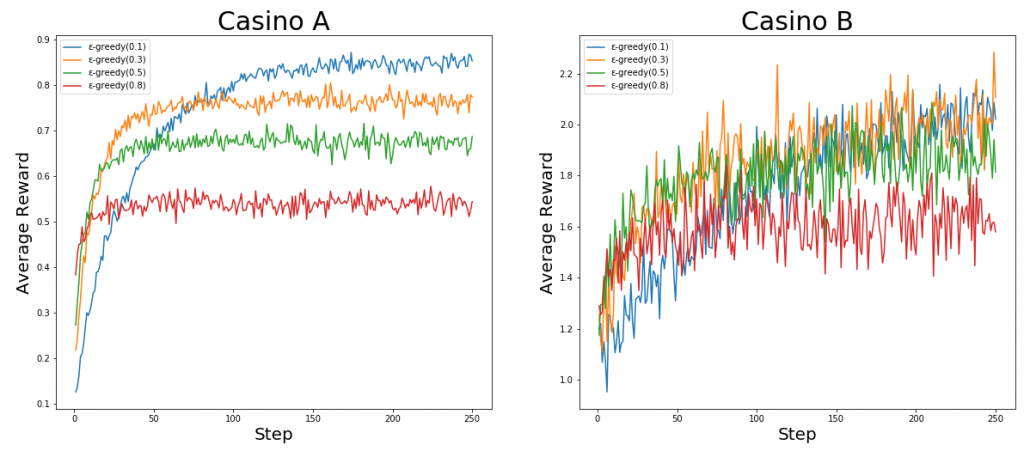
I prepared four types of “multi-armed bandits,” I mean octopus agents. Each of them has each value of $\epsilon$ , and the $\epsilon$ s reflect their “curiosity,” or maybe “how inconsistent they are.” The graphs below show the average reward over 1000 simulations. In each simulation each agent can try slot machines 250 times in total. In casino A, it seems the agent with the curiosity of $\epsilon = 0.3$ gets the best rewards in a short term. But in the long run, more stable agent whose $\epsilon$ is $0.1$ , get more rewards. On the other hand in casino B, No on seems to make outstanding results.

*I wold not concretely explain how values of each slot machines are updated in this article. I think I am going to explain multi-armed bandit problems with Monte Carlo tree search in one of upcoming articles to explain the algorithm of AlphaGo/AlphaZero.

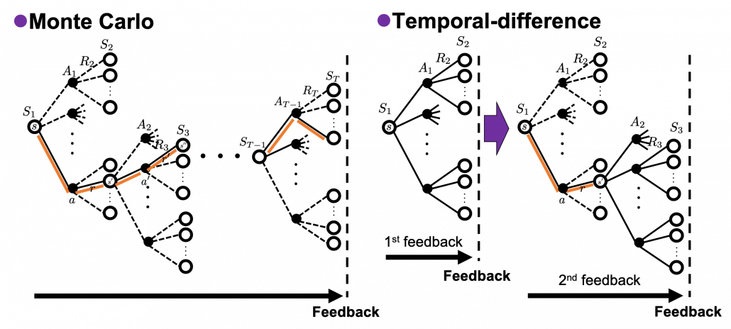
(4)”Achievement” or “estimation”

The last pair of keywords is “achievement” or “estimation,” and it might be better to instead see them as a comparison of “Monte Carlo” and “temporal-difference (TD).” I said RL algorithms often approximate Bellman equation based on data an agent has collected. Agents moving around in environments can be viewed as sampling data from the environment. Agents sample data of states, actions, and rewards. At the same time agents constantly estimate the value of each state. Thus agents can modify their estimations of values using value calculated with sampled data. This is how agents make use of their “experiences” in RL. There are several variations of when to update estimations of values, but roughly they are classified to Monte Carlo and Temporal-difference (TD). Monte Carlo is based on achievements of agents after one episode or actions. And TD is more of based on constant estimation of values at every time step. Which approach is to take depends on tasks but it seems many major algorithms adopt TD types. But I got an impression that major RL algorithms adopt TD, and also it is said evaluating actions by TD has some analogies with how brain is “reinforced.” And above all, according to the book by Sutton and Barto “If one had to identify one idea as central and novel to reinforcement learning, it would undoubtedly be temporal-difference (TD) learning.” And an intermediate idea, between Monte Carlo and TD, also can be formulated as eligibility trace.

In this article I have briefly covered all the topics I am planning to explain in this series. This article is a start of a long-term journey of studying RL also to me. Any feedback on this series, as posts or emails, would be appreciated. The next article is going to be about dynamic programming, which is a major way for solving planning problems. In contexts of RL, dynamic programming is solved by repeatedly applying Bellman equation on values of states of a model of an environment. Thus I think it is no exaggeration to say dynamic programming is the backbone of RL algorithms.

Appendix

The code I used for the multi-armed bandit simulation. Just copy and paste them on Jupyter Notebook.

* I make study materials on machine learning, sponsored by DATANOMIQ. I do my best to make my content as straightforward but as precise as possible. I include all of my reference sources. If you notice any mistakes in my materials, including grammatical errors, please let me know (email: yasuto.tamura@datanomiq.de). And if you have any advice for making my materials more understandable to learners, I would appreciate hearing it.

The Basics of Logistic Regression in Data Science

August 31, 2021/in Data Science/by Shannon Flynn

Data science is a field that is growing by leaps and bounds. A couple decades ago, using a machine learning program to make predictions about datasets was the purview of science fiction. Today, all you need is a computer, some solid programming, and a bit of patience, and you, too, can have your own digital Zoltar.

Okay, it’s not really telling the future, but it does give you the ability to predict some future events, as long as those events fall within the data the system already has. These predictions fall into two categories: linear regression and logistic regression.

Today we’re going to focus on the latter. What is logistic regression in data science, and how can it help data scientists and analysts solve problems?

What Is Logistic Regression?

First, what is logistic regression, and how does it compare to its linear counterpart?

Logistic regression is defined as “a statistical analysis method used to predict a data value based on prior observations of a data set.” It is valuable for predicting the result if it is dichotomous, meaning there are only two possible outcomes.

For example, a logistic regression system could use its data set to predict whether a specific team will win a game, based on their previous performance and the performance of their competitors because there are only two possible outcomes — a win or a loss.

Linear regression, on the other hand, is better suited for continuous output or situations where there are more than two possible outcomes. A traffic prediction model would use linear regression. In these situations, no matter how much data the program has, there are always variables that can throw a wrench in the works.

This isn’t just a case of “go” or “no go,” like you might see with a rocket launch. A company using these predictive models to schedule deliveries will need to be able to compensate for those variables. Linear regression gives them the flexibility to do that.

Logistic Regression in Data Analysis

If you broke down the expression of logistic regression on paper, it would look something like this:

The left side of the equation is called a logit, while the right side represents the odds, or the probability of success vs. failure.

It seems incredibly complicated, but when you break it down and feed it into a machine learning algorithm, it provides a great number of benefits. For one, it’s simple — in relative terms — and doesn’t generate a lot of variance because, at the end, no matter how much data you feed a logistic regression system, there are only going to be two possible outcomes.

In addition to providing you with a “yes” or “no” answer, these systems can also provide the probability for each potential outcome. The downside of logistic regression systems is that they don’t function well if you feed them too many different variables. They will also need an additional translator system to convert non-linear features to linear ones.

Applications of Logistic Regression

The potential applications for logistic regression are nearly limitless. But if you find yourself struggling to picture where you might use this data analysis tool, here are a few examples that might help you.

Organizations can use logistic regression for credit scoring. While this might seem like it’s outside the scope of this particular type of programming because there are multiple credit scores a person might have, when you break it down to ones and zeros, there are usually only two possible outcomes where credit is concerned — approved or denied.

There are a number of potential applications for logistic regression in medicine as well. When it comes to testing for a specific condition, there are usually only two results — “yes” or “no.” Either the patient has the condition, or they don’t. In this case, it may be necessary to program in a third option — a null variable — that trips when there isn’t enough information available for a particular patient to make an accurate diagnostic decision.

Even text editing can benefit from logistic regression. Plug in a dictionary, and let it loose on a piece of text. These programs aren’t going to create masterpieces or even fix editing mistakes because they lack the programming to understand things like context and tone, but they are invaluable for spelling mistakes. Again, this brings us back to the binary of 1’s and 0’s — either a word is spelled correctly, according to the dictionary definition, or it isn’t.

If dichotomous outcomes are the goal of your data analysis system, logistic regression is going to be the best tool in your toolbox.

Breaking Down the Basics

A lot goes into the creation of a machine learning or predictive analysis tool, but understanding the difference between linear and logistic regression can make that process a bit simpler. Start by understanding what the program will do, then choose your regression form appropriately.

Why Your Data Science Team Needs Separate Testing, Validation & Training Sets

August 15, 2021/in Data Science/by Philip Piletic

Automated testing of machine learning models can help to dramatically reduce the amount of time and effort that your team has to dedicate to debugging them. Not applying these techniques properly, however, could potentially do a great deal of harm if the process is completely unmonitored and doesn’t adhere to a list of best practices. Some tests can be applied to models after the training stage is over while others should be applied directly to test the assumptions that the model is operating under.

Traditionally, it’s proven somewhat difficult to test machine learning models because they’re very complex containers that often play host to a number of learned operations that can’t be clearly decoupled from the underlying software.. Conventional software can be broken up into individual units that each accomplish a specific task. The same can’t be said of ML models, which are often solely the product of training and therefore can’t be decomposed into smaller parts.

Testing and evaluating the data sets that you use for training could be the first step in unraveling this problem.

Monitoring Data Sets in a Training Environment

ML testing is very different from testing application software because anyone performing checks on ML models will find that they’re attempting to test something that is probabilistic as opposed to deterministic. An otherwise perfect model could occasionally make mistakes and still be considered the best possible model that someone could develop. Engineers working on a spreadsheet or database program wouldn’t be able to tolerate even the slightest rounding errors, but it’s at least somewhat acceptable to find the occasional flaw in the output of a program that processes data by way of learned responses. The level of variance will differ somewhat depending on the tasks that a particular model is being trained to accomplish, but it may always be there regardless.

As a result, it’s important to at least examine the initial data that’s being used to train ML models. If this data doesn’t accurately represent the kind of information that a real-world environment would thrust onto a model, then said model couldn’t ever hope to perform adequately when such input is finally given. Decent input specifications will help to ensure that the model comes away with a somewhat accurate representation of natural variability in whatever industry it’s performing a study in.

Pure performance measurements can come from essentially any test set, but data scientists will normally want to specify the hyperparameters of their model to provide a clear metric by which to judge performance while taking said measurements. Those who consistently use one model over another solely for its performance on a particular test set may end up fitting test sets to models to find something that performs exactly as they want it to.

Those who are working with smaller data sets will need to find some way to evaluate them in spite of their diminutive size.

Managing a Smaller Set of Data Safely

Those working with particularly large data sets have typically gone with 60-20-20 or 80-10-10 splits. This has helped to strike a decent balance between the competing needs of reducing potential bias while also ensuring that the simulations run fast enough to be repeated several times over.

Those working with a smaller data set might find that it simply isn’t representative enough, but for whatever reason it isn’t possible to increase the amount of information put into the test set. Cross-validation might be the best option for those who find themselves in this sort of situation. This is normally used by those in the applied ML field to compare and select models since it’s relatively easy to understand.

K-fold cross-validation algorithms are often used to estimate the skill of a particular ML model on new data irrespective of the size of the data in question. No matter what method you decide to try, though, your team needs to keep the concepts of testing and validation data separate when training your ML model. When you square these off in a training data vs. test data free-for-all, the results should come out something like this:

Test sets are essentially examples that are only ever used to judge the performance of a classifier that’s been completely specified.
Validation sets are deployed when data scientists are tuning the parameters of a classifier. You might start using a validation set to find the total number of hidden units that exist in a predefined neural network.
Training sets are used exclusively for learning. Many experts will define these as sets that are designed to fit the parameters of the initial classifier.

Segmenting testing, validation and training sets might not seem natural to those who are used to relying on one long inclusive data set in order to ensure that their ML models work in any scenario. Nevertheless, it’s vital to have them separated as much as possible. Test data management should always be part of your QA workflows. On top of this, it’s important to keep an eye on how a model responds as it learns from the data even if it does appear that accuracy increases over time. This is because there are several high-quality insights an operator can derive from the learning process.

Taking a Closer Look at Weights During the Training Process

An ideal model will enjoy lower losses and a higher degree of accuracy over time, which is often more than enough to please the data scientists that develop them. However, you can learn more by taking a close look at what areas are receiving the heaviest weights during training. A buggy piece of code could produce outcomes where different potential choices aren’t given different weights. Alternatively, it could be that they’re not really stacked against one another at all. In these cases, the overall results might end up looking realistic when they’re actually errant. Finding bugs in this way is especially important in a world where ML agents are being used to debug conventional software applications.

Taking a closer look at the weights themselves can help specialists to discover these problems before a model ever makes its way out into the wild. Debugging ML models as though they were application software will never work simply because so many aspects of their neural networks come from exclusively learned behaviors that aren’t possible to decompose into something that could be mapped on a flowchart. However, it should be possible to detect certain types of problems by paying close attention to these weights.

Developing any piece of software takes quite a bit of time, and the fact that ML models have to be trained means that they’ll often take even longer. Give yourself enough lead time and you should find that your testing, validation and training sets split evenly into different neat packages that make the process much simpler.

My elaborate study notes on reinforcement learning

July 31, 2021/in Artificial Intelligence, Data Science, Data Science Hack, Deep Learning, Machine Learning, Main Category, Use Cases/by Yasuto Tamura

I will not tell you why, but all of a sudden I was in need of writing an article series on Reinforcement Learning. Though I am also a beginner in reinforcement learning field. Everything I knew was what I learned from one online lecture conducted in a lazy tone in my college. However in the process of learning reinforcement learning, I found a line which could connect the two dots, one is reinforcement learning and the other is my studying field. That is why I made up my mind to make an article series on reinforcement learning seriously.

To be a bit more concrete, I imagine that technologies in our world could be enhanced by a combination of reinforcement learning and virtual reality. That means companies like Toyota or VW might come to invest on visual effect or video game companies more seriously in the future. And I have been actually struggling with how to train deep learning with cgi, which might bridge the virtual world and the real world.

As I am also a beginner in reinforcement learning, this article series would a kind of study note for me. But as I have been doing in my former articles, I prefer exhaustive but intuitive explanations on AI algorithms, thus I will do my best to make my series as instructive and effective as existing tutorial on reinforcement learning.

This article is going to be composed of the following contents.

Understanding the “simplicity” of reinforcement learning: comprehensive tips to take the trouble out of RL
Graphical understanding of dynamic programming and the Bellman equation: taking a typical approach at first
Four essential ideas for making reinforcement learning and dynamic programming more effective
How computers “experience” things: model-free reinforcement learning and temporal difference
A thaw in another winter of artificial intelligence: uses of deep learning in reinforcement learning (coming soon!)

In this article I would like to share what I have learned about RL, and I hope you could get some hints of learning this fascinating field. In case you have any comments or advice on my “study note,” leaving a comment or contacting me via email would be appreciated.

How to Successfully Perform a Data Quality Assessment (DQA)

July 17, 2021/in Business Analytics, Data Migration, Data Warehousing/by Shannon Flynn

People generate 2.5 quintillion bytes of data every single day. That’s 1.7 megabytes generated every second for each of the 7.8 billion residents of Earth. A lot of that information is junk that somebody can easily discard, but just as much can prove to be vital. How do you tell the difference?

According to industry experts, poor quality information costs the U.S. economy upwards of $3.1 trillion annually. That is why data quality assessments (DQAs) are so important.

A Brief Explanation of Data Quality Assessments

With companies around the globe generating massive amounts of data every second of the day, it’s essential to have tools that help you sort through it all. Data quality assessments are usually carried out by software programmed with a predefined set of rules. They can compare the incoming information to those guidelines and provide reports.

This is a simplified explanation, but the goal of these DQA programs is to separate the wheat from the chaff. They eliminate any unnecessary or redundant data, leaving only the highest quality information.

The biggest challenge here is figuring who will determine what is considered quality. Data quality depends on three things: the individual or team that creates the requirements, how they complete that task, and how flexible the program meets those obligations.

How to Perform a DQA

Once you have your DQA program in place, performing an assessment is relatively simple. The challenge lies in establishing the program. The first step is to determine the scope of the data you’re trying to assess. The details of this step will depend on your system and the amount of information you have to sort through. You can set up a program to assess a single data point at a time, but if your system generates a lot of info, this isn’t effective from an efficiency standpoint.

Define your scope carefully to ensure the program does the job correctly without wasting time sorting through bytes one at a time.

Now that you have a framework to work from, you can move on to monitoring and cleansing data. Analyze your information against the scope and details you’ve established. Validate each point against your existing statistical measures, and determine its quality.

Next, ensure all the data requirements are available and correctly formatted. You may wish to provide training for any new team members entering information to ensure it’s in a format that the DQA system can understand.

Finally, make it a point to verify that your data is consistent with the rules you’ve established, as well as your business goals. DQAs aren’t a one-and-done kind of program. Monitoring needs to be an ongoing process to prevent things from falling through the cracks and keeping bad information from potentially costing you millions of dollars.

Benefits of DQA

A data quality assessment has various benefits, both on the commercial and consumer side of your business. Accuracy is essential. It’s valuable for marketers who purchase demographic data, with 84% stating it plays a large role in their purchase decisions. Targeted marketing is one of the most popular forms of advertisement, and while it’s not always practical, its efficacy drops even further if the demographic data is incorrect.

High-quality data should be accurate, complete, relevant, valid, timely and consistent. Maintaining frequent and comprehensive quality assessments can help you do that and more. The goal of collecting this information is to produce results. The higher quality your data is, the easier and faster your system will work, with better results than you might manage without DQAs.

Data Quality Assessment vs. Data Profiling

When talking about data quality, you’ll often see the terms assessment and profiling used interchangeably. While the concepts are similar, they are not the same. Data profiling is a valuable tool for setting up your quality assessment program, giving you the information you’ll need to build your program in the future. It isn’t a step you can perform independently and expect to get the same results.

If you don’t already have a DQA in place, start with profiling to create the foundation for a comprehensive data quality assessment program.

The Growing Importance of Data Quality

Data quality has always been important. However, as the population generates more information every year, learning how to separate value from junk is more critical than ever.

Coffee Shop Location Predictor

July 12, 2021/in Data Mining, Data Science, Data Science Hack, Main Category, Predictive Analytics, Python, Tutorial, Visualization/by Mrinalini Sunder

As part of this article, we will explore the main steps involved in predicting the best location for a coffee shop in Vancouver. We will also take into consideration that the coffee shop is near a transit station, and has no Starbucks near it. Well, while at it, let us also add an extra feature where we make sure the crime in the area is lower.

Introduction

In this article, we will highlight the main steps involved to predict a location for a coffee shop in Vancouver. We also want to make sure that the coffee shop is near a transit station, and has no Starbucks near it. As an added feature, we will make sure that the crime concentration in the area is low, and the entire program should be implemented in Python. So let’s walk through the steps.

Steps Required

Get crime history for the last two years
Get locations of all transit stations and Starbucks in Vancouver
Check all the transit stations that do not have any Starbucks near them
Get all the data regarding crimes near the filtered transit stations
Create a grid of all possible coordinates around the transit station
Check crime around each created coordinate and display the top 5 locations.

Gathering Data

This covers the first two steps required to get data from the internet, both manually and automatically.

Getting all Crime History

We can get crime history for the past 14 years in Vancouver from here. This data is in raw crime.csv format, so we have to process it and filter out useless data. We then write this processed information on the crime_processed.csv file.

Note: There are 530,653 records of crime in this file

In this program, we will just use the type and coordinate of the crime. There are many crime types, but we have classified them into three major categories namely;

Theft (red), Break and Enter (orange) and Mischief (green)

These all crimes can be plotted on Graph as displayed below.

This may seem very congested and full, so let’s see a closeup image for future references.

Getting Locations of all Rapid Transit Stations

We can get the coordinates of all Transit Stations in Vancouver from here. This dataset has all coordinates of rapid transit stations in three transit lines in Vancouver. There are a total of 23 of them in Vancouver, we can then use it for further processing.

Getting Locations of all Starbucks

The Starbucks data is present here, we can scrape it easily and get the locations of all the Starbucks in Vancouver. We just need the Starbucks that is near transit stations, so we’ll filter out the rest. There are a total 24 Starbucks in Vancouver, and 10 of them are near Transit Stations.

Note: Other than the coordinates of Transit Stations and Starbucks, we also need coordinates and type of the crime.

Transit Stations with no Starbucks

As we have all the data required, now moving to the next step. We need to get to the transit Station locations that have no Starbucks near them. For that we can create an area of particular radius around each Transit Station. Then check all Starbucks locations with respect to them, whether they are within that area or not.

If none of the Starbucks are within that particular Transit Station’s area, we can append it to a list. At the end, we have a list of all Transit locations with no Starbucks near them. There are a total of 6 Transit Stations with no Starbucks near them.

Crime near Transit Stations

Now lets filter out all crime records and get just what we are interested in, which means the crime near Transit stations. For that we will plot an area of specific radius around each of them to see the crimes. These are more than 110,000 crime records.

Crime near located Transit Stations

Now that we have all the Transit Stations that don’t have any Starbucks near them and also the crime near all Transit Stations. So, let’s use this information and get crime near the located Transit Stations. These are about 44,000 crime records.

This may seem correct at first glance, but the points are overlapping due to abundance, so we can create different lists of crimes based on their types.

Theft

Break and Enter

Mischief

Generating all possible coordinates

Now finally, we have all the prerequisites and let’s get to the main task at hand, predicting the best coordinate for the coffee shop.

There may be many approaches to solve this problem, but the one I used in this program is that I will create a grid of all possible locations (coordinates) in the area of 1 km radius around each located transit station.

Initially I generated 1 coordinate for every m, this resulted in 1000,000 coordinates in every km. This is a huge number, and for the 6 located Transit stations, it becomes 6 Million. It may not seem much at first glance because computers can handle such data in a few seconds.

But for location prediction we need to compare each coordinate with crime coordinates. As the algorithm has to check for ~7,000 Thefts, ~19,000 Break ins, and ~17,000 Mischiefs around each generated coordinate. Computing this would want the program to process an estimate of 432.4 Billion times. This sort of execution takes many hours on normal computers (sometimes days).

The solution to this is to create a coordinate for each 10 m area, this results about 10,000 coordinate per km. For the above mentioned number of crimes, the estimated processes will be several Billions. That would significantly reduce the time, but is still not less.

To control this, we can remove the duplicate values in crime coordinates and those which are too close to each other ~1m. Doing so, we are left with just 816 Thefts, 2,654 Break ins, and 8,234 Mischiefs around each generated coordinate.
The precision will not be affected much but the time and computational resources required will be reduced a lot.

Checking Crime near Generated coordinates

Now that we have all the locations, we will start some processing on it and check each coordinate against some constraints. That are respectively;

Filter out Coordinates having Theft near 1 km
We get 122,000 coordinates with no Thefts (Below merged 1000 to 1)
Filter out Coordinates having Break Ins near 200m
We get 8000 coordinates with no Thefts (Below merged 1000 to 1)
Filter out Coordinates having Mischief near 200m
We get 6000 coordinates with no Thefts (Below merged 1000 to 1)
Now that we have 6 Coordinates of best locations that have passed through all the constraints, we will order them.To order them, we will check their distance from the nearest transit location. The nearest will be on top of the list as the best possible location, then the second and so on. The generated List is;
1. -123.0419406741792, 49.24824259252004
2. -123.05887151659479, 49.24327221040713
3. -123.05287151659476, 49.24327221040713
4. -123.04994067417924, 49.239242592520064
5. -123.0419406741792, 49.239242592520064
6. -123.0409406741792, 49.239242592520064

How can MindTrades help?

MindTrades Consulting Services, a leading marketing agency provides in-depth analysis and insights for the global IT sector including leading data integration brands such as Diyotta. From Cloud Migration, Big Data, Digital Transformation, Agile Deliver, Cyber Security, to Analytics- Mind trades provides published breakthrough ideas, and prompt content delivery. For more information, refer to mindtrades.com.

Code

https://github.com/Mindtrades-Consulting/Coffee-Shop-Location-Predictor

What Is Data Lake Architecture?

June 24, 2021/in Data Engineering, Data Warehousing/by Shannon Flynn

The volume of information produced by everyone in the world is growing exponentially. To put it in perspective, it’s estimated that by 2023 the big data analytics market will reach $103 billion.

Finding probable solutions for storing big data is a challenge. It’s no easy task to hold enormous amounts of information, clean it and transform it into understandable subsets — it’s best to take one step at a time.

Some reasons why companies access their big data is to:

Improve their consumer experience
Draw conclusions and make data-driven decisions
Identify potential problems
Create innovative products

There are ways to help define big data. Combining its characteristics with storage management methods help experts make their clients’ information digestible and understandable. Cue data lakes, which are repositories for big data in its native form.

Think of an actual lake with multiple water sources around the perimeter flowing into it. Picture these as three types of data: structured, semi-structured and unstructured. All this information can remain in a data lake and be accessed in its raw form at any time, making it an attractive storage method.

Here’s how data lakes are created, some of their components and how to avoid common pitfalls.

Creating a Data Lake

One benefit of creating and implementing a data lake is that structuring becomes much more manageable. Pulling necessary information from a lake allows analysts to compare and contrast data and communicate any connections between datasets to their client.

There are four steps to follow when setting up a data lake:

Choosing a software solution: Microsoft, Amazon and Google are cloud vendors that allow developers to create data lakes without using servers.
Identifying where data is sourced: Where is your information coming from? Once sources are identified, determine how your data will be cleaned or transformed.
Defining process and automation: It’s vital to outline how information should be processed once the data lake ingests it. This creates consistency for businesses.
Establishing retrieval governance: Choosing who has access to what types of information is crucial for companies with multiple locations and departments. It helps with overall organization. Data scientists, for this reason, primarily access data lakes.

The next step would be to determine the extract, transform and load (ETL) process. ETL creates visual interpretations of data to provide context to businesses. When information from a data lake is sent to a warehouse, it can be analyzed.

Components of a Data Lake

Here is what happens to information once a data lake is created:

Collection: Data comes in from various sources.
Ingestion: Data is processed using management software.
Blending: Data is combined from multiple sources.
Transformation: Data is analyzed and made sense of.
Publication: Data can be used to drive business decisions.

There are other aspects of a data lake to keep in mind. These are the critical components that help provide business solutions:

Security: Data lakes require security to protect information — they do not have built-in safety measures.
Governance: Determine who can check on the quality of data and perform measurements.
Metadata: This provides information about other data to improve understanding.
Stewardship: Choose one or more employees to take on the responsibility of managing data.
Monitoring: Employ other software to perform the ETL process.

Big data lends itself to incorporating multiple processes to make it usable for companies. The volume of information one company produces is massive — to manage it, experts need to consider these components and steps when building a data lake.

What to Avoid When Using Data Lakes

The last thing people want for their data lake is to see it turn into a swamp. When big data is processed incorrectly, its value decreases, making it useless to the business sourcing it.

The first step in avoiding a common pitfall is to consider the sustainability of the data lake. Planning processes are necessary to ensure it’s secure, and governing and regulating incoming information will allow for long-term use.

A lack of security causes another problem that can arise in data lakes. Safety measures must be implemented. Because enterprises will build data lakes for different purposes, it’s easy for information to become unorganized and vulnerable to hacking. With security, the likelihood of data breaches decreases, and the quality of data remains high.

The most important thing to remember about data lakes is the planning stage. Without proper preparation, they tend to be overwhelming due to their size and complexity. Taking the time and care to establish the processes ahead of time is vital.

Using Data Lake Architecture for Business

Data lakes store massive amounts of information to be used later on to create subsets, analyze metadata and more. Their advantages allow businesses to be flexible, save money and have access to raw information at all times.

How Microsoft Azure Is Impacting Financial Companies

June 16, 2021/in Cloud, Insights, Use Cases/by Renata Kalsbeek

Microsoft Azure has taken a large chunk of the cloud marketplace, transforming companies with the speed and security of the cloud. Microsoft has over the years used Azure to cushion companies against risk, deal with fraud and differentiate their customer experience.

With Microsoft Cloud App Security, customers experience 75% automatic threat elimination because of increased visibility and automated threat protection. With all these and more amazing benefits of using Azure, its market share is bound to increase even more over the coming years.

Image Source

Financial companies have not been left behind by the Azure bandwagon. The financial industry is using Microsoft Azure to enhance its core functions— invest money by making informed decisions, and minimize risk while maximizing returns.

Azure facilitates these core functions by helping with the storage of huge amounts of data— some dating back to decades ago—, data retrieval and data security.

It also helps financial companies to keep up with regulatory compliance.

Microsoft Azure is not the only cloud services provider. But here’s why it is the most outstanding when it comes to helping financial companies achieve their business goals.

Azure Offers Hybrid and Multi-Cloud Computing for Financial Companies

The financial services industry is extremely dynamic. Organizations offering financial services have to constantly test the market and come up with new and innovative products and services.

They are also often under pressure to extend their services across borders. Remember they have to do all of this while at the same time managing their existing customers, containing their risk, and dealing with fraud.

Financial regulations also keep changing. As financial companies increasingly embrace new technology for their services— including intelligent cloud computing— and they have to comply with industry regulations. They cannot afford to leave loopholes as they take on their journey with the cloud.

The financial services industry is highly competitive and keeps up with modernity. These companies have had to resort to the dynamic hybrid, multi-cloud computing, and public cloud strategies to keep up with the trend.

This is how a hybrid cloud model works— it enables existing on-premises applications to be extended through a connection to the public cloud.

This allows financial companies to enjoy the speed, elasticity, and scale of the public cloud without necessarily having to remodel their entire applications. These organizations are afforded the flexibility of deciding what parts of their application remains in an existing data center and which one resides in the cloud.

Cloud computing with Azure allows financial organizations to operate more efficiently by providing end-to-end protection to information, allowing the digitization of financial services, and providing data security.

Data security is particularly important to financial firms because they are often targeted by fraudsters and cyber threats. They, therefore, need to protect crucial information which they achieve by authenticating their data centers using Azure.

Here’s why financial companies cannot think of doing without Azure’s hybrid cloud computing even for just a day.

Photo by Windows on Unsplash

The ability to expand their geographic reach

Azure enables financial companies to establish data centers in new locations to meet globally growing demand. This allows them to open and explore new markets. They can then use Azure DevOps pipelines to maintain their data factories and keep everything consistent.

Consistent Infrastructure management

The hybrid cloud model promotes a consistent approach to infrastructure management across all locations, whether it is on-premises, public cloud, or the edge.

Increased Elasticity

Financial firms and banks utilizing Azure services can respond with great agility to transactional changes or changes in demand by provisioning or de-provisioning as the situation at hand demands.

In cases where the organization requires high computation such as complex risk modeling, a hybrid strategy allows it to expand its capacity beyond its data center without overwhelming its servers.

Flexibility

A hybrid strategy allows financial organizations to choose cloud services that fall within their budget, match their needs, and suit their features.

Data security and enhanced regulatory compliance

Hybrid and multi-cloud strategies are a superb alternative for strictly on-premises strategies when one considers resiliency, data portability, and data security.

Reduces CapEx Expenses

Managing on-premises infrastructure is expensive. Financial companies utilizing Azure do not need to spend large amounts of money setting them up and managing them.

With the increased elasticity of the hybrid system, financial organizations only pay for the resources they actually use, at a relatively lower cost.

Financial Organizations Have Access to an Analytics Platform

As we mentioned earlier, financial companies have the core function of making financial decisions in order to invest money and gain maximum returns at the least possible risk.

Having been entrusted with their customers’ assets, the best way to ensure success in making profits is by using an analytics system.

Getting the form of analytics that helps with solving this investment problem is the kind of headache that does not go away by taking a tablet of ibuprofen and a glass of water— integrating data is not an easy task. Besides, building a custom analytics solution from scratch is quite expensive.

Luckily for financial companies, Azure has a dedicated analytics platform for the financial services industry. It is custom-made just for these types of organizations.

Their system is quite intuitive and easy to use. Companies not only get to save the resources they would have otherwise used to build a custom solution, but they get to learn about their investment risks and get instant results at cloud speed.

They can mitigate against negatively impactful market occurrences and gain profits even when operating in adverse market conditions.

Image by Headway on Unsplash

Financial Companies Get Advanced Data Management

Good analytics goes hand-in-hand with a great data management system. Financial companies need to have good data, create an organized data warehouse, and have a secure data storage system.

In addition to storing your data, Microsoft Azure ensures your storage can be optimized to support advanced applications, for example, machine learning and forecasting.

Azure even allows you to compress and store documents for long periods of time when you write the data to Microsoft Azure Blob Storage. These documents can be retrieved anytime when the need arises for auditors’, regulators’, and lawyers’ perusal.

Conclusion

Microsoft has over time managed to gain the trust of many industries, the financial services industry inclusive. Using its cloud computing giant, Azure, it has empowered these companies to carry out their functions efficiently and at the lowest cost and risk possible.

Azure’s hybrid cloud computing strategy has made financial operations flexible, opened doors for financial companies to establish their services in multiple locations, and provided them with consistent infrastructure management, among many other benefits.

With their futuristic model and commitment to growth, it’s only prudent to assume that Microsoft Azure will continue carrying the mantle as the best cloud services provider in the financial services industry.