Geschriebene Artikel über Big Data Analytics

Language Detecting with sklearn by determining Letter Frequencies

Of course, there are better and more efficient methods to detect the language of a given text than counting its lettes. On the other hand this is a interesting little example to show the impressing ability of todays machine learning algorithms to detect hidden patterns in a given set of data.

For example take the sentence:

“Ceci est une phrase française.”

It’s not to hard to figure out that this sentence is french. But the (lowercase) letters of the same sentence in a random order look like this:

“eeasrsçneticuaicfhenrpaes”

Still sure it’s french? Regarding the fact that this string contains the letter “ç” some people could have remembered long passed french lessons back in school and though might have guessed right. But beside the fact that the french letter “ç” is also present for example in portuguese, turkish, catalan and a few other languages, this is still a easy example just to explain the problem. Just try to guess which language might have generated this:

“ogldviisnntmeyoiiesettpetorotrcitglloeleiengehorntsnraviedeenltseaecithooheinsnstiofwtoienaoaeefiitaeeauobmeeetdmsflteightnttxipecnlgtetgteyhatncdisaceahrfomseehmsindrlttdthoaranthahdgasaebeaturoehtrnnanftxndaeeiposttmnhgttagtsheitistrrcudf”

While this looks simply confusing to the human eye and it seems practically impossible to determine the language it was generated from, this string still contains as set of hidden but well defined patterns from which the language could be predictet with almost complete (ca. 98-99%) certainty.

First of all, we need a set of texts in the languages our model should be able to recognise. Luckily with the package NLTK there comes a big set of example texts which actually are protocolls of the european parliament and therefor are publicly availible in 11 differen languages:

  •  Danish
  •  Dutch
  •  English
  •  Finnish
  •  French
  •  German
  •  Greek
  •  Italian
  •  Portuguese
  •  Spanish
  •  Swedish

Because the greek version is not written with the latin alphabet, the detection of the language greek would just be too simple, so we stay with the other 10 languages availible. To give you a idea of the used texts, here is a little sample:

“Resumption of the session I declare resumed the session of the European Parliament adjourned on Friday 17 December 1999, and I would like once again to wish you a happy new year in the hope that you enjoyed a pleasant festive period.
Although, as you will have seen, the dreaded ‘millennium bug’ failed to materialise, still the people in a number of countries suffered a series of natural disasters that truly were dreadful.”

Train and Test

The following code imports the nessesary modules and reads the sample texts from a set of text files into a pandas.Dataframe object and prints some statistics about the read texts:

from pathlib import Path
import random
from collections import Counter, defaultdict
import numpy as np
import pandas as pd
from sklearn.neighbors import *
from matplotlib import pyplot as plt
from mpl_toolkits import mplot3d
%matplotlib inline


def read(file):
    '''Returns contents of a file'''
    with open(file, 'r', errors='ignore') as f:
        text = f.read()
    return text

def load_eu_texts():
    '''Read texts snipplets in 10 different languages into pd.Dataframe

    load_eu_texts() -> pd.Dataframe
    
    The text snipplets are taken from the nltk-data corpus.
    '''
    basepath = Path('/home/my_username/nltk_data/corpora/europarl_raw/langs/')
    df = pd.DataFrame(columns=['text', 'lang', 'len'])
    languages = [None]
    for lang in basepath.iterdir():
        languages.append(lang.as_posix())
        t = '\n'.join([read(p) for p in lang.glob('*')])
        d = pd.DataFrame()
        d['text'] = ''
        d['text'] = pd.Series(t.split('\n'))
        d['lang'] = lang.name.title()
        df = df.append(d.copy(), ignore_index=True)
    return df

def clean_eutextdf(df):
    '''Preprocesses the texts by doing a set of cleaning steps
    
    clean_eutextdf(df) -> cleaned_df
    '''
    # Cuts of whitespaces a the beginning and and
    df['text'] = [i.strip() for i in df['text']]
    # Generate a lowercase Version of the text column
    df['ltext'] = [i.lower() for i in df['text']]

    # Determining the length of each text
    df['len'] = [len(i) for i in df['text']]
    # Drops all texts that are not at least 200 chars long
    df = df.loc[df['len'] > 200]
    return df

# Execute the above functions to load the texts
df = clean_eutextdf(load_eu_texts())

# Print a few stats of the read texts
textline = 'Number of text snippplets: ' + str(df.shape[0])
print('\n' + textline + '\n' + ''.join(['_' for i in range(len(textline))]))
c = Counter(df['lang'])
for l in c.most_common():
    print('%-25s' % l[0] + str(l[1]))
df.sample(10)
Number of text snippplets: 56481
________________________________
French                   6466
German                   6401
Italian                  6383
Portuguese               6147
Spanish                  6016
Finnish                  5597
Swedish                  4940
Danish                   4914
Dutch                    4826
English                  4791
lang	len	text	ltext
135233	Finnish	346	Vastustan sitä , toisin kuin tämän parlamentin...	vastustan sitä , toisin kuin tämän parlamentin...
170400	Danish	243	Desuden ødelægger det centraliserede europæisk...	desuden ødelægger det centraliserede europæisk...
85466	Italian	220	In primo luogo , gli accordi di Sharm el-Sheik...	in primo luogo , gli accordi di sharm el-sheik...
15926	French	389	Pour ce qui est concrètement du barrage de Ili...	pour ce qui est concrètement du barrage de ili...
195321	English	204	Discretionary powers for national supervisory ...	discretionary powers for national supervisory ...
160557	Danish	304	Det er de spørgmål , som de lande , der udgør ...	det er de spørgmål , som de lande , der udgør ...
196310	English	355	What remains of the concept of what a company ...	what remains of the concept of what a company ...
110163	Portuguese	327	Actualmente , é do conhecimento dos senhores d...	actualmente , é do conhecimento dos senhores d...
151681	Danish	203	Dette er vigtigt for den tillid , som samfunde...	dette er vigtigt for den tillid , som samfunde...
200540	English	257	Therefore , according to proponents , such as ...	therefore , according to proponents , such as ...

Above you see a sample set of random rows of the created Dataframe. After removing very short text snipplets (less than 200 chars) we are left with 56481 snipplets. The function clean_eutextdf() then creates a lower case representation of the texts in the coloum ‘ltext’ to facilitate counting the chars in the next step.
The following code snipplet now extracs the features – in this case the relative frequency of each letter in every text snipplet – that are used for prediction:

def calc_charratios(df):
    '''Calculating ratio of any (alphabetical) char in any text of df for each lyric
    
    calc_charratios(df) -> list, pd.Dataframe
    '''
    CHARS = ''.join({c for c in ''.join(df['ltext']) if c.isalpha()})
    print('Counting Chars:')
    for c in CHARS:
        print(c, end=' ')
        df[c] = [r.count(c) for r in df['ltext']] / df['len']
    return list(CHARS), df

features, df = calc_charratios(df)

Now that we have calculated the features for every text snipplet in our dataset, we can split our data set in a train and test set:

def split_dataset(df, ratio=0.5):
    '''Split the dataset into a train and a test dataset
    
    split_dataset(featuredf, ratio) -> pd.Dataframe, pd.Dataframe
    '''
    df = df.sample(frac=1).reset_index(drop=True)
    traindf = df[:][:int(df.shape[0] * ratio)]
    testdf = df[:][int(df.shape[0] * ratio):]
    return traindf, testdf

featuredf = pd.DataFrame()
featuredf['lang'] = df['lang']
for feature in features:
    featuredf[feature] = df[feature]
traindf, testdf = split_dataset(featuredf, ratio=0.80)

x = np.array([np.array(row[1:]) for index, row in traindf.iterrows()])
y = np.array([l for l in traindf['lang']])
X = np.array([np.array(row[1:]) for index, row in testdf.iterrows()])
Y = np.array([l for l in testdf['lang']])

After doing that, we can train a k-nearest-neigbours classifier and test it to get the percentage of correctly predicted languages in the test data set. Because we do not know what value for k may be the best choice, we just run the training and testing with different values for k in a for loop:

def train_knn(x, y, k):
    '''Returns the trained k nearest neighbors classifier
    
    train_knn(x, y, k) -> sklearn.neighbors.KNeighborsClassifier
    '''
    clf = KNeighborsClassifier(k)
    clf.fit(x, y)
    return clf

def test_knn(clf, X, Y):
    '''Tests a given classifier with a testset and return result
    
    text_knn(clf, X, Y) -> float
    '''
    predictions = clf.predict(X)
    ratio_correct = len([i for i in range(len(Y)) if Y[i] == predictions[i]]) / len(Y)
    return ratio_correct

print('''k\tPercentage of correctly predicted language
__________________________________________________''')
for i in range(1, 16):
    clf = train_knn(x, y, i)
    ratio_correct = test_knn(clf, X, Y)
    print(str(i) + '\t' + str(round(ratio_correct * 100, 3)) + '%')
k	Percentage of correctly predicted language
__________________________________________________
1	97.548%
2	97.38%
3	98.256%
4	98.132%
5	98.221%
6	98.203%
7	98.327%
8	98.247%
9	98.371%
10	98.345%
11	98.327%
12	98.3%
13	98.256%
14	98.274%
15	98.309%

As you can see in the output the reliability of the language classifier is generally very high: It starts at about 97.5% for k = 1, increases for with increasing values of k until it reaches a maximum level of about 98.5% at k ≈ 10.

Using the Classifier to predict languages of texts

Now that we have trained and tested the classifier we want to use it to predict the language of example texts. To do that we need two more functions, shown in the following piece of code. The first one extracts the nessesary features from the sample text and predict_lang() predicts the language of a the texts:

def extract_features(text, features):
    '''Extracts all alphabetic characters and add their ratios as feature
    
    extract_features(text, features) -> np.array
    '''
    textlen = len(text)
    ratios = []
    text = text.lower()
    for feature in features:
        ratios.append(text.count(feature) / textlen)
    return np.array(ratios)

def predict_lang(text, clf=clf):
    '''Predicts the language of a given text and classifier
    
    predict_lang(text, clf) -> str
    '''
    extracted_features = extract_features(text, features)
    return clf.predict(np.array(np.array([extracted_features])))[0]

text_sample = df.sample(10)['text']

for example_text in text_sample:
    print('%-20s'  % predict_lang(example_text, clf) + '\t' + example_text[:60] + '...')
Italian             	Auspico che i progetti riguardanti i programmi possano contr...
English             	When that time comes , when we have used up all our resource...
Portuguese          	Creio que o Parlamento protesta muitas vezes contra este mét...
Spanish             	Sobre la base de esta posición , me parece que se puede enco...
Dutch               	Ik voel mij daardoor aangemoedigd omdat ik een brede consens...
Spanish             	Señor Presidente , Señorías , antes que nada , quisiera pron...
Italian             	Ricordo altresì , signora Presidente , che durante la preced...
Swedish             	Betänkande ( A5-0107 / 1999 ) av Berend för utskottet för re...
English             	This responsibility cannot only be borne by the Commissioner...
Portuguese          	A nossa leitura comum é que esse partido tem uma posição man...

With this classifier it is now also possible to predict the language of the randomized example snipplet from the introduction (which is acutally created from the first paragraph of this article):

example_text = "ogldviisnntmeyoiiesettpetorotrcitglloeleiengehorntsnraviedeenltseaecithooheinsnstiofwtoienaoaeefiitaeeauobmeeetdmsflteightnttxipecnlgtetgteyhatncdisaceahrfomseehmsindrlttdthoaranthahdgasaebeaturoehtrnnanftxndaeeiposttmnhgttagtsheitistrrcudf"
predict_lang(example_text)
'English'

The KNN classifier of sklearn also offers the possibility to predict the propability with which a given classification is made. While the probability distribution for a specific language is relativly clear for long sample texts it decreases noticeably the shorter the texts are.

def dict_invert(dictionary):
    ''' Inverts keys and values of a dictionary
    
    dict_invert(dictionary) -> collections.defaultdict(list)
    '''
    inverse_dict = defaultdict(list)
    for key, value in dictionary.items():
        inverse_dict[value].append(key)
    return inverse_dict

def get_propabilities(text, features=features):
    '''Prints the probability for every language of a given text
    
    get_propabilities(text, features)
    '''
    results = clf.predict_proba(extract_features(text, features=features).reshape(1, -1))
    for result in zip(clf.classes_, results[0]):
        print('%-20s' % result[0] + '%7s %%' % str(round(float(100 * result[1]), 4)))


example_text = 'ogldviisnntmeyoiiesettpetorotrcitglloeleiengehorntsnraviedeenltseaecithooheinsnstiofwtoienaoaeefiitaeeauobmeeetdmsflteightnttxipecnlgtetgteyhatncdisaceahrfomseehmsindrlttdthoaranthahdgasaebeaturoehtrnnanftxndaeeiposttmnhgttagtsheitistrrcudf'
print(example_text)
get_propabilities(example_text + '\n')
print('\n')
example_text2 = 'Dies ist ein kurzer Beispielsatz.'
print(example_text2)
get_propabilities(example_text2 + '\n')
ogldviisnntmeyoiiesettpetorotrcitglloeleiengehorntsnraviedeenltseaecithooheinsnstiofwtoienaoaeefiitaeeauobmeeetdmsflteightnttxipecnlgtetgteyhatncdisaceahrfomseehmsindrlttdthoaranthahdgasaebeaturoehtrnnanftxndaeeiposttmnhgttagtsheitistrrcudf
Danish                  0.0 %
Dutch                   0.0 %
English               100.0 %
Finnish                 0.0 %
French                  0.0 %
German                  0.0 %
Italian                 0.0 %
Portuguese              0.0 %
Spanish                 0.0 %
Swedish                 0.0 %


Dies ist ein kurzer Beispielsatz.
Danish                  0.0 %
Dutch                   0.0 %
English                 0.0 %
Finnish                 0.0 %
French              18.1818 %
German              72.7273 %
Italian              9.0909 %
Portuguese              0.0 %
Spanish                 0.0 %
Swedish                 0.0 %

Background and Insights

Why does a relative simple model like counting letters acutally work? Every language has a specific pattern of letter frequencies which can be used as a kind of fingerprint: While there are almost no y‘s in the german language this letter is quite common in english. In french the letter k is not very common because it is replaced with q in most cases.

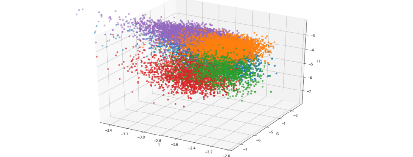
For a better understanding look at the output of the following code snipplet where only three letters already lead to a noticable form of clustering:

projection='3d')
legend = []
X, Y, Z = 'e', 'g', 'h'

def iterlog(ln):
    retvals = []
    for n in ln:
        try:
            retvals.append(np.log(n))
        except:
            retvals.append(None)
    return retvals

for X in ['t']:
    ax = plt.axes(projection='3d')
    ax.xy_viewLim.intervalx = [-3.5, -2]
    legend = []
    for lang in [l for l in df.groupby('lang') if l[0] in {'German', 'English', 'Finnish', 'French', 'Danish'}]:
        sample = lang[1].sample(4000)

        legend.append(lang[0])
        ax.scatter3D(iterlog(sample[X]), iterlog(sample[Y]), iterlog(sample[Z]))

    ax.set_title('log(10) of the Relativ Frequencies of "' + X.upper() + "', '" + Y.upper() + '" and "' + Z.upper() + '"\n\n')
    ax.set_xlabel(X.upper())
    ax.set_ylabel(Y.upper())
    ax.set_zlabel(Z.upper())
    plt.legend(legend)
    plt.show()


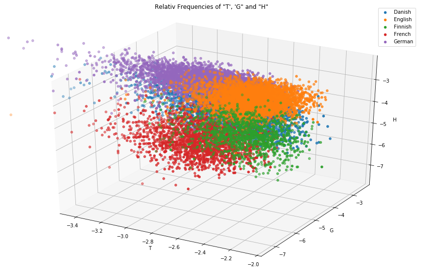
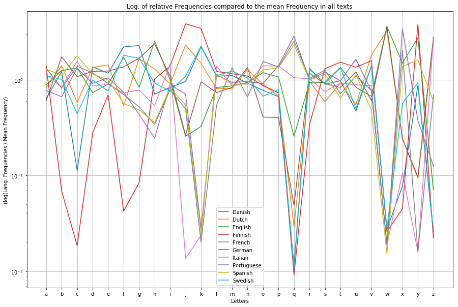
Even though every single letter frequency by itself is not a very reliable indicator, the set of frequencies of all present letters in a text is a quite good evidence because it will more or less represent the letter frequency fingerprint of the given language. Since it is quite hard to imagine or visualize the above plot in more than three dimensions, I used a little trick which shows that every language has its own typical fingerprint of letter frequencies:

legend = []
fig = plt.figure(figsize=(15, 10))
plt.axes(yscale='log')
    
langs = defaultdict(list)

for lang in [l for l in df.groupby('lang') if l[0] in set(df['lang'])]:
    for feature in 'abcdefghijklmnopqrstuvwxyz':
        langs[lang[0]].append(lang[1][feature].mean())

mean_frequencies = {feature:df[feature].mean() for feature in 'abcdefghijklmnopqrstuvwxyz'}
for i in langs.items():
    legend.append(i[0])
    j = np.array(i[1]) / np.array([mean_frequencies[c] for c in 'abcdefghijklmnopqrstuvwxyz'])
    plt.plot([c for c in 'abcdefghijklmnopqrstuvwxyz'], j)
plt.title('Log. of relative Frequencies compared to the mean Frequency in all texts')
plt.xlabel('Letters')
plt.ylabel('(log(Lang. Frequencies / Mean Frequency)')
plt.legend(legend)
plt.grid()
plt.show()

What more?

Beside the fact, that letter frequencies alone, allow us to predict the language of every example text (at least in the 10 languages with latin alphabet we trained for) with almost complete certancy there is even more information hidden in the set of sample texts.

As you might know, most languages in europe belong to either the romanian or the indogermanic language family (which is actually because the romans conquered only half of europe). The border between them could be located in belgium, between france and germany and in swiss. West of this border the romanian languages, which originate from latin, are still spoken, like spanish, portouguese and french. In the middle and northern part of europe the indogermanic languages are very common like german, dutch, swedish ect. If we plot the analysed languages with a different colour sheme this border gets quite clear and allows us to take a look back in history that tells us where our languages originate from:

legend = []
fig = plt.figure(figsize=(15, 10))
plt.axes(yscale='linear')
    
langs = defaultdict(list)
for lang in [l for l in df.groupby('lang') if l[0] in {'German', 'English', 'French', 'Spanish', 'Portuguese', 'Dutch', 'Swedish', 'Danish', 'Italian'}]:
    for feature in 'abcdefghijklmnopqrstuvwxyz':
        langs[lang[0]].append(lang[1][feature].mean())

colordict = {l[0]:l[1] for l in zip([lang for lang in langs], ['brown', 'tomato', 'orangered',
                                                               'green', 'red', 'forestgreen', 'limegreen',
                                                               'darkgreen', 'darkred'])}
mean_frequencies = {feature:df[feature].mean() for feature in 'abcdefghijklmnopqrstuvwxyz'}
for i in langs.items():
    legend.append(i[0])
    j = np.array(i[1]) / np.array([mean_frequencies[c] for c in 'abcdefghijklmnopqrstuvwxyz'])
    plt.plot([c for c in 'abcdefghijklmnopqrstuvwxyz'], j, color=colordict[i[0]])
#     plt.plot([c for c in 'abcdefghijklmnopqrstuvwxyz'], i[1], color=colordict[i[0]])
plt.title('Log. of relative Frequencies compared to the mean Frequency in all texts')
plt.xlabel('Letters')
plt.ylabel('(log(Lang. Frequencies / Mean Frequency)')
plt.legend(legend)
plt.grid()
plt.show()

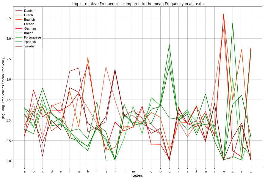
As you can see the more common letters, especially the vocals like a, e, i, o and u have almost the same frequency in all of this languages. Far more interesting are letters like q, k, c and w: While k is quite common in all of the indogermanic languages it is quite rare in romanic languages because the same sound is written with the letters q or c.
As a result it could be said, that even “boring” sets of data (just give it a try and read all the texts of the protocolls of the EU parliament…) could contain quite interesting patterns which – in this case – allows us to predict quite precisely which language a given text sample is written in, without the need of any translation program or to speak the languages. And as an interesting side effect, where certain things in history happend (or not happend): After two thousand years have passed, modern machine learning techniques could easily uncover this history because even though all these different languages developed, they still have a set of hidden but common patterns that since than stayed the same.

Sentiment Analysis using Python

One of the applications of text mining is sentiment analysis. Most of the data is getting generated in textual format and in the past few years, people are talking more about NLP. Improvement is a continuous process and many product based companies leverage these text mining techniques to examine the sentiments of the customers to find about what they can improve in the product. This information also helps them to understand the trend and demand of the end user which results in Customer satisfaction.

As text mining is a vast concept, the article is divided into two subchapters. The main focus of this article will be calculating two scores: sentiment polarity and subjectivity using python. The range of polarity is from -1 to 1(negative to positive) and will tell us if the text contains positive or negative feedback. Most companies prefer to stop their analysis here but in our second article, we will try to extend our analysis by creating some labels out of these scores. Finally, a multi-label multi-class classifier can be trained to predict future reviews.

Without any delay let’s deep dive into the code and mine some knowledge from textual data.

There are a few NLP libraries existing in Python such as Spacy, NLTK, gensim, TextBlob, etc. For this particular article, we will be using NLTK for pre-processing and TextBlob to calculate sentiment polarity and subjectivity.

import pandas as pd
import matplotlib.pyplot as plt
%matplotlib inline  
import nltk
from nltk import word_tokenize, sent_tokenize
from nltk.corpus import stopwords
from nltk.stem import LancasterStemmer, WordNetLemmatizer, PorterStemmer
from wordcloud import WordCloud, STOPWORDS
from textblob import TextBlob

The dataset is available here for download and we will be using pandas read_csv function to import the dataset. I would like to share an additional information here which I came to know about recently. Those who have already used python and pandas before they probably know that read_csv is by far one of the most used function. However, it can take a while to upload a big file. Some folks from  RISELab at UC Berkeley created Modin or Pandas on Ray which is a library that speeds up this process by changing a single line of code.

amz_reviews = pd.read_csv("1429_1.csv")

After importing the dataset it is recommended to understand it first and study the structure of the dataset. At this point we are interested to know how many columns are there and what are these columns so I am going to check the shape of the data frame and go through each column name to see if we need them or not.

amz_reviews.shape
(34660, 21)

amz_reviews.columns
Index(['id', 'name', 'asins', 'brand', 'categories', 'keys', 'manufacturer',
       'reviews.date', 'reviews.dateAdded', 'reviews.dateSeen',
       'reviews.didPurchase', 'reviews.doRecommend', 'reviews.id',
       'reviews.numHelpful', 'reviews.rating', 'reviews.sourceURLs',
       'reviews.text', 'reviews.title', 'reviews.userCity',
       'reviews.userProvince', 'reviews.username'],
      dtype='object')


There are so many columns which are not useful for our sentiment analysis and it’s better to remove these columns. There are many ways to do that: either just select the columns which you want to keep or select the columns you want to remove and then use the drop function to remove it from the data frame. I prefer the second option as it allows me to look at each column one more time so I don’t miss any important variable for the analysis.

columns = ['id','name','keys','manufacturer','reviews.dateAdded', 'reviews.date','reviews.didPurchase',
          'reviews.userCity', 'reviews.userProvince', 'reviews.dateSeen', 'reviews.doRecommend','asins',
          'reviews.id', 'reviews.numHelpful', 'reviews.sourceURLs', 'reviews.title']

df = pd.DataFrame(amz_reviews.drop(columns,axis=1,inplace=False))

Now let’s dive deep into the data and try to mine some knowledge from the remaining columns. The first step we would want to follow here is just to look at the distribution of the variables and try to make some notes. First, let’s look at the distribution of the ratings.

df['reviews.rating'].value_counts().plot(kind='bar')

Graphs are powerful and at this point, just by looking at the above bar graph we can conclude that most people are somehow satisfied with the products offered at Amazon. The reason I am saying ‘at’ Amazon is because it is just a platform where anyone can sell their products and the user are giving ratings to the product and not to Amazon. However, if the user is satisfied with the products it also means that Amazon has a lower return rate and lower fraud case (from seller side). The job of a Data Scientist relies not only on how good a model is but also on how useful it is for the business and that’s why these business insights are really important.

Data pre-processing for textual variables

Lowercasing

Before we move forward to calculate the sentiment scores for each review it is important to pre-process the textual data. Lowercasing helps in the process of normalization which is an important step to keep the words in a uniform manner (Welbers, et al., 2017, pp. 245-265).

## Change the reviews type to string
df['reviews.text'] = df['reviews.text'].astype(str)

## Before lowercasing 
df['reviews.text'][2]
'Inexpensive tablet for him to use and learn on, step up from the NABI. He was thrilled with it, learn how to Skype on it 
already...'

## Lowercase all reviews
df['reviews.text'] = df['reviews.text'].apply(lambda x: " ".join(x.lower() for x in x.split()))
df['reviews.text'][2] ## to see the difference
'inexpensive tablet for him to use and learn on, step up from the nabi. he was thrilled with it, learn how to skype on it 
already...'

Special characters

Special characters are non-alphabetic and non-numeric values such as {!,@#$%^ *()~;:/<>|+_-[]?}. Dealing with numbers is straightforward but special characters can be sometimes tricky. During tokenization, special characters create their own tokens and again not helpful for any algorithm, likewise, numbers.

## remove punctuation
df['reviews.text'] = df['reviews.text'].str.replace('[^ws]','')
df['reviews.text'][2]
'inexpensive tablet for him to use and learn on step up from the nabi he was thrilled with it learn how to skype on it already'

Stopwords

Stop-words being most commonly used in the English language; however, these words have no predictive power in reality. Words such as I, me, myself, he, she, they, our, mine, you, yours etc.

stop = stopwords.words('english')
df['reviews.text'] = df['reviews.text'].apply(lambda x: " ".join(x for x in x.split() if x not in stop))
df['reviews.text'][2]
'inexpensive tablet use learn step nabi thrilled learn skype already'

Stemming

Stemming algorithm is very useful in the field of text mining and helps to gain relevant information as it reduces all words with the same roots to a common form by removing suffixes such as -action, ing, -es and -ses. However, there can be problematic where there are spelling errors.

st = PorterStemmer()
df['reviews.text'] = df['reviews.text'].apply(lambda x: " ".join([st.stem(word) for word in x.split()]))
df['reviews.text'][2]
'inexpens tablet use learn step nabi thrill learn skype alreadi'

This step is extremely useful for pre-processing textual data but it also depends on your goal. Here our goal is to calculate sentiment scores and if you look closely to the above code words like ‘inexpensive’ and ‘thrilled’ became ‘inexpens’ and ‘thrill’ after applying this technique. This will help us in text classification to deal with the curse of dimensionality but to calculate the sentiment score this process is not useful.

Sentiment Score

It is now time to calculate sentiment scores of each review and check how these scores look like.

## Define a function which can be applied to calculate the score for the whole dataset

def senti(x):
    return TextBlob(x).sentiment  

df['senti_score'] = df['reviews.text'].apply(senti)

df.senti_score.head()

0                                   (0.3, 0.8)
1                                (0.65, 0.675)
2                                   (0.0, 0.0)
3    (0.29545454545454547, 0.6492424242424243)
4                    (0.5, 0.5827777777777777)
Name: senti_score, dtype: object

As it can be observed there are two scores: the first score is sentiment polarity which tells if the sentiment is positive or negative and the second score is subjectivity score to tell how subjective is the text. The whole code is available here.

In my next article, we will extend this analysis by creating labels based on these scores and finally we will train a classification model.

Sentiment Analysis using Python

One of the applications of text mining is sentiment analysis. Most of the data is getting generated in textual format and in the past few years, people are talking more about NLP. Improvement is a continuous process many product based companies leverage these text mining techniques to examine the sentiments of the customers to find about what they can improve in the product. This information also helps them to understand the trend and demand of the end user which results in Customer satisfaction.

As text mining is a vast concept, the article is divided into two subchapters. The main focus of this article will be calculating two scores: sentiment polarity and subjectivity using python. The range of polarity is from -1 to 1(negative to positive) and will tell us if the text contains positive or negative feedback. Most companies prefer to stop their analysis here but in our second article, we will try to extend our analysis by creating some labels out of these scores. Finally, a multi-label multi-class classifier can be trained to predict future reviews.

Without any delay let’s deep dive into the code and mine some knowledge from textual data.

There are a few NLP libraries existing in Python such as Spacy, NLTK, gensim, TextBlob, etc. For this particular article, we will be using NLTK for pre-processing and TextBlob to calculate sentiment polarity and subjectivity.

import pandas as pd
import matplotlib.pyplot as plt
%matplotlib inline  
import nltk
from nltk import word_tokenize, sent_tokenize
from nltk.corpus import stopwords
from nltk.stem import LancasterStemmer, WordNetLemmatizer, PorterStemmer
from wordcloud import WordCloud, STOPWORDS
from textblob import TextBlob

The dataset is available here for download and we will be using pandas read_csv function to import the dataset. I would like to share an additional information here which I came to know about recently. Those who have already used python and pandas before they probably know that read_csv is by far one of the most used function. However, it can take a while to upload a big file. Some folks from  RISELab at UC Berkeley created Modin or Pandas on Ray which is a library that speeds up this process by changing a single line of code.

amz_reviews = pd.read_csv("1429_1.csv")

After importing the dataset it is recommended to understand it first and study the structure of the dataset. At this point we are interested to know how many columns are there and what are these columns so I am going to check the shape of the data frame and go through each column name to see if we need them or not.

amz_reviews.shape
(34660, 21)

amz_reviews.columns
Index(['id', 'name', 'asins', 'brand', 'categories', 'keys', 'manufacturer',
       'reviews.date', 'reviews.dateAdded', 'reviews.dateSeen',
       'reviews.didPurchase', 'reviews.doRecommend', 'reviews.id',
       'reviews.numHelpful', 'reviews.rating', 'reviews.sourceURLs',
       'reviews.text', 'reviews.title', 'reviews.userCity',
       'reviews.userProvince', 'reviews.username'],
      dtype='object')


There are so many columns which are not useful for our sentiment analysis and it’s better to remove these columns. There are many ways to do that: either just select the columns which you want to keep or select the columns you want to remove and then use the drop function to remove it from the data frame. I prefer the second option as it allows me to look at each column one more time so I don’t miss any important variable for the analysis.

columns = ['id','name','keys','manufacturer','reviews.dateAdded', 'reviews.date','reviews.didPurchase',
          'reviews.userCity', 'reviews.userProvince', 'reviews.dateSeen', 'reviews.doRecommend','asins',
          'reviews.id', 'reviews.numHelpful', 'reviews.sourceURLs', 'reviews.title']

df = pd.DataFrame(amz_reviews.drop(columns,axis=1,inplace=False))

Now let’s dive deep into the data and try to mine some knowledge from the remaining columns. The first step we would want to follow here is just to look at the distribution of the variables and try to make some notes. First, let’s look at the distribution of the ratings.

df['reviews.rating'].value_counts().plot(kind='bar')

Graphs are powerful and at this point, just by looking at the above bar graph we can conclude that most people are somehow satisfied with the products offered at Amazon. The reason I am saying ‘at’ Amazon is because it is just a platform where anyone can sell their products and the user are giving ratings to the product and not to Amazon. However, if the user is satisfied with the products it also means that Amazon has a lower return rate and lower fraud case (from seller side). The job of a Data Scientist relies not only on how good a model is but also on how useful it is for the business and that’s why these business insights are really important.

Data pre-processing for textual variables

Lowercasing

Before we move forward to calculate the sentiment scores for each review it is important to pre-process the textual data. Lowercasing helps in the process of normalization which is an important step to keep the words in a uniform manner (Welbers, et al., 2017, pp. 245-265).

## Change the reviews type to string
df['reviews.text'] = df['reviews.text'].astype(str)

## Before lowercasing 
df['reviews.text'][2]
'Inexpensive tablet for him to use and learn on, step up from the NABI. He was thrilled with it, learn how to Skype on it 
already...'

## Lowercase all reviews
df['reviews.text'] = df['reviews.text'].apply(lambda x: " ".join(x.lower() for x in x.split()))
df['reviews.text'][2] ## to see the difference
'inexpensive tablet for him to use and learn on, step up from the nabi. he was thrilled with it, learn how to skype on it 
already...'

Special characters

Special characters are non-alphabetic and non-numeric values such as {!,@#$%^ *()~;:/<>|+_-[]?}. Dealing with numbers is straightforward but special characters can be sometimes tricky. During tokenization, special characters create their own tokens and again not helpful for any algorithm, likewise, numbers.

## remove punctuation
df['reviews.text'] = df['reviews.text'].str.replace('[^ws]','')
df['reviews.text'][2]
'inexpensive tablet for him to use and learn on step up from the nabi he was thrilled with it learn how to skype on it already'

Stopwords

Stop-words being most commonly used in the English language; however, these words have no predictive power in reality. Words such as I, me, myself, he, she, they, our, mine, you, yours etc.

stop = stopwords.words('english')
df['reviews.text'] = df['reviews.text'].apply(lambda x: " ".join(x for x in x.split() if x not in stop))
df['reviews.text'][2]
'inexpensive tablet use learn step nabi thrilled learn skype already'

Stemming

Stemming algorithm is very useful in the field of text mining and helps to gain relevant information as it reduces all words with the same roots to a common form by removing suffixes such as -action, ing, -es and -ses. However, there can be problematic where there are spelling errors.

st = PorterStemmer()
df['reviews.text'] = df['reviews.text'].apply(lambda x: " ".join([st.stem(word) for word in x.split()]))
df['reviews.text'][2]
'inexpens tablet use learn step nabi thrill learn skype alreadi'

This step is extremely useful for pre-processing textual data but it also depends on your goal. Here our goal is to calculate sentiment scores and if you look closely to the above code words like ‘inexpensive’ and ‘thrilled’ became ‘inexpens’ and ‘thrill’ after applying this technique. This will help us in text classification to deal with the curse of dimensionality but to calculate the sentiment score this process is not useful.

Sentiment Score

It is now time to calculate sentiment scores of each review and check how these scores look like.

## Define a function which can be applied to calculate the score for the whole dataset

def senti(x):
    return TextBlob(x).sentiment  

df['senti_score'] = df['reviews.text'].apply(senti)

df.senti_score.head()

0                                   (0.3, 0.8)
1                                (0.65, 0.675)
2                                   (0.0, 0.0)
3    (0.29545454545454547, 0.6492424242424243)
4                    (0.5, 0.5827777777777777)
Name: senti_score, dtype: object

As it can be observed there are two scores: the first score is sentiment polarity which tells if the sentiment is positive or negative and the second score is subjectivity score to tell how subjective is the text.

In my next article, we will extend this analysis by creating labels based on these scores and finally we will train a classification model.

Deep Learning and Human Intelligence – Part 2 of 2

Data dependency is one of the biggest problem of Deep Learning Architectures. This difficulty lies not so much in the algorithm of Deep Learning as in the invisible structure of the data itself.

This is part 2 of 2 of the Article Series: Deep Learning and Human Intelligence.

We saw that the process of discovering numbers was accompanied with many aspects of what are today basic ideas of Machine Learning. But let us go back, a little before that time, when humankind did not fully discovered the concept of numbers. How would a person, at such a time, perceive quantity and the count of things? Some structures are easily recognizable as patterns of objects, that is numbers, like one sun, 2 trees, 3 children, 4 clouds and so on. Sets of objects are much simpler to count if all the objects of the set are present. In such a case it is sufficient to keep a one-to-one relationship between two different set, without the need for numbers, to make a judgement of crucial importance. One could consider the case of two enemies that go to war and wish to know which has a larger army. It is enough to associate a small stone to every enemy soldier and do the same with his one soldier to be able to decide, depending if stones are left or not, if his army is larger or not, without ever needing to know the exact number soldier of any of the armies.

But also does things can be counted which are not directly visible, and do not allow a direct association with direct observable objects that can be seen, like stones. Would a person, at that time, be able to observe easily the 4-th day since today, 5 weeks from now, when even the concept of week is already composite? Counting in this case is only possible if numbers are already developed through direct observation, and we use something similar with stones in our mind, i.e. a cognitive association, a number. Only then, one can think of the concept of measuring at equidistant moments in time at all. This is the reason why such measurements where still cutting edge in the time of Galileo Galilei as we seen before. It is easily to assume that even in the time when humans started to count, such indirect concepts of numbers were not considered to be in relation with numbers. This implies that many concepts with which we are today accustomed to regard as a number, were considered as belonging to different groups, cluster which are not related. Such an hypothesis is not even that much farfetched. Evidence for such a time are still present in some languages, like Japanese.

When we think of numbers, we associate them with the Indo-Arabic numbers, but in Japanese numbers have no decimal structure and counting depends not only on the length of the set (which is usually considered as the number), but also on the objects that make up the set. In Japanese one can speak of meeting roku people, visiting muttsu cities and seeing ropa birds, but referring each time to the same number: six. Additional, many regular or irregular suffixes make the whole system quite complicated. The division of counting into so many clusters seems unnecessarily complicated today, but can easily be understood from a point of view where language and numbers still form and, the numbers, were not yet a uniform concept. What one can learn from this is that the lack of a unifying concept implies an overly complex dependence on data, which is the present case for Deep Learning and AI in general.

Although Deep Learning was a breakthrough in the development of Artificial Intelligence, the task such algorithms can perform were and remained very narrow. It may identify birds or cancer cells, but it will miss the song of the birds or the cry of the patient with cancer. When Watson, a Deep Learning Architecture played the famous Jeopardy game against two former Champions and won, it still made several simple mistakes, like going for the same wrong answer like the player before. If it could listen to the answer of the candidate, it could delete the top answer it had, and gibe the second which was the right one. With other words, Deep Learning Architecture are not multi-tasking and it is for this reason that some experts in AI are calling them intelligent idiots.

Imagine spending time learning to play a game for years and years, and then, when mastering it and wish to play a different game, to be unable to use any of the past experience (of gaming) for the new one and needing to learn everything from scratch. That could be quite depressing and would make life needlessly difficult. This is the reason why people involved in developing Deep Learning worked from early on in the development of multi-tasking Deep Learning Architectures. On the way a different method of using Deep Learning was discovered: transfer learning. Because the time it takes for a Deep Learning Architecture to learn is very long, transfer learning uses already learned Deep Learning Architectures but for slightly different task. It is similar to the use of past experiences in solving new problems, but, the advantage of transfer learning is, it allow the using of past experiences (what it already learned) which reduces dramatically the amount of new data needed in performing a new task. Still, transfer learning is far away from permitting Deep Learning Architectures to perform any kind of task learning only from one master data set.

The management of a unique master data set which includes all the needed data to enable human accuracy for any human activity, is not enough. One needs another ingredient, the so called cost function which translates, in this case, to the human brain. There are all our experiences and knowledge. How long does it takes to collect sufficient of both to handle a normal human life? How much to achieve our highest potential? If not a lifetime, at least decades. And this also applies to our job: as a IT-developer, a Data Scientist or a professor at the university. We will always have to learn new things, how to use them, and how to expand the limits of our perceptions. The vast amount of information that science has gathered over the last four centuries makes it impossible for any human being to become an expert in all of it. Thus, one has to specialized. After the university, anyone has to choose o subject which is appealing enough to study it for decades. Here is the first sign of what can be understood as data segmentation and dependency. Such improvements can come in various forms: an algorithm in the IT, a theorem in mathematics, a new way to look at particles in physics or a new method to scan for diseases in biology, and so on. But there is a price to pay for specialization: the inability to be an expert in another field or subfield. (Subfields induces limitation!)

Lets take the Deep Learning algorithm itself as an example. For IT and much of everyday life, this is a real breakthrough, but it lacks any scientific, that is mathematical, foundation. There are no theorems which proofs that it will find (converge, to use a mathematical term) the global optimum. This does not appear to be of any great consequences if it can be so efficient, except that, when adding new data and let the algorithm learn the same architecture again, there is no guaranty what so ever that it will be as good as the old model, or even better. On the contrary, it is as real as the efficiency of the first model, that chances are that the new model with the new data will perform worse than the old model, and one has to invest again time in finding a better model, or even a different architecture. On the other hand, with a mathematical proof of convergence, it would be always possible to know in what condition such a convergence can be achieved. In other words, without deep knowledge in mathematics, any proof of a consistent Deep Learning Algorithm is impossible.

Such a situation is true for any other corssover between fields. A mathematical genius will make a lousy biologist, a great chemist will make a average economist, and a top economist will be a poor physicist. Knowledge is difficult to transfer and this is true also for everyday experiences. We learn from very small to play a game like football, but are unable to use the reflexes to play basketball, or tennis better than a normal beginner. We learn a new language after years and years of practice, but are unable to use the way we learned to learn faster other languages. We are trapped within the knowledge we developed from the data we used. It is for this reason why we cannot transfer the knowledge a mathematician has developed over decades to use it in biology or psychology, even if the knowledge is very advanced. Instead of thinking in knowledge, we thing in data. This is similar to the people which were unaware of numbers, and used sets (data) to work with them. Numbers could be very difficult to transmit from one person to another in former times.

Only think on all the great achievements that our society managed, like relativity, quantum mechanics, DNA, machines, etc. Such discoveries are the essences of human knowledge and took millennia to form and centuries to crystalize. Still, all this knowledge is captive in the data, in the special frame in which it was discovered and never had the chance to escape. Imagine the possibility to use thoughts/causalities like the one in relativity or quantum mechanics in biology, or history, or of the concept of DNA in mathematics or art. Imagine a music composition where the law of the notes allows a “tunnel effect” like in quantum mechanics, lower notes to warp the music scales like in relativity and/or to twist two music scale in a helix-like play. How many way to experience life awaits us. Or think of the knowledge hidden in mathematics which could help develop new medicine, but can not be transmitted.

Another example of the connection we experience between knowledge and the data through which we obtain it, are children. They are classical example when it come determine if one is up to explain to them something. Take as an explain something simple they can observe often, like lightning and thunder. Normal concepts like particles, charge, waves, propagation, medium of propagation, etc. become so complicated to expose by other means then the one through which they were discovered, that it becomes nearly impossible to explain to children how it works and that they do not need to fear it. Still, one can use analogy (i.e., transfer) to enable an explanation. Instead of particles, one can use balls, for charge one can use hardness, waves can be shown with strings by keeping one end fix and waving the other, propagation is the movement of the waves from one end of the string to the other end, medium of propagation is the difference between walking in air and water, etc. Although difficult, analogies can be found which enables us to explain even to children how complex phenomena works.

The same is true also for Deep Learning. The model, the knowledge it can extract from the data can be expressed only by such data alone. There is no transformation of the knowledge from one type of data to another. If such a transformation would exists, then Deep Learning would be able to learn any human task by only a set of data, a master data set. Without such a master data set and a corresponding cost function it will be nearly impossible to develop AI that mimics human behavior. With other words, without the realization how our mind works, and how to crystalize by this the data needed, AI will still need to look at all the activities separately. It also implies that AI are restricted to the human understanding of reality and themselves. Only with such a characteristic of a living being, thus also AI, can development of its on occur.

How To Remotely Send R and Python Execution to SQL Server from Jupyter Notebooks

Introduction

Did you know that you can execute R and Python code remotely in SQL Server from Jupyter Notebooks or any IDE? Machine Learning Services in SQL Server eliminates the need to move data around. Instead of transferring large and sensitive data over the network or losing accuracy on ML training with sample csv files, you can have your R/Python code execute within your database. You can work in Jupyter Notebooks, RStudio, PyCharm, VSCode, Visual Studio, wherever you want, and then send function execution to SQL Server bringing intelligence to where your data lives.

This tutorial will show you an example of how you can send your python code from Juptyter notebooks to execute within SQL Server. The same principles apply to R and any other IDE as well. If you prefer to learn through videos, this tutorial is also published on YouTube here:


Environment Setup Prerequisites

  1. Install ML Services on SQL Server

In order for R or Python to execute within SQL, you first need the Machine Learning Services feature installed and configured. See this how-to guide.

  1. Install RevoscalePy via Microsoft’s Python Client

In order to send Python execution to SQL from Jupyter Notebooks, you need to use Microsoft’s RevoscalePy package. To get RevoscalePy, download and install Microsoft’s ML Services Python Client. Documentation Page or Direct Download Link (for Windows).

After downloading, open powershell as an administrator and navigate to the download folder. Start the installation with this command (feel free to customize the install folder): .\Install-PyForMLS.ps1 -InstallFolder “C:\Program Files\MicrosoftPythonClient”

Be patient while the installation can take a little while. Once installed navigate to the new path you installed in. Let’s make an empty folder and open Jupyter Notebooks: mkdir JupyterNotebooks; cd JupyterNotebooks; ..\Scripts\jupyter-notebook

Create a new notebook with the Python 3 interpreter:


To test if everything is setup, import revoscalepy in the first cell and execute. If there are no error messages you are ready to move forward.

Database Setup (Required for this tutorial only)

For the rest of the tutorial you can clone this Jupyter Notebook from Github if you don’t want to copy paste all of the code. This database setup is a one time step to ensure you have the same data as this tutorial. You don’t need to perform any of these setup steps to use your own data.

  1. Create a database

Modify the connection string for your server and use pyodbc to create a new database.

import pyodbc  
# creating a new db to load Iris sample in 
new_db_name = "MLRemoteExec" connection_string = "Driver=SQL Server;Server=localhost\MSSQLSERVER2017;Database={0};Trusted_Connection=Yes;" 

cnxn = pyodbc.connect(connection_string.format("master"), autocommit=True) 

cnxn.cursor().execute("IF EXISTS(SELECT * FROM sys.databases WHERE [name] = '{0}') DROP DATABASE {0}".format(new_db_name)) 

cnxn.cursor().execute("CREATE DATABASE " + new_db_name)

cnxn.close()

print("Database created") 
  1. Import Iris sample from SkLearn

Iris is a popular dataset for beginner data science tutorials. It is included by default in sklearn package.

from sklearn import datasetsimport pandas as pd
# SkLearn has the Iris sample dataset built in to the packageiris = datasets.load_iris()
df = pd.DataFrame(iris.data, columns=iris.feature_names)
  1. Use RecoscalePy APIs to create a table and load the Iris data

(You can also do this with pyodbc, sqlalchemy or other packages)

from revoscalepy import RxSqlServerData, rx_data_step
# Example of using RX APIs to load data into SQL table. You can also do this with pyodbc
table_ref = RxSqlServerData(connection_string=connection_string.format(new_db_name), table="Iris")rx_data_step(input_data = df, output_file = table_ref, overwrite = True)print("New Table Created: Iris")
print("Sklearn Iris sample loaded into Iris table")

Define a Function to Send to SQL Server

Write any python code you want to execute in SQL. In this example we are creating a scatter matrix on the iris dataset and only returning the bytestream of the .png back to Jupyter Notebooks to render on our client.

def send_this_func_to_sql():
    from revoscalepy import RxSqlServerData, rx_import
    from pandas.tools.plotting import scatter_matrix
    import matplotlib.pyplot as plt
    import io    
# remember the scope of the variables in this func are within our SQL Server Python Runtime
    connection_string = "Driver=SQL Server;Server=localhost\MSSQLSERVER2017; Database=MLRemoteExec;Trusted_Connection=Yes;"

# specify a query and load into pandas dataframe df
    sql_query = RxSqlServerData(connection_string=connection_string, sql_query = "select * from Iris")

    df = rx_import(sql_query)
    scatter_matrix(df)

# return bytestream of image created by scatter_matrix
    buf = io.BytesIO()
    plt.savefig(buf, format="png")
    buf.seek(0)
    return buf.getvalue()

Send execution to SQL

Now that we are finally set up, check out how easy sending remote execution really is! First, import revoscalepy. Create a sql_compute_context, and then send the execution of any function seamlessly to SQL Server with RxExec. No raw data had to be transferred from SQL to the Jupyter Notebook. All computation happened within the database and only the image file was returned to be displayed.

from IPython import display
import matplotlib.pyplot as plt 
from revoscalepy import RxInSqlServer, rx_exec# create a remote compute context with connection to SQL Server

sql_compute_context = RxInSqlServer(connection_string=connection_string.format(new_db_name))

# use rx_exec to send the function execution to SQL Server

image = rx_exec(send_this_func_to_sql, compute_context=sql_compute_context)[0]

# only an image was returned to my jupyter client. All data remained secure and was manipulated in my db.

display.Image(data=image)

While this example is trivial with the Iris dataset, imagine the additional scale, performance, and security capabilities that you now unlocked. You can use any of the latest open source R/Python packages to build Deep Learning and AI applications on large amounts of data in SQL Server. We also offer leading edge, high-performance algorithms in Microsoft’s RevoScaleR and RevoScalePy APIs. Using these with the latest innovations in the open source world allows you to bring unparalleled selection, performance, and scale to your applications.

Learn More

Check out SQL Machine Learning Services Documentation to learn how you can easily deploy your R/Python code with SQL stored procedures making them accessible in your ETL processes or to any application. Train and store machine learning models in your database bringing intelligence to where your data lives.

Other YouTube Tutorials:

Interview – The Importance of Machine Learning for the Data Driven Business

To become more data-driven, organizations must mature their analytics and automate more of their decision making processes for innovation and differentiation. Data science seems like the right approach, yet is a new and fast moving field that seems to have as many dead ends as it has high ways to value. Cloudera Fast Forward Labs, led by Hilary Mason, shows companies the way.

Alice Albrecht is a research engineer at Cloudera Fast Forward Labs.  She spends her days researching the latest and greatest in machine learning and artificial intelligence and bringing that knowledge to working prototypes and delivering concrete advice for clients.  Prior to joining Fast Forward Labs, Alice worked in both finance and technology companies as a practicing data scientist, data science leader, and – most recently – a data product manager.  In addition to teaching machines to do cool things, Alice is passionate about mentoring and helping others grow in their careers.  Alice holds a PhD from Yale in cognitive neuroscience where she studied how humans summarize sensory information from the world around them and the neural substrates that underlie those summaries.

Read this article in German:
“Interview – Die Bedeutung von Machine Learning für das Data Driven Business“

Data Science Blog: Ms. Albrecht, you are a well-known keynote speaker for data science and artificial intelligence. While data science has arrived business already, deep learning seems to be the new trend. Is artificial intelligence for business already normal business or is it an overrated hype?

I’d say it isn’t either of those two options.  Data science is now widely adopted but companies still struggle to integrate this new discipline into their existing businesses.  As for deep learning, it really depends on the company that’s looking into using this technique.  I wouldn’t say that deep learning is by any means part of business as usual- nor should it be.  It’s a tool like any other and building a capacity for using a tool without clearly defined business needs is a recipe for disaster.

Data Science Blog: Just to make sure what we are talking about: What are the differences and overlaps between data analytics, data science, machine learning, deep learning and artificial intelligence?

Here at Cloudera Fast Forward Labs, we like to think of data analytics as collecting data and counting things (mostly for quick charts and reports).  Data science solves business problems by counting cleverly and predicting things with the data that’s collected.  Machine learning is about solving problems with new kinds of feedback loops that improve with more data.  Deep learning is a particular type of machine learning and is not itself a separate concept or type of tool.  Artificial intelligence taps into something more complicated than what we’re seeing today – it’s much broader than training machines to repetitively do very specialized tasks or solve very narrow problems.

Data Science Blog: And how can we add the context to big data?

From a theoretical perspective, data science has been around for decades. The building blocks for modern day machine learning, deep learning and artificial intelligence are based on mathematical theorems  that go back to the 1940’s and 1950’s. The challenge was that at the time, compute power and data storage capacity were simply too expensive for the approaches to be implemented. Today that’s all changed.. Not only has the cost of data storage dropped considerably, open source technology like Apache Hadoop has made it possible to store any volume of data at costs approaching zero. Compute power, even highly specialised chip architectures, are now also available on demand and only for the time organisations need them through public and private cloud solutions. The decreased cost of both data storage and compute power, together with a growing list of tools and resources readily available via the open source community allows companies of any size to benefit from data (no matter that size of that data).

Data Science Blog: What are the challenges for organizations in getting started with data science?

I see two big challenges when getting started with data science.  One is ensuring that you have organizational alignment around exactly what type of work data scientists will deliver (and timing for those projects).  The second hurdle is around ensuring that you have the right data in place before you start hiring data scientists. This can be tricky if you don’t have in-house expertise in this area, so sometimes it’s better to hire a data engineer or a data strategist (or director of data science) before you ever get started building out a data science team.

Data Science Blog: There are many discussions about how to build a data-driven business. Is it just about using data science to get a better understanding of customer behavior?

No, being data driven doesn’t just mean better understanding your customers (though that is one way that data science can help in an organization).  Aside from building an organization that relies on data and analytics to help them make decisions (about customer behavior or otherwise), being a data-driven business means that data is powering your core products.

Data Science Blog: The number of technologies, tools and frameworks is increasing. For organizations this also means increasing complexity. Do companies need to stay always up-to-date or could it be an advice to wait and imitate pioneers later?

While it’s not critical (or advisable) for organizations to adopt every new advancement that comes along, it is critical for them to stay abreast of emerging frameworks.  If a business waits to see what others are doing, and therefore don’t invest in understanding how new advancements can affect their particular business, they’ve likely already missed the boat.

Data Science Blog: Global players have big budgets just for doing research and setting up data labs. Middle-sized companies need to see the break even point soon. How can we accelerate the value generation of data science?

Having a team that is highly focused on a specific set of projects that are well-scoped and aligned to the business makes all the difference.  Data science and machine learning don’t have to sacrifice doing research and being innovative in order to produce value.  The biggest difference is that smaller teams will have to be more aware of how their choice of project fits into emerging frameworks and their particular acute and near term business needs.

Data Science Blog: How does Cloudera Fast Forward Labs help other organizations to accelerate their start with machine learning?

We advise organizations, based on their particular needs, on what the latest advancements are in machine learning and data science, how to build and structure their data teams to develop the capabilities they need to meet their goals, and how to quickly implement custom forward-looking solutions using their own data and in-house expertise.

Data Science Blog: Finally, a question for our younger readers who are looking for a career as a data expert: What makes a good data scientist? Do you like to work with introverted coding nerds or the data loving business experts?

A good data scientists should be deeply curious and have a love for the ways in which data can lead to new discoveries and power the next generation of products.  We expect the people who thrive in this field to come from a variety of backgrounds and experiences.

Deep Learning and Human Intelligence – Part 1 of 2

Many people are under the impression that the new wave of data science, machine learning and/or digitalization is new, that it did not exist before. But its history is as long as the history of humanity and/or science itself.  The scientific discovery could hardly take place without the necessary data. Even the process of discovering the numbers included elements of machine learning: pattern recognition, comparison between different groups (ranking), clustering, etc. So what differentiates mathematical formulas from machine learning and how does it relate to artificial intelligence?

There is no difference between the two if seen from the perspective of formulas however, such a perspective limits the type of data to which they can be applied. Data stored via tables consist of structured data and are stored in so-called relational databases. The reason for such a data storage is the connection between different fields that assume a well-established structure in advance, such as a company’s sales or balance sheet. However, with the emergence of personal computers, many of the daily activities have been digitalized: music, pictures, movies, and so on. All this information is stored unrelated to other data and therefore called unstructured data.

IEEE International Conference on Computer Vision (ICCV), 2015, DOI: 10.1109/ICCV.2015.428

Copyright: IEEE International Conference on Computer Vision (ICCV), 2015, DOI: 10.1109/ICCV.2015.428

The essence of scientific discoveries was and will be structure. Not surprisingly, the mathematical formulas revolve around relations between variables – information, in general. For example, Galileo derived the law of falling balls from measuring the successive hight of a falling ball. The main difficulty was to obtain measurements at regular time intervals. What about if the data is not structured, which mathematical formula should be applied then? There is a distribution of people’s height, but no distribution for the pictures taken in all holidays for the last year, there is an amplitude for acoustic signals, but no function that detects the similarity between two songs. This is one of the reasons why machine learning focuses heavily on clustering and classification.

Roughly speaking, these simple examples are enough to categorize the difference between scientific discovery and machine learning. Science is about discovering relationships between different variables, Machine Learning tries to automatize processes. Every technical improvement is part of the automation, so why is everything different in this case? Because the current automation deals with human intelligence. The car automates the walking, the kitchen stove the fire, but Machine Learning parts of the human intelligence. There is a difference between the previous automation steps and those of human intelligence. All the previous ones are either outside the human body – such as Fire – or unconsciously executed (once learned) – walking, spinning, etc. The automation induced by Machine Learning affects a part of the human intelligence that we consciously perceive. Of course, today’s machine learning tools are unable to automate all human intelligence, but it is a fascinating step in that direction.

A breakthrough in Machine Learning tasks was achieved in 2012 when the first Deep Learning algorithm for detecting types of images, reached near-human accuracy. It could appreciate the likelihood that the image is a human face, a train, a ball or a fish without having “seen” the picture before. Such an algorithm can be used in various areas:  personally – facial recognition in pictures and/or social media – as tagging of images or videos, medicine – cancer detection, etc. For understanding such cutting-edge issues of classification, one cannot avoid understanding how Deep Learning works. To see the beauty of such algorithms and, at the same time, to be able to comprehend the difficulty of working with them, an example will be the best guide.

The building blocks of Deep Learning are neurons, operational units, which perform mathematical operations or logical operations like AND, OR, etc., and are modelled after the neurons in the brain. Already in the 1950’s two neuroscientist, Hubel and Wiesel, observed that not all neurons in the brain are responding in the same fashion to visual stimuli. Some responded only to horizontal lines, whereas others to vertical lines, with other words, the brain is constructed with specialized neurons. Groups of such neurons are called, in the Machine Learning community, layers. Like in the brain, neurons with different properties are clustered in different layers. This implies that layers have also specific properties and have to be arranged in a specific way, called architecture. It is this architecture which differentiates Deep Learning from Artificial Neuronal Networks (ANN are similar to a layer).

Unfortunately, scientists still haven’t figured out how the brain works, thus to discover how to train Deep Learning from data was not an easy task, and is also the reason why another example is used to explain the training of Deep Learning: the eye. One has always to remember: once it is known how Deep Learning works, it is simple to find example which illustrates the working mechanism.  For such an analogy, it is sufficient for someone without any knowledge about Deep Learning, to keep in mind only the elements that compose such architectures: input data, different layers of neurons, output layers, ReLu’s.

Input data are any type of information, in our example it is light. Of course, that Deep Learning is not limited only to images or videos, but also to sound and/or time series, which would imply that the example would be the ear and sound waves, or the brain and numbers.

Layers can be seen as cells in the eye. It is well known that the eye is formed of different layers connected to each other with each of them having different properties, functionalities. The same is true also for the layers of a Deep Learning architecture: one can see the neurons as cells of the layer as the tissue. While, mathematically, the neurons are nothing more than simple operations, usually linear weight functions, they can be seen as the properties of individual cells. Each layer has one weight matrix, which gives the neuron (and layer) specific properties depending on the data and the task at hand.

It is here that the architecture becomes very important. What Deep Learning offers is a default setting of the layers with unknown weights. One can see this as trying to build an eye knowing that there are different types of cells and different ways how tissues of such cells can be arranged, but not which cell exactly is needed (with what properties) and which arrangement of layers works best. Such an approach has the advantage that one is capable of building any type of organ desired, but the disadvantage is also very obvious: it is time consuming to find the appropriate cell properties and layers arrangements.

Still, the strategy of Deep Learning is a significant departure from the Machine Learning approaches. The performance of Machine Learning methods is as good as the features engineering performed by Data Scientists, and thus depending on the creativity of the Data Scientist. In the case of Deep Learning the engineers of the features is performed automatically as part of the model building. This is a huge improvement, as the only difficult task is to have enough data and computer power to find the right weights matrices. Such an endeavor was performed also by nature for the eye — and is also the reason why one can choose it as an example for Deep Learning — evolution. It is not surprising that Deep Learning is one of the best direction scientists have of Artificial Intelligence today.

The evolution of the eye can be seen, from the perspective of Data Scientists, as the continuous training of a Deep Learning architecture which enables to recognize and track one or more objects. The performance of the evolutional process can be summed up as the fine tuning of the cells which are getting more and more susceptible to light and the adaptation of layers to enable a better vision. Different animals in different environments and different targets — as the hawk and the fly — developed different eyes than humans, but they all work according to the same principle. The tasks that Deep Learning is performing today are similar, for example it can be used to drive cars but there is still a difference:  there is no connection to other organs. Deep Learning is not the approximation of an Artificial Organism, like an android, but a simplified Artificial Organ that can work on its own.

Returning to the working mechanism of the Deep Learning architecture, we can already follow the analogy of what happens if a ray of light is hitting the eye. Once the eye is fully adapted to the task, one can followed how the information enters the Deep Learning architecture (Artificial Eye) by penetrating the input layer. already here arises the question, what kind of eye is the best? One where a small source of light can reach as many neurons as possible, or the one where the light sources reaches only few neurons? In order to take such a decision, a last piece of the puzzle is required: ReLu. One can see them as synapses between neurons (cells) and/or similarly for tissue. By using continuous functions, such as the shape of the latter ‘S’ (called sigmoid), the information from one neuron will be distributed over a large number of other neurons. If one uses the maximum function, then only few neurons are updated with processed information from earlier layers.

Such sparse structures between neurons, was a major improvement in the development of the technique of training Deep Learning architectures. Again, it has a strong evolutionary analogy: energy efficiency. By needing less neurons, the tissues and architecture are both kept to a minimal size which enables flexibility in development and less energy. As the information is process by the different layers, the Artificial Eye is gathering more and more complex (non-linear) structures — the adapted features –, which help to decide, from past experience, what kind of object is detected.

This was part 1 of 2 of the article series. Continue with Part 2.

Bringing intelligence to where data lives: Python & R embedded in T-SQL

Introduction

Did you know that you can write R and Python code within your T-SQL statements? Machine Learning Services in SQL Server eliminates the need for data movement. Instead of transferring large and sensitive data over the network or losing accuracy with sample csv files, you can have your R/Python code execute within your database. Easily deploy your R/Python code with SQL stored procedures making them accessible in your ETL processes or to any application. Train and store machine learning models in your database bringing intelligence to where your data lives.

You can install and run any of the latest open source R/Python packages to build Deep Learning and AI applications on large amounts of data in SQL Server. We also offer leading edge, high-performance algorithms in Microsoft’s RevoScaleR and RevoScalePy APIs. Using these with the latest innovations in the open source world allows you to bring unparalleled selection, performance, and scale to your applications.

If you are excited to try out SQL Server Machine Learning Services, check out the hands on tutorial below. If you do not have Machine Learning Services installed in SQL Server,you will first want to follow the getting started tutorial I published here: 

How-To Tutorial

In this tutorial, I will cover the basics of how to Execute R and Python in T-SQL statements. If you prefer learning through videos, I also published the tutorial on YouTube.

Basics

Open up SQL Server Management Studio and make a connection to your server. Open a new query and paste this basic example: (While I use Python in these samples, you can do everything with R as well)

EXEC sp_execute_external_script @language = N'Python',
@script = N'print(3+4)'

Sp_execute_external_script is a special system stored procedure that enables R and Python execution in SQL Server. There is a “language” parameter that allows us to choose between Python and R. There is a “script” parameter where we can paste R or Python code. If you do not see an output print 7, go back and review the setup steps in this article.

Parameter Introduction

Now that we discussed a basic example, let’s start adding more pieces:

EXEC sp_execute_external_script  @language =N'Python', 
@script = N' 
OutputDataSet = InputDataSet;
',
@input_data_1 =N'SELECT 1 AS Col1';

Machine Learning Services provides more natural communications between SQL and R/Python with an input data parameter that accepts any SQL query. The input parameter name is called “input_data_1”.
You can see in the python code that there are default variables defined to pass data between Python and SQL. The default variable names are “OutputDataSet” and “InputDataSet” You can change these default names like this example:

EXEC sp_execute_external_script  @language =N'Python', 
@script = N' 
MyOutput = MyInput;
',
@input_data_1_name = N'MyInput',
@input_data_1 =N'SELECT 1 AS foo',
@output_data_1_name =N'MyOutput';

As you executed these examples, you might have noticed that they each return a result with “(No column name)”? You can specify a name for the columns that are returned by adding the WITH RESULT SETS clause to the end of the statement which is a comma separated list of columns and their datatypes.

EXEC sp_execute_external_script  @language =N'Python', 
@script=N' 
MyOutput = MyInput;
',
@input_data_1_name = N'MyInput',
@input_data_1 =N'
SELECT 1 AS foo,
2 AS bar
',
@output_data_1_name =N'MyOutput'
WITH RESULT SETS ((MyColName int, MyColName2 int));

Input/Output Data Types

Alright, let’s discuss a little more about the input/output data types used between SQL and Python. Your input SQL SELECT statement passes a “Dataframe” to python relying on the Python Pandas package. Your output from Python back to SQL also needs to be in a Pandas Dataframe object. If you need to convert scalar values into a dataframe here is an example:

EXEC sp_execute_external_script  @language =N'Python', 
@script=N' 
import pandas as pd
c = 1/2
d = 1*2
s = pd.Series([c,d])
df = pd.DataFrame(s)
OutputDataSet = df
'

Variables c and d are both scalar values, which you can add to a pandas Series if you like, and then convert them to a pandas dataframe. This one shows a little bit more complicated example, go read up on the python pandas package documentation for more details and examples:

EXEC sp_execute_external_script  @language =N'Python', 
@script=N' 
import pandas as pd
s = {"col1": [1, 2], "col2": [3, 4]}
df = pd.DataFrame(s)
OutputDataSet = df
'

You now know the basics to execute Python in T-SQL!

Did you know you can also write your R and Python code in your favorite IDE like RStudio and Jupyter Notebooks and then remotely send the execution of that code to SQL Server? Check out these documentation links to learn more: https://aka.ms/R-RemoteSQLExecution https://aka.ms/PythonRemoteSQLExecution

Check out the SQL Server Machine Learning Services documentation page for more documentation, samples, and solutions. Check out these E2E tutorials on github as well.

Would love to hear from you! Leave a comment below to ask a question, or start a discussion!

OLAP Technology in Business Intelligence

Data in Business Intelligence
Business processes traditionally comprise three stages of data management: collecting, analyzing, and reporting. First, data should be gathered from all the sources through ETL tools (Extract, Transform, Load). After this, there are often issues occurring connected with data consistency hence the data should be cleaned and structured using the function of metadata. Once the data are provided to the end-user in a readable and transparent way it is ready to be analyzed. There are multiple applications ensuring data analysis including Data Mining, OLAP, BI. In order to carry out in-depth and coherent analysis, the best approach is to initially determine KPI as these are the criteria to assess the progress in relation to the goals set.

OLAP definition
OLAP tool belongs to Business Intelligence concept intended for big data management and is short for Online Analytical Processing. OLAP conducts multidimensional data analysis and enables end-users to perform complicated calculations, trend analysis, ‘what-if’ scenarios and the like. Furthermore, owing to OLAP it’s possible to conduct planning and forecasting, budgeting and financial reporting, analysis, and data modeling which contributes to successful decision making in business.

OLAP Structure
An OLAP cube is composed of dimensions containing aggregated information referred to and measures which include numerical data. Dimensions are arranged in hierarchies which in their turn are indicators to determine the rate of granularity; the rate is called a level. The most common dimensions are location, product, and time. The lowest granularity level of a time dimension may be hours while the highest one can present years. This way when there is a query to be responded the measures contribute to filter out the data and select the right object inside the dimension. In the center of the cube there is a star or a snowflake schema which all the dimensions refer to.

OLAP main characteristics
Here are the main features characterizing the OLAP tool”:

– The data in OLAP is structured as a multidimensional cube.
– The cube structure allows users to see the information from various angles given location, products, demographics, time, etc.
– Rapid data access and analysis due to precalculated aggregations.
– Simple and intuitive interface.
– OLAP doesn’t require IT skills or SQL knowledge (as some other business intelligence software tools). Hence its operation eases the burden of IT department.
– The tool supports complex custom calculations
– The OLAP databases maintain historical data and are updated not constantly but regularly.
– The cube design and building process is the pivotal step on the way to successful data processing.

OLAP requirements
When the OLAP technology was invented there were twelve rules generated to follow so that it complies with the concept of online data processing:

Multidimensional
Not only the OLAP view has to be multidimensional but the data should as well be stored in this way of structure in order to provide the multidimensional analysis.

Transparent
The architecture has to be transparent to let the user see and understand the functionality and the client server of the application.

Accessible
The end user must have an opportunity to access the information in its consistent view without any issues related to the sources where the data come from or the way the data are maintained in OLAP.

Consistent Reporting
The data are regularly upgraded and its volume grows progressively although the user shouldn’t see problems changes in the process of scheduled reporting regarding that.

Client-Server
OLAP application has to manage client-server architecture as it manages vast volumes of data often requiring a core server for storage and maintenance.

Common Dimensionality
The main feature of the dimension structure in OLAP must be the same for all the dimensions to keep the data consistent, accurate, valid, complete, etc. Thus the dimensions have to possess common operation capabilities and be equal in structure.

Dynamic Sparse Matrix Handling
A usual OLAP application must manage to deal with sparse matrices and shouldn’t let the cube expand excessively as a usual OLAP cube is relatively sparse.

Multi-User
OLAP technology is originally supposed to provide an opportunity to access the data for multiple users simultaneously. The process of data management must at the same time be ensured with security and integrity.

Unrestricted Cross-dimensional Operations
A typical OLAP application is meant to handle all calculations and operations (such as slice-and-dice, drill up-down, drill through etc.) without the participation of the user. Commonly the tool delivers a language to exploit while requiring specified information.

Intuitive Data Manipulation
All OLAP operations which handle dimensions, measures, hierarchies, levels etc. have to be user-friendly and easily adopted without requiring additional technical skills. An average employee is considered to cope with the data navigation and management through clear displaying and handy operations.

Flexible Reporting
The main function – reporting must be flexible with a view to organizing all the rows, columns, and page setup containing a requisite number of dimensions and hierarchies from the data. As a result, the user has to gain a report comprising all the needed members and the relations between them.

Unlimited Dimensions and Aggregation Levels
When the technology was designed it was intended to be able to contain up to twenty dimensions in the cube. Each dimension had to provide as many aggregation levels inside a hierarchy as required. The idea was to manage great volumes of data keeping end-users absolutely aware of the performance of the organization.

Advantages of OLAP
Speed
Before OLAP was invented and introduced to the market there hadn’t been a tool to rapidly run the queries and it had taken long to retrieve the required information from the data. Thus the main advantage of the OLAP application is its speed gained due to precomputation of the data aggregations.

MDX designer and ad-hoc reports
MDX Designer is aimed at creating interactive ad-hoc reports. The reports provide a better understanding of the business processes and the organization’s performance in the market.

Visualization
OLAP provides its users with sophisticated data analytics allowing them to see data from different perspectives. There are numerous formats to visualize the requisite data: pie charts, graphs, heat maps, reports, pyramids, etc. Moreover, OLAP includes a number of operations to handle data: rotate, drill up and down, slice and dice, etc. Besides, there’s also an opportunity to apply a ‘what-if’ scenario due to a write-back option. All mentioned above can significantly contribute to decision-making process regarding the ongoing situation.

Flexibility
OLAP table displayed is flexible with column and row labels depending on the requirements of the user. Moreover, the reporting generated is available in multiple dimensions.

Applying Data Science Techniques in Python to Evaluate Ionospheric Perturbations from Earthquakes

Multi-GNSS (Galileo, GPS, and GLONASS) Vertical Total Electron Content Estimates: Applying Data Science techniques in Python to Evaluate Ionospheric Perturbations from Earthquakes

1 Introduction

Today, Global Navigation Satellite System (GNSS) observations are routinely used to study the physical processes that occur within the Earth’s upper atmosphere. Due to the experienced satellite signal propagation effects the total electron content (TEC) in the ionosphere can be estimated and the derived Global Ionosphere Maps (GIMs) provide an important contribution to monitoring space weather. While large TEC variations are mainly associated with solar activity, small ionospheric perturbations can also be induced by physical processes such as acoustic, gravity and Rayleigh waves, often generated by large earthquakes.

In this study Ionospheric perturbations caused by four earthquake events have been observed and are subsequently used as case studies in order to validate an in-house software developed using the Python programming language. The Python libraries primarily utlised are Pandas, Scikit-Learn, Matplotlib, SciPy, NumPy, Basemap, and ObsPy. A combination of Machine Learning and Data Analysis techniques have been applied. This in-house software can parse both receiver independent exchange format (RINEX) versions 2 and 3 raw data, with particular emphasis on multi-GNSS observables from GPS, GLONASS and Galileo. BDS (BeiDou) compatibility is to be added in the near future.

Several case studies focus on four recent earthquakes measuring above a moment magnitude (MW) of 7.0 and include: the 11 March 2011 MW 9.1 Tohoku, Japan, earthquake that also generated a tsunami; the 17 November 2013 MW 7.8 South Scotia Ridge Transform (SSRT), Scotia Sea earthquake; the 19 August 2016 MW 7.4 North Scotia Ridge Transform (NSRT) earthquake; and the 13 November 2016 MW 7.8 Kaikoura, New Zealand, earthquake.

Ionospheric disturbances generated by all four earthquakes have been observed by looking at the estimated vertical TEC (VTEC) and residual VTEC values. The results generated from these case studies are similar to those of published studies and validate the integrity of the in-house software.

2 Data Cleaning and Data Processing Methodology

Determining the absolute VTEC values are useful in order to understand the background ionospheric conditions when looking at the TEC perturbations, however small-scale variations in electron density are of primary interest. Quality checking processed GNSS data, applying carrier phase leveling to the measurements, and comparing the TEC perturbations with a polynomial fit creating residual plots are discussed in this section.

Time delay and phase advance observables can be measured from dual-frequency GNSS receivers to produce TEC data. Using data retrieved from the Center of Orbit Determination in Europe (CODE) site (ftp://ftp.unibe.ch/aiub/CODE), the differential code biases are subtracted from the ionospheric observables.

2.1 Determining VTEC: Thin Shell Mapping Function

The ionospheric shell height, H, used in ionosphere modeling has been open to debate for many years and typically ranges from 300 – 400 km, which corresponds to the maximum electron density within the ionosphere. The mapping function compensates for the increased path length traversed by the signal within the ionosphere. Figure 1 demonstrates the impact of varying the IPP height on the TEC values.

Figure 1 Impact on TEC values from varying IPP heights. The height of the thin shell, H, is increased in 50km increments from 300 to 500 km.

2.2 Phase Smoothing

For dual-frequency GNSS users TEC values can be retrieved with the use of dual-frequency measurements by applying calculations. Calculation of TEC for pseudorange measurements in practice produces a noisy outcome and so the relative phase delay between two carrier frequencies – which produces a more precise representation of TEC fluctuations – is preferred. To circumvent the effect of pseudorange noise on TEC data, GNSS pseudorange measurements can be smoothed by carrier phase measurements, with the use of the carrier phase smoothing technique, which is often referred to as carrier phase leveling.

Figure 2 Phase smoothed code differential delay

2.3 Residual Determination

For the purpose of this study the monitoring of small-scale variations in ionospheric electron density from the ionospheric observables are of particular interest. Longer period variations can be associated with diurnal alterations, and changes in the receiver- satellite elevation angles. In order to remove these longer period variations in the TEC time series as well as to monitor more closely the small-scale variations in ionospheric electron density, a higher-order polynomial is fitted to the TEC time series. This higher-order polynomial fit is then subtracted from the observed TEC values resulting in the residuals. The variation of TEC due to the TID perturbation are thus represented by the residuals. For this report the polynomial order applied was typically greater than 4, and was chosen to emulate the nature of the arc for that particular time series. The order number selected is dependent on the nature of arcs displayed upon calculating the VTEC values after an initial inspection of the VTEC plots.

3 Results

3.1 Tohoku Earthquake

For this particular report, the sampled data focused on what was retrieved from the IGS station, MIZU, located at Mizusawa, Japan. The MIZU site is 39N 08′ 06.61″ and 141E 07′ 58.18″. The location of the data collection site, MIZU, and the earthquake epicenter can be seen in Figure 3.

Figure 3 MIZU IGS station and Tohoku earthquake epicenter [generated using the Python library, Basemap]

Figure 4 displays the ionospheric delay in terms of vertical TEC (VTEC), in units of TECU (1 TECU = 1016 el m-2). The plot is split into two smaller subplots, the upper section displaying the ionospheric delay (VTEC) in units of TECU, the lower displaying the residuals. The vertical grey-dashed lined corresponds to the epoch of the earthquake at 05:46:23 UT (2:46:23 PM local time) on March 11 2011. In the upper section of the plot, the blue line corresponds to the absolute VTEC value calculated from the observations, in this case L1 and L2 on GPS, whereby the carrier phase leveling technique was applied to the data set. The VTEC values are mapped from the STEC values which are calculated from the LOS between MIZU and the GPS satellite PRN18 (on Figure 4 denoted G18). For this particular data set as seen in Figure 4, a polynomial fit of  five degrees was applied, which corresponds to the red-dashed line. As an alternative to polynomial fitting, band-pass filtering can be employed when TEC perturbations are desired. However for the scope of this report polynomial fitting to the time series of TEC data was the only method used. In the lower section of Figure 4 the residuals are plotted. The residuals are simply the phase smoothed delay values (the blue line) minus the polynomial fit line (the red-dashed line). All ionosphere delay plots follow the same layout pattern and all time data is represented in UT (UT = GPS – 15 leap seconds, whereby 15 leap seconds correspond to the amount of leap seconds at the time of the seismic event). The time series shown for the ionosphere delay plots are given in terms of decimal of the hour, so that the format follows hh.hh.

Figure 4 VTEC and residual plot for G18 at MIZU on March 11 2011

3.2 South Georgia Earthquake

In the South Georgia Island region located in the North Scotia Ridge Transform (NSRT) plate boundary between the South American and Scotia plates on 19 August 2016, a magnitude of 7.4 MW earthquake struck at 7:32:22 UT. This subsection analyses the data retrieved from KEPA and KRSA. As well as computing the GPS and GLONASS TEC values, four Galileo satellites (E08, E14, E26, E28) are also analysed. Figure 5 demonstrates the TEC perturbations as computed for the Galileo L1 and L5 carrier frequencies.

Figure 5 VTEC and residual plots at KRSA on 19 August 2016. The plots are from the perspective of the GNSS receiver at KRSA, for four Galileo satellites (a) E08; (b) E14; (c) E24; (d) E26. The y-axes and x-axes in all plots do not conform with one another but are adjusted to fit the data. The y-axes for the residual section of each plot is consistent with one another.

Figure 6 Geometry of the Galileo (E08, E14, E24 and E26) satellites’ projected ground track whereby the IPP is set to 300km altitude. The orange lines correspond to tectonic plate boundaries.

4 Conclusion

The proximity of the MIZU site and magnitude of the Tohoku event has provided a remarkable – albeit a poignant – opportunity to analyse the ocean-ionospheric coupling aftermath of a deep submarine seismic event. The Tohoku event has also enabled the observation of the origin and nature of the TIDs generated by both a major earthquake and tsunami in close proximity to the epicenter. Further, the Python software developed is more than capable of providing this functionality, by drawing on its mathematical packages, such as NumPy, Pandas, SciPy, and Matplotlib, as well as employing the cartographic toolkit provided from the Basemap package, and finally by utilizing the focal mechanism generation library, Obspy.

Pre-seismic cursors have been investigated in the past and strongly advocated in particular by Kosuke Heki. The topic of pre-seismic ionospheric disturbances remains somewhat controversial. A potential future study area could be the utilization of the Python program – along with algorithmic amendments – to verify the existence of this phenomenon. Such work would heavily involve the use of Scikit-Learn in order to ascertain the existence of any pre-cursors.

Finally, the code developed is still retained privately and as of yet not launched to any particular platform, such as GitHub. More detailed information on this report can be obtained here:

Download as PDF