Sentiment Analysis using Python

One of the applications of text mining is sentiment analysis. Most of the data is getting generated in textual format and in the past few years, people are talking more about NLP. Improvement is a continuous process and many product based companies leverage these text mining techniques to examine the sentiments of the customers to find about what they can improve in the product. This information also helps them to understand the trend and demand of the end user which results in Customer satisfaction.

As text mining is a vast concept, the article is divided into two subchapters. The main focus of this article will be calculating two scores: sentiment polarity and subjectivity using python. The range of polarity is from -1 to 1(negative to positive) and will tell us if the text contains positive or negative feedback. Most companies prefer to stop their analysis here but in our second article, we will try to extend our analysis by creating some labels out of these scores. Finally, a multi-label multi-class classifier can be trained to predict future reviews.

Without any delay let’s deep dive into the code and mine some knowledge from textual data.

There are a few NLP libraries existing in Python such as Spacy, NLTK, gensim, TextBlob, etc. For this particular article, we will be using NLTK for pre-processing and TextBlob to calculate sentiment polarity and subjectivity.

import pandas as pd
import matplotlib.pyplot as plt
%matplotlib inline  
import nltk
from nltk import word_tokenize, sent_tokenize
from nltk.corpus import stopwords
from nltk.stem import LancasterStemmer, WordNetLemmatizer, PorterStemmer
from wordcloud import WordCloud, STOPWORDS
from textblob import TextBlob

The dataset is available here for download and we will be using pandas read_csv function to import the dataset. I would like to share an additional information here which I came to know about recently. Those who have already used python and pandas before they probably know that read_csv is by far one of the most used function. However, it can take a while to upload a big file. Some folks from  RISELab at UC Berkeley created Modin or Pandas on Ray which is a library that speeds up this process by changing a single line of code.

amz_reviews = pd.read_csv("1429_1.csv")

After importing the dataset it is recommended to understand it first and study the structure of the dataset. At this point we are interested to know how many columns are there and what are these columns so I am going to check the shape of the data frame and go through each column name to see if we need them or not.

amz_reviews.shape
(34660, 21)

amz_reviews.columns
Index(['id', 'name', 'asins', 'brand', 'categories', 'keys', 'manufacturer',
       'reviews.date', 'reviews.dateAdded', 'reviews.dateSeen',
       'reviews.didPurchase', 'reviews.doRecommend', 'reviews.id',
       'reviews.numHelpful', 'reviews.rating', 'reviews.sourceURLs',
       'reviews.text', 'reviews.title', 'reviews.userCity',
       'reviews.userProvince', 'reviews.username'],
      dtype='object')


There are so many columns which are not useful for our sentiment analysis and it’s better to remove these columns. There are many ways to do that: either just select the columns which you want to keep or select the columns you want to remove and then use the drop function to remove it from the data frame. I prefer the second option as it allows me to look at each column one more time so I don’t miss any important variable for the analysis.

columns = ['id','name','keys','manufacturer','reviews.dateAdded', 'reviews.date','reviews.didPurchase',
          'reviews.userCity', 'reviews.userProvince', 'reviews.dateSeen', 'reviews.doRecommend','asins',
          'reviews.id', 'reviews.numHelpful', 'reviews.sourceURLs', 'reviews.title']

df = pd.DataFrame(amz_reviews.drop(columns,axis=1,inplace=False))

Now let’s dive deep into the data and try to mine some knowledge from the remaining columns. The first step we would want to follow here is just to look at the distribution of the variables and try to make some notes. First, let’s look at the distribution of the ratings.

df['reviews.rating'].value_counts().plot(kind='bar')

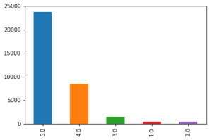
Graphs are powerful and at this point, just by looking at the above bar graph we can conclude that most people are somehow satisfied with the products offered at Amazon. The reason I am saying ‘at’ Amazon is because it is just a platform where anyone can sell their products and the user are giving ratings to the product and not to Amazon. However, if the user is satisfied with the products it also means that Amazon has a lower return rate and lower fraud case (from seller side). The job of a Data Scientist relies not only on how good a model is but also on how useful it is for the business and that’s why these business insights are really important.

Data pre-processing for textual variables

Lowercasing

Before we move forward to calculate the sentiment scores for each review it is important to pre-process the textual data. Lowercasing helps in the process of normalization which is an important step to keep the words in a uniform manner (Welbers, et al., 2017, pp. 245-265).

## Change the reviews type to string
df['reviews.text'] = df['reviews.text'].astype(str)

## Before lowercasing 
df['reviews.text'][2]
'Inexpensive tablet for him to use and learn on, step up from the NABI. He was thrilled with it, learn how to Skype on it 
already...'

## Lowercase all reviews
df['reviews.text'] = df['reviews.text'].apply(lambda x: " ".join(x.lower() for x in x.split()))
df['reviews.text'][2] ## to see the difference
'inexpensive tablet for him to use and learn on, step up from the nabi. he was thrilled with it, learn how to skype on it 
already...'

Special characters

Special characters are non-alphabetic and non-numeric values such as {!,@#$%^ *()~;:/<>|+_-[]?}. Dealing with numbers is straightforward but special characters can be sometimes tricky. During tokenization, special characters create their own tokens and again not helpful for any algorithm, likewise, numbers.

## remove punctuation
df['reviews.text'] = df['reviews.text'].str.replace('[^ws]','')
df['reviews.text'][2]
'inexpensive tablet for him to use and learn on step up from the nabi he was thrilled with it learn how to skype on it already'

Stopwords

Stop-words being most commonly used in the English language; however, these words have no predictive power in reality. Words such as I, me, myself, he, she, they, our, mine, you, yours etc.

stop = stopwords.words('english')
df['reviews.text'] = df['reviews.text'].apply(lambda x: " ".join(x for x in x.split() if x not in stop))
df['reviews.text'][2]
'inexpensive tablet use learn step nabi thrilled learn skype already'

Stemming

Stemming algorithm is very useful in the field of text mining and helps to gain relevant information as it reduces all words with the same roots to a common form by removing suffixes such as -action, ing, -es and -ses. However, there can be problematic where there are spelling errors.

st = PorterStemmer()
df['reviews.text'] = df['reviews.text'].apply(lambda x: " ".join([st.stem(word) for word in x.split()]))
df['reviews.text'][2]
'inexpens tablet use learn step nabi thrill learn skype alreadi'

This step is extremely useful for pre-processing textual data but it also depends on your goal. Here our goal is to calculate sentiment scores and if you look closely to the above code words like ‘inexpensive’ and ‘thrilled’ became ‘inexpens’ and ‘thrill’ after applying this technique. This will help us in text classification to deal with the curse of dimensionality but to calculate the sentiment score this process is not useful.

Sentiment Score

It is now time to calculate sentiment scores of each review and check how these scores look like.

## Define a function which can be applied to calculate the score for the whole dataset

def senti(x):
    return TextBlob(x).sentiment  

df['senti_score'] = df['reviews.text'].apply(senti)

df.senti_score.head()

0                                   (0.3, 0.8)
1                                (0.65, 0.675)
2                                   (0.0, 0.0)
3    (0.29545454545454547, 0.6492424242424243)
4                    (0.5, 0.5827777777777777)
Name: senti_score, dtype: object

As it can be observed there are two scores: the first score is sentiment polarity which tells if the sentiment is positive or negative and the second score is subjectivity score to tell how subjective is the text. The whole code is available here.

In my next article, we will extend this analysis by creating labels based on these scores and finally we will train a classification model.

Deep Learning and Human Intelligence – Part 2 of 2

Data dependency is one of the biggest problem of Deep Learning Architectures. This difficulty lies not so much in the algorithm of Deep Learning as in the invisible structure of the data itself.

This is part 2 of 2 of the Article Series: Deep Learning and Human Intelligence.

We saw that the process of discovering numbers was accompanied with many aspects of what are today basic ideas of Machine Learning. But let us go back, a little before that time, when humankind did not fully discovered the concept of numbers. How would a person, at such a time, perceive quantity and the count of things? Some structures are easily recognizable as patterns of objects, that is numbers, like one sun, 2 trees, 3 children, 4 clouds and so on. Sets of objects are much simpler to count if all the objects of the set are present. In such a case it is sufficient to keep a one-to-one relationship between two different set, without the need for numbers, to make a judgement of crucial importance. One could consider the case of two enemies that go to war and wish to know which has a larger army. It is enough to associate a small stone to every enemy soldier and do the same with his one soldier to be able to decide, depending if stones are left or not, if his army is larger or not, without ever needing to know the exact number soldier of any of the armies.

But also does things can be counted which are not directly visible, and do not allow a direct association with direct observable objects that can be seen, like stones. Would a person, at that time, be able to observe easily the 4-th day since today, 5 weeks from now, when even the concept of week is already composite? Counting in this case is only possible if numbers are already developed through direct observation, and we use something similar with stones in our mind, i.e. a cognitive association, a number. Only then, one can think of the concept of measuring at equidistant moments in time at all. This is the reason why such measurements where still cutting edge in the time of Galileo Galilei as we seen before. It is easily to assume that even in the time when humans started to count, such indirect concepts of numbers were not considered to be in relation with numbers. This implies that many concepts with which we are today accustomed to regard as a number, were considered as belonging to different groups, cluster which are not related. Such an hypothesis is not even that much farfetched. Evidence for such a time are still present in some languages, like Japanese.

When we think of numbers, we associate them with the Indo-Arabic numbers, but in Japanese numbers have no decimal structure and counting depends not only on the length of the set (which is usually considered as the number), but also on the objects that make up the set. In Japanese one can speak of meeting roku people, visiting muttsu cities and seeing ropa birds, but referring each time to the same number: six. Additional, many regular or irregular suffixes make the whole system quite complicated. The division of counting into so many clusters seems unnecessarily complicated today, but can easily be understood from a point of view where language and numbers still form and, the numbers, were not yet a uniform concept. What one can learn from this is that the lack of a unifying concept implies an overly complex dependence on data, which is the present case for Deep Learning and AI in general.

Although Deep Learning was a breakthrough in the development of Artificial Intelligence, the task such algorithms can perform were and remained very narrow. It may identify birds or cancer cells, but it will miss the song of the birds or the cry of the patient with cancer. When Watson, a Deep Learning Architecture played the famous Jeopardy game against two former Champions and won, it still made several simple mistakes, like going for the same wrong answer like the player before. If it could listen to the answer of the candidate, it could delete the top answer it had, and gibe the second which was the right one. With other words, Deep Learning Architecture are not multi-tasking and it is for this reason that some experts in AI are calling them intelligent idiots.

Imagine spending time learning to play a game for years and years, and then, when mastering it and wish to play a different game, to be unable to use any of the past experience (of gaming) for the new one and needing to learn everything from scratch. That could be quite depressing and would make life needlessly difficult. This is the reason why people involved in developing Deep Learning worked from early on in the development of multi-tasking Deep Learning Architectures. On the way a different method of using Deep Learning was discovered: transfer learning. Because the time it takes for a Deep Learning Architecture to learn is very long, transfer learning uses already learned Deep Learning Architectures but for slightly different task. It is similar to the use of past experiences in solving new problems, but, the advantage of transfer learning is, it allow the using of past experiences (what it already learned) which reduces dramatically the amount of new data needed in performing a new task. Still, transfer learning is far away from permitting Deep Learning Architectures to perform any kind of task learning only from one master data set.

The management of a unique master data set which includes all the needed data to enable human accuracy for any human activity, is not enough. One needs another ingredient, the so called cost function which translates, in this case, to the human brain. There are all our experiences and knowledge. How long does it takes to collect sufficient of both to handle a normal human life? How much to achieve our highest potential? If not a lifetime, at least decades. And this also applies to our job: as a IT-developer, a Data Scientist or a professor at the university. We will always have to learn new things, how to use them, and how to expand the limits of our perceptions. The vast amount of information that science has gathered over the last four centuries makes it impossible for any human being to become an expert in all of it. Thus, one has to specialized. After the university, anyone has to choose o subject which is appealing enough to study it for decades. Here is the first sign of what can be understood as data segmentation and dependency. Such improvements can come in various forms: an algorithm in the IT, a theorem in mathematics, a new way to look at particles in physics or a new method to scan for diseases in biology, and so on. But there is a price to pay for specialization: the inability to be an expert in another field or subfield. (Subfields induces limitation!)

Lets take the Deep Learning algorithm itself as an example. For IT and much of everyday life, this is a real breakthrough, but it lacks any scientific, that is mathematical, foundation. There are no theorems which proofs that it will find (converge, to use a mathematical term) the global optimum. This does not appear to be of any great consequences if it can be so efficient, except that, when adding new data and let the algorithm learn the same architecture again, there is no guaranty what so ever that it will be as good as the old model, or even better. On the contrary, it is as real as the efficiency of the first model, that chances are that the new model with the new data will perform worse than the old model, and one has to invest again time in finding a better model, or even a different architecture. On the other hand, with a mathematical proof of convergence, it would be always possible to know in what condition such a convergence can be achieved. In other words, without deep knowledge in mathematics, any proof of a consistent Deep Learning Algorithm is impossible.

Such a situation is true for any other corssover between fields. A mathematical genius will make a lousy biologist, a great chemist will make a average economist, and a top economist will be a poor physicist. Knowledge is difficult to transfer and this is true also for everyday experiences. We learn from very small to play a game like football, but are unable to use the reflexes to play basketball, or tennis better than a normal beginner. We learn a new language after years and years of practice, but are unable to use the way we learned to learn faster other languages. We are trapped within the knowledge we developed from the data we used. It is for this reason why we cannot transfer the knowledge a mathematician has developed over decades to use it in biology or psychology, even if the knowledge is very advanced. Instead of thinking in knowledge, we thing in data. This is similar to the people which were unaware of numbers, and used sets (data) to work with them. Numbers could be very difficult to transmit from one person to another in former times.

Only think on all the great achievements that our society managed, like relativity, quantum mechanics, DNA, machines, etc. Such discoveries are the essences of human knowledge and took millennia to form and centuries to crystalize. Still, all this knowledge is captive in the data, in the special frame in which it was discovered and never had the chance to escape. Imagine the possibility to use thoughts/causalities like the one in relativity or quantum mechanics in biology, or history, or of the concept of DNA in mathematics or art. Imagine a music composition where the law of the notes allows a “tunnel effect” like in quantum mechanics, lower notes to warp the music scales like in relativity and/or to twist two music scale in a helix-like play. How many way to experience life awaits us. Or think of the knowledge hidden in mathematics which could help develop new medicine, but can not be transmitted.

Another example of the connection we experience between knowledge and the data through which we obtain it, are children. They are classical example when it come determine if one is up to explain to them something. Take as an explain something simple they can observe often, like lightning and thunder. Normal concepts like particles, charge, waves, propagation, medium of propagation, etc. become so complicated to expose by other means then the one through which they were discovered, that it becomes nearly impossible to explain to children how it works and that they do not need to fear it. Still, one can use analogy (i.e., transfer) to enable an explanation. Instead of particles, one can use balls, for charge one can use hardness, waves can be shown with strings by keeping one end fix and waving the other, propagation is the movement of the waves from one end of the string to the other end, medium of propagation is the difference between walking in air and water, etc. Although difficult, analogies can be found which enables us to explain even to children how complex phenomena works.

The same is true also for Deep Learning. The model, the knowledge it can extract from the data can be expressed only by such data alone. There is no transformation of the knowledge from one type of data to another. If such a transformation would exists, then Deep Learning would be able to learn any human task by only a set of data, a master data set. Without such a master data set and a corresponding cost function it will be nearly impossible to develop AI that mimics human behavior. With other words, without the realization how our mind works, and how to crystalize by this the data needed, AI will still need to look at all the activities separately. It also implies that AI are restricted to the human understanding of reality and themselves. Only with such a characteristic of a living being, thus also AI, can development of its on occur.

How To Remotely Send R and Python Execution to SQL Server from Jupyter Notebooks

Introduction

Did you know that you can execute R and Python code remotely in SQL Server from Jupyter Notebooks or any IDE? Machine Learning Services in SQL Server eliminates the need to move data around. Instead of transferring large and sensitive data over the network or losing accuracy on ML training with sample csv files, you can have your R/Python code execute within your database. You can work in Jupyter Notebooks, RStudio, PyCharm, VSCode, Visual Studio, wherever you want, and then send function execution to SQL Server bringing intelligence to where your data lives.

This tutorial will show you an example of how you can send your python code from Juptyter notebooks to execute within SQL Server. The same principles apply to R and any other IDE as well. If you prefer to learn through videos, this tutorial is also published on YouTube here:


Environment Setup Prerequisites

  1. Install ML Services on SQL Server

In order for R or Python to execute within SQL, you first need the Machine Learning Services feature installed and configured. See this how-to guide.

  1. Install RevoscalePy via Microsoft’s Python Client

In order to send Python execution to SQL from Jupyter Notebooks, you need to use Microsoft’s RevoscalePy package. To get RevoscalePy, download and install Microsoft’s ML Services Python Client. Documentation Page or Direct Download Link (for Windows).

After downloading, open powershell as an administrator and navigate to the download folder. Start the installation with this command (feel free to customize the install folder): .\Install-PyForMLS.ps1 -InstallFolder “C:\Program Files\MicrosoftPythonClient”

Be patient while the installation can take a little while. Once installed navigate to the new path you installed in. Let’s make an empty folder and open Jupyter Notebooks: mkdir JupyterNotebooks; cd JupyterNotebooks; ..\Scripts\jupyter-notebook

Create a new notebook with the Python 3 interpreter:


To test if everything is setup, import revoscalepy in the first cell and execute. If there are no error messages you are ready to move forward.

Database Setup (Required for this tutorial only)

For the rest of the tutorial you can clone this Jupyter Notebook from Github if you don’t want to copy paste all of the code. This database setup is a one time step to ensure you have the same data as this tutorial. You don’t need to perform any of these setup steps to use your own data.

  1. Create a database

Modify the connection string for your server and use pyodbc to create a new database.

import pyodbc  
# creating a new db to load Iris sample in 
new_db_name = "MLRemoteExec" connection_string = "Driver=SQL Server;Server=localhost\MSSQLSERVER2017;Database={0};Trusted_Connection=Yes;" 

cnxn = pyodbc.connect(connection_string.format("master"), autocommit=True) 

cnxn.cursor().execute("IF EXISTS(SELECT * FROM sys.databases WHERE [name] = '{0}') DROP DATABASE {0}".format(new_db_name)) 

cnxn.cursor().execute("CREATE DATABASE " + new_db_name)

cnxn.close()

print("Database created") 
  1. Import Iris sample from SkLearn

Iris is a popular dataset for beginner data science tutorials. It is included by default in sklearn package.

from sklearn import datasetsimport pandas as pd
# SkLearn has the Iris sample dataset built in to the packageiris = datasets.load_iris()
df = pd.DataFrame(iris.data, columns=iris.feature_names)
  1. Use RecoscalePy APIs to create a table and load the Iris data

(You can also do this with pyodbc, sqlalchemy or other packages)

from revoscalepy import RxSqlServerData, rx_data_step
# Example of using RX APIs to load data into SQL table. You can also do this with pyodbc
table_ref = RxSqlServerData(connection_string=connection_string.format(new_db_name), table="Iris")rx_data_step(input_data = df, output_file = table_ref, overwrite = True)print("New Table Created: Iris")
print("Sklearn Iris sample loaded into Iris table")

Define a Function to Send to SQL Server

Write any python code you want to execute in SQL. In this example we are creating a scatter matrix on the iris dataset and only returning the bytestream of the .png back to Jupyter Notebooks to render on our client.

def send_this_func_to_sql():
    from revoscalepy import RxSqlServerData, rx_import
    from pandas.tools.plotting import scatter_matrix
    import matplotlib.pyplot as plt
    import io    
# remember the scope of the variables in this func are within our SQL Server Python Runtime
    connection_string = "Driver=SQL Server;Server=localhost\MSSQLSERVER2017; Database=MLRemoteExec;Trusted_Connection=Yes;"

# specify a query and load into pandas dataframe df
    sql_query = RxSqlServerData(connection_string=connection_string, sql_query = "select * from Iris")

    df = rx_import(sql_query)
    scatter_matrix(df)

# return bytestream of image created by scatter_matrix
    buf = io.BytesIO()
    plt.savefig(buf, format="png")
    buf.seek(0)
    return buf.getvalue()

Send execution to SQL

Now that we are finally set up, check out how easy sending remote execution really is! First, import revoscalepy. Create a sql_compute_context, and then send the execution of any function seamlessly to SQL Server with RxExec. No raw data had to be transferred from SQL to the Jupyter Notebook. All computation happened within the database and only the image file was returned to be displayed.

from IPython import display
import matplotlib.pyplot as plt 
from revoscalepy import RxInSqlServer, rx_exec# create a remote compute context with connection to SQL Server

sql_compute_context = RxInSqlServer(connection_string=connection_string.format(new_db_name))

# use rx_exec to send the function execution to SQL Server

image = rx_exec(send_this_func_to_sql, compute_context=sql_compute_context)[0]

# only an image was returned to my jupyter client. All data remained secure and was manipulated in my db.

display.Image(data=image)

While this example is trivial with the Iris dataset, imagine the additional scale, performance, and security capabilities that you now unlocked. You can use any of the latest open source R/Python packages to build Deep Learning and AI applications on large amounts of data in SQL Server. We also offer leading edge, high-performance algorithms in Microsoft’s RevoScaleR and RevoScalePy APIs. Using these with the latest innovations in the open source world allows you to bring unparalleled selection, performance, and scale to your applications.

Learn More

Check out SQL Machine Learning Services Documentation to learn how you can easily deploy your R/Python code with SQL stored procedures making them accessible in your ETL processes or to any application. Train and store machine learning models in your database bringing intelligence to where your data lives.

Other YouTube Tutorials:

Interview – The Importance of Machine Learning for the Data Driven Business

To become more data-driven, organizations must mature their analytics and automate more of their decision making processes for innovation and differentiation. Data science seems like the right approach, yet is a new and fast moving field that seems to have as many dead ends as it has high ways to value. Cloudera Fast Forward Labs, led by Hilary Mason, shows companies the way.

Alice Albrecht is a research engineer at Cloudera Fast Forward Labs.  She spends her days researching the latest and greatest in machine learning and artificial intelligence and bringing that knowledge to working prototypes and delivering concrete advice for clients.  Prior to joining Fast Forward Labs, Alice worked in both finance and technology companies as a practicing data scientist, data science leader, and – most recently – a data product manager.  In addition to teaching machines to do cool things, Alice is passionate about mentoring and helping others grow in their careers.  Alice holds a PhD from Yale in cognitive neuroscience where she studied how humans summarize sensory information from the world around them and the neural substrates that underlie those summaries.

Read this article in German:
“Interview – Die Bedeutung von Machine Learning für das Data Driven Business“

Data Science Blog: Ms. Albrecht, you are a well-known keynote speaker for data science and artificial intelligence. While data science has arrived business already, deep learning seems to be the new trend. Is artificial intelligence for business already normal business or is it an overrated hype?

I’d say it isn’t either of those two options.  Data science is now widely adopted but companies still struggle to integrate this new discipline into their existing businesses.  As for deep learning, it really depends on the company that’s looking into using this technique.  I wouldn’t say that deep learning is by any means part of business as usual- nor should it be.  It’s a tool like any other and building a capacity for using a tool without clearly defined business needs is a recipe for disaster.

Data Science Blog: Just to make sure what we are talking about: What are the differences and overlaps between data analytics, data science, machine learning, deep learning and artificial intelligence?

Here at Cloudera Fast Forward Labs, we like to think of data analytics as collecting data and counting things (mostly for quick charts and reports).  Data science solves business problems by counting cleverly and predicting things with the data that’s collected.  Machine learning is about solving problems with new kinds of feedback loops that improve with more data.  Deep learning is a particular type of machine learning and is not itself a separate concept or type of tool.  Artificial intelligence taps into something more complicated than what we’re seeing today – it’s much broader than training machines to repetitively do very specialized tasks or solve very narrow problems.

Data Science Blog: And how can we add the context to big data?

From a theoretical perspective, data science has been around for decades. The building blocks for modern day machine learning, deep learning and artificial intelligence are based on mathematical theorems  that go back to the 1940’s and 1950’s. The challenge was that at the time, compute power and data storage capacity were simply too expensive for the approaches to be implemented. Today that’s all changed.. Not only has the cost of data storage dropped considerably, open source technology like Apache Hadoop has made it possible to store any volume of data at costs approaching zero. Compute power, even highly specialised chip architectures, are now also available on demand and only for the time organisations need them through public and private cloud solutions. The decreased cost of both data storage and compute power, together with a growing list of tools and resources readily available via the open source community allows companies of any size to benefit from data (no matter that size of that data).

Data Science Blog: What are the challenges for organizations in getting started with data science?

I see two big challenges when getting started with data science.  One is ensuring that you have organizational alignment around exactly what type of work data scientists will deliver (and timing for those projects).  The second hurdle is around ensuring that you have the right data in place before you start hiring data scientists. This can be tricky if you don’t have in-house expertise in this area, so sometimes it’s better to hire a data engineer or a data strategist (or director of data science) before you ever get started building out a data science team.

Data Science Blog: There are many discussions about how to build a data-driven business. Is it just about using data science to get a better understanding of customer behavior?

No, being data driven doesn’t just mean better understanding your customers (though that is one way that data science can help in an organization).  Aside from building an organization that relies on data and analytics to help them make decisions (about customer behavior or otherwise), being a data-driven business means that data is powering your core products.

Data Science Blog: The number of technologies, tools and frameworks is increasing. For organizations this also means increasing complexity. Do companies need to stay always up-to-date or could it be an advice to wait and imitate pioneers later?

While it’s not critical (or advisable) for organizations to adopt every new advancement that comes along, it is critical for them to stay abreast of emerging frameworks.  If a business waits to see what others are doing, and therefore don’t invest in understanding how new advancements can affect their particular business, they’ve likely already missed the boat.

Data Science Blog: Global players have big budgets just for doing research and setting up data labs. Middle-sized companies need to see the break even point soon. How can we accelerate the value generation of data science?

Having a team that is highly focused on a specific set of projects that are well-scoped and aligned to the business makes all the difference.  Data science and machine learning don’t have to sacrifice doing research and being innovative in order to produce value.  The biggest difference is that smaller teams will have to be more aware of how their choice of project fits into emerging frameworks and their particular acute and near term business needs.

Data Science Blog: How does Cloudera Fast Forward Labs help other organizations to accelerate their start with machine learning?

We advise organizations, based on their particular needs, on what the latest advancements are in machine learning and data science, how to build and structure their data teams to develop the capabilities they need to meet their goals, and how to quickly implement custom forward-looking solutions using their own data and in-house expertise.

Data Science Blog: Finally, a question for our younger readers who are looking for a career as a data expert: What makes a good data scientist? Do you like to work with introverted coding nerds or the data loving business experts?

A good data scientists should be deeply curious and have a love for the ways in which data can lead to new discoveries and power the next generation of products.  We expect the people who thrive in this field to come from a variety of backgrounds and experiences.

Deep Learning and Human Intelligence – Part 1 of 2

Many people are under the impression that the new wave of data science, machine learning and/or digitalization is new, that it did not exist before. But its history is as long as the history of humanity and/or science itself.  The scientific discovery could hardly take place without the necessary data. Even the process of discovering the numbers included elements of machine learning: pattern recognition, comparison between different groups (ranking), clustering, etc. So what differentiates mathematical formulas from machine learning and how does it relate to artificial intelligence?

There is no difference between the two if seen from the perspective of formulas however, such a perspective limits the type of data to which they can be applied. Data stored via tables consist of structured data and are stored in so-called relational databases. The reason for such a data storage is the connection between different fields that assume a well-established structure in advance, such as a company’s sales or balance sheet. However, with the emergence of personal computers, many of the daily activities have been digitalized: music, pictures, movies, and so on. All this information is stored unrelated to other data and therefore called unstructured data.

IEEE International Conference on Computer Vision (ICCV), 2015, DOI: 10.1109/ICCV.2015.428

Copyright: IEEE International Conference on Computer Vision (ICCV), 2015, DOI: 10.1109/ICCV.2015.428

The essence of scientific discoveries was and will be structure. Not surprisingly, the mathematical formulas revolve around relations between variables – information, in general. For example, Galileo derived the law of falling balls from measuring the successive hight of a falling ball. The main difficulty was to obtain measurements at regular time intervals. What about if the data is not structured, which mathematical formula should be applied then? There is a distribution of people’s height, but no distribution for the pictures taken in all holidays for the last year, there is an amplitude for acoustic signals, but no function that detects the similarity between two songs. This is one of the reasons why machine learning focuses heavily on clustering and classification.

Roughly speaking, these simple examples are enough to categorize the difference between scientific discovery and machine learning. Science is about discovering relationships between different variables, Machine Learning tries to automatize processes. Every technical improvement is part of the automation, so why is everything different in this case? Because the current automation deals with human intelligence. The car automates the walking, the kitchen stove the fire, but Machine Learning parts of the human intelligence. There is a difference between the previous automation steps and those of human intelligence. All the previous ones are either outside the human body – such as Fire – or unconsciously executed (once learned) – walking, spinning, etc. The automation induced by Machine Learning affects a part of the human intelligence that we consciously perceive. Of course, today’s machine learning tools are unable to automate all human intelligence, but it is a fascinating step in that direction.

A breakthrough in Machine Learning tasks was achieved in 2012 when the first Deep Learning algorithm for detecting types of images, reached near-human accuracy. It could appreciate the likelihood that the image is a human face, a train, a ball or a fish without having “seen” the picture before. Such an algorithm can be used in various areas:  personally – facial recognition in pictures and/or social media – as tagging of images or videos, medicine – cancer detection, etc. For understanding such cutting-edge issues of classification, one cannot avoid understanding how Deep Learning works. To see the beauty of such algorithms and, at the same time, to be able to comprehend the difficulty of working with them, an example will be the best guide.

The building blocks of Deep Learning are neurons, operational units, which perform mathematical operations or logical operations like AND, OR, etc., and are modelled after the neurons in the brain. Already in the 1950’s two neuroscientist, Hubel and Wiesel, observed that not all neurons in the brain are responding in the same fashion to visual stimuli. Some responded only to horizontal lines, whereas others to vertical lines, with other words, the brain is constructed with specialized neurons. Groups of such neurons are called, in the Machine Learning community, layers. Like in the brain, neurons with different properties are clustered in different layers. This implies that layers have also specific properties and have to be arranged in a specific way, called architecture. It is this architecture which differentiates Deep Learning from Artificial Neuronal Networks (ANN are similar to a layer).

Unfortunately, scientists still haven’t figured out how the brain works, thus to discover how to train Deep Learning from data was not an easy task, and is also the reason why another example is used to explain the training of Deep Learning: the eye. One has always to remember: once it is known how Deep Learning works, it is simple to find example which illustrates the working mechanism.  For such an analogy, it is sufficient for someone without any knowledge about Deep Learning, to keep in mind only the elements that compose such architectures: input data, different layers of neurons, output layers, ReLu’s.

Input data are any type of information, in our example it is light. Of course, that Deep Learning is not limited only to images or videos, but also to sound and/or time series, which would imply that the example would be the ear and sound waves, or the brain and numbers.

Layers can be seen as cells in the eye. It is well known that the eye is formed of different layers connected to each other with each of them having different properties, functionalities. The same is true also for the layers of a Deep Learning architecture: one can see the neurons as cells of the layer as the tissue. While, mathematically, the neurons are nothing more than simple operations, usually linear weight functions, they can be seen as the properties of individual cells. Each layer has one weight matrix, which gives the neuron (and layer) specific properties depending on the data and the task at hand.

It is here that the architecture becomes very important. What Deep Learning offers is a default setting of the layers with unknown weights. One can see this as trying to build an eye knowing that there are different types of cells and different ways how tissues of such cells can be arranged, but not which cell exactly is needed (with what properties) and which arrangement of layers works best. Such an approach has the advantage that one is capable of building any type of organ desired, but the disadvantage is also very obvious: it is time consuming to find the appropriate cell properties and layers arrangements.

Still, the strategy of Deep Learning is a significant departure from the Machine Learning approaches. The performance of Machine Learning methods is as good as the features engineering performed by Data Scientists, and thus depending on the creativity of the Data Scientist. In the case of Deep Learning the engineers of the features is performed automatically as part of the model building. This is a huge improvement, as the only difficult task is to have enough data and computer power to find the right weights matrices. Such an endeavor was performed also by nature for the eye — and is also the reason why one can choose it as an example for Deep Learning — evolution. It is not surprising that Deep Learning is one of the best direction scientists have of Artificial Intelligence today.

The evolution of the eye can be seen, from the perspective of Data Scientists, as the continuous training of a Deep Learning architecture which enables to recognize and track one or more objects. The performance of the evolutional process can be summed up as the fine tuning of the cells which are getting more and more susceptible to light and the adaptation of layers to enable a better vision. Different animals in different environments and different targets — as the hawk and the fly — developed different eyes than humans, but they all work according to the same principle. The tasks that Deep Learning is performing today are similar, for example it can be used to drive cars but there is still a difference:  there is no connection to other organs. Deep Learning is not the approximation of an Artificial Organism, like an android, but a simplified Artificial Organ that can work on its own.

Returning to the working mechanism of the Deep Learning architecture, we can already follow the analogy of what happens if a ray of light is hitting the eye. Once the eye is fully adapted to the task, one can followed how the information enters the Deep Learning architecture (Artificial Eye) by penetrating the input layer. already here arises the question, what kind of eye is the best? One where a small source of light can reach as many neurons as possible, or the one where the light sources reaches only few neurons? In order to take such a decision, a last piece of the puzzle is required: ReLu. One can see them as synapses between neurons (cells) and/or similarly for tissue. By using continuous functions, such as the shape of the latter ‘S’ (called sigmoid), the information from one neuron will be distributed over a large number of other neurons. If one uses the maximum function, then only few neurons are updated with processed information from earlier layers.

Such sparse structures between neurons, was a major improvement in the development of the technique of training Deep Learning architectures. Again, it has a strong evolutionary analogy: energy efficiency. By needing less neurons, the tissues and architecture are both kept to a minimal size which enables flexibility in development and less energy. As the information is process by the different layers, the Artificial Eye is gathering more and more complex (non-linear) structures — the adapted features –, which help to decide, from past experience, what kind of object is detected.

This was part 1 of 2 of the article series. Continue with Part 2.

Bringing intelligence to where data lives: Python & R embedded in T-SQL

Introduction

Did you know that you can write R and Python code within your T-SQL statements? Machine Learning Services in SQL Server eliminates the need for data movement. Instead of transferring large and sensitive data over the network or losing accuracy with sample csv files, you can have your R/Python code execute within your database. Easily deploy your R/Python code with SQL stored procedures making them accessible in your ETL processes or to any application. Train and store machine learning models in your database bringing intelligence to where your data lives.

You can install and run any of the latest open source R/Python packages to build Deep Learning and AI applications on large amounts of data in SQL Server. We also offer leading edge, high-performance algorithms in Microsoft’s RevoScaleR and RevoScalePy APIs. Using these with the latest innovations in the open source world allows you to bring unparalleled selection, performance, and scale to your applications.

If you are excited to try out SQL Server Machine Learning Services, check out the hands on tutorial below. If you do not have Machine Learning Services installed in SQL Server,you will first want to follow the getting started tutorial I published here: 

How-To Tutorial

In this tutorial, I will cover the basics of how to Execute R and Python in T-SQL statements. If you prefer learning through videos, I also published the tutorial on YouTube.

Basics

Open up SQL Server Management Studio and make a connection to your server. Open a new query and paste this basic example: (While I use Python in these samples, you can do everything with R as well)

EXEC sp_execute_external_script @language = N'Python',
@script = N'print(3+4)'

Sp_execute_external_script is a special system stored procedure that enables R and Python execution in SQL Server. There is a “language” parameter that allows us to choose between Python and R. There is a “script” parameter where we can paste R or Python code. If you do not see an output print 7, go back and review the setup steps in this article.

Parameter Introduction

Now that we discussed a basic example, let’s start adding more pieces:

EXEC sp_execute_external_script  @language =N'Python', 
@script = N' 
OutputDataSet = InputDataSet;
',
@input_data_1 =N'SELECT 1 AS Col1';

Machine Learning Services provides more natural communications between SQL and R/Python with an input data parameter that accepts any SQL query. The input parameter name is called “input_data_1”.
You can see in the python code that there are default variables defined to pass data between Python and SQL. The default variable names are “OutputDataSet” and “InputDataSet” You can change these default names like this example:

EXEC sp_execute_external_script  @language =N'Python', 
@script = N' 
MyOutput = MyInput;
',
@input_data_1_name = N'MyInput',
@input_data_1 =N'SELECT 1 AS foo',
@output_data_1_name =N'MyOutput';

As you executed these examples, you might have noticed that they each return a result with “(No column name)”? You can specify a name for the columns that are returned by adding the WITH RESULT SETS clause to the end of the statement which is a comma separated list of columns and their datatypes.

EXEC sp_execute_external_script  @language =N'Python', 
@script=N' 
MyOutput = MyInput;
',
@input_data_1_name = N'MyInput',
@input_data_1 =N'
SELECT 1 AS foo,
2 AS bar
',
@output_data_1_name =N'MyOutput'
WITH RESULT SETS ((MyColName int, MyColName2 int));

Input/Output Data Types

Alright, let’s discuss a little more about the input/output data types used between SQL and Python. Your input SQL SELECT statement passes a “Dataframe” to python relying on the Python Pandas package. Your output from Python back to SQL also needs to be in a Pandas Dataframe object. If you need to convert scalar values into a dataframe here is an example:

EXEC sp_execute_external_script  @language =N'Python', 
@script=N' 
import pandas as pd
c = 1/2
d = 1*2
s = pd.Series([c,d])
df = pd.DataFrame(s)
OutputDataSet = df
'

Variables c and d are both scalar values, which you can add to a pandas Series if you like, and then convert them to a pandas dataframe. This one shows a little bit more complicated example, go read up on the python pandas package documentation for more details and examples:

EXEC sp_execute_external_script  @language =N'Python', 
@script=N' 
import pandas as pd
s = {"col1": [1, 2], "col2": [3, 4]}
df = pd.DataFrame(s)
OutputDataSet = df
'

You now know the basics to execute Python in T-SQL!

Did you know you can also write your R and Python code in your favorite IDE like RStudio and Jupyter Notebooks and then remotely send the execution of that code to SQL Server? Check out these documentation links to learn more: https://aka.ms/R-RemoteSQLExecution https://aka.ms/PythonRemoteSQLExecution

Check out the SQL Server Machine Learning Services documentation page for more documentation, samples, and solutions. Check out these E2E tutorials on github as well.

Would love to hear from you! Leave a comment below to ask a question, or start a discussion!

Applying Data Science Techniques in Python to Evaluate Ionospheric Perturbations from Earthquakes

Multi-GNSS (Galileo, GPS, and GLONASS) Vertical Total Electron Content Estimates: Applying Data Science techniques in Python to Evaluate Ionospheric Perturbations from Earthquakes

1 Introduction

Today, Global Navigation Satellite System (GNSS) observations are routinely used to study the physical processes that occur within the Earth’s upper atmosphere. Due to the experienced satellite signal propagation effects the total electron content (TEC) in the ionosphere can be estimated and the derived Global Ionosphere Maps (GIMs) provide an important contribution to monitoring space weather. While large TEC variations are mainly associated with solar activity, small ionospheric perturbations can also be induced by physical processes such as acoustic, gravity and Rayleigh waves, often generated by large earthquakes.

In this study Ionospheric perturbations caused by four earthquake events have been observed and are subsequently used as case studies in order to validate an in-house software developed using the Python programming language. The Python libraries primarily utlised are Pandas, Scikit-Learn, Matplotlib, SciPy, NumPy, Basemap, and ObsPy. A combination of Machine Learning and Data Analysis techniques have been applied. This in-house software can parse both receiver independent exchange format (RINEX) versions 2 and 3 raw data, with particular emphasis on multi-GNSS observables from GPS, GLONASS and Galileo. BDS (BeiDou) compatibility is to be added in the near future.

Several case studies focus on four recent earthquakes measuring above a moment magnitude (MW) of 7.0 and include: the 11 March 2011 MW 9.1 Tohoku, Japan, earthquake that also generated a tsunami; the 17 November 2013 MW 7.8 South Scotia Ridge Transform (SSRT), Scotia Sea earthquake; the 19 August 2016 MW 7.4 North Scotia Ridge Transform (NSRT) earthquake; and the 13 November 2016 MW 7.8 Kaikoura, New Zealand, earthquake.

Ionospheric disturbances generated by all four earthquakes have been observed by looking at the estimated vertical TEC (VTEC) and residual VTEC values. The results generated from these case studies are similar to those of published studies and validate the integrity of the in-house software.

2 Data Cleaning and Data Processing Methodology

Determining the absolute VTEC values are useful in order to understand the background ionospheric conditions when looking at the TEC perturbations, however small-scale variations in electron density are of primary interest. Quality checking processed GNSS data, applying carrier phase leveling to the measurements, and comparing the TEC perturbations with a polynomial fit creating residual plots are discussed in this section.

Time delay and phase advance observables can be measured from dual-frequency GNSS receivers to produce TEC data. Using data retrieved from the Center of Orbit Determination in Europe (CODE) site (ftp://ftp.unibe.ch/aiub/CODE), the differential code biases are subtracted from the ionospheric observables.

2.1 Determining VTEC: Thin Shell Mapping Function

The ionospheric shell height, H, used in ionosphere modeling has been open to debate for many years and typically ranges from 300 – 400 km, which corresponds to the maximum electron density within the ionosphere. The mapping function compensates for the increased path length traversed by the signal within the ionosphere. Figure 1 demonstrates the impact of varying the IPP height on the TEC values.

Figure 1 Impact on TEC values from varying IPP heights. The height of the thin shell, H, is increased in 50km increments from 300 to 500 km.

2.2 Phase Smoothing

For dual-frequency GNSS users TEC values can be retrieved with the use of dual-frequency measurements by applying calculations. Calculation of TEC for pseudorange measurements in practice produces a noisy outcome and so the relative phase delay between two carrier frequencies – which produces a more precise representation of TEC fluctuations – is preferred. To circumvent the effect of pseudorange noise on TEC data, GNSS pseudorange measurements can be smoothed by carrier phase measurements, with the use of the carrier phase smoothing technique, which is often referred to as carrier phase leveling.

Figure 2 Phase smoothed code differential delay

2.3 Residual Determination

For the purpose of this study the monitoring of small-scale variations in ionospheric electron density from the ionospheric observables are of particular interest. Longer period variations can be associated with diurnal alterations, and changes in the receiver- satellite elevation angles. In order to remove these longer period variations in the TEC time series as well as to monitor more closely the small-scale variations in ionospheric electron density, a higher-order polynomial is fitted to the TEC time series. This higher-order polynomial fit is then subtracted from the observed TEC values resulting in the residuals. The variation of TEC due to the TID perturbation are thus represented by the residuals. For this report the polynomial order applied was typically greater than 4, and was chosen to emulate the nature of the arc for that particular time series. The order number selected is dependent on the nature of arcs displayed upon calculating the VTEC values after an initial inspection of the VTEC plots.

3 Results

3.1 Tohoku Earthquake

For this particular report, the sampled data focused on what was retrieved from the IGS station, MIZU, located at Mizusawa, Japan. The MIZU site is 39N 08′ 06.61″ and 141E 07′ 58.18″. The location of the data collection site, MIZU, and the earthquake epicenter can be seen in Figure 3.

Figure 3 MIZU IGS station and Tohoku earthquake epicenter [generated using the Python library, Basemap]

Figure 4 displays the ionospheric delay in terms of vertical TEC (VTEC), in units of TECU (1 TECU = 1016 el m-2). The plot is split into two smaller subplots, the upper section displaying the ionospheric delay (VTEC) in units of TECU, the lower displaying the residuals. The vertical grey-dashed lined corresponds to the epoch of the earthquake at 05:46:23 UT (2:46:23 PM local time) on March 11 2011. In the upper section of the plot, the blue line corresponds to the absolute VTEC value calculated from the observations, in this case L1 and L2 on GPS, whereby the carrier phase leveling technique was applied to the data set. The VTEC values are mapped from the STEC values which are calculated from the LOS between MIZU and the GPS satellite PRN18 (on Figure 4 denoted G18). For this particular data set as seen in Figure 4, a polynomial fit of  five degrees was applied, which corresponds to the red-dashed line. As an alternative to polynomial fitting, band-pass filtering can be employed when TEC perturbations are desired. However for the scope of this report polynomial fitting to the time series of TEC data was the only method used. In the lower section of Figure 4 the residuals are plotted. The residuals are simply the phase smoothed delay values (the blue line) minus the polynomial fit line (the red-dashed line). All ionosphere delay plots follow the same layout pattern and all time data is represented in UT (UT = GPS – 15 leap seconds, whereby 15 leap seconds correspond to the amount of leap seconds at the time of the seismic event). The time series shown for the ionosphere delay plots are given in terms of decimal of the hour, so that the format follows hh.hh.

Figure 4 VTEC and residual plot for G18 at MIZU on March 11 2011

3.2 South Georgia Earthquake

In the South Georgia Island region located in the North Scotia Ridge Transform (NSRT) plate boundary between the South American and Scotia plates on 19 August 2016, a magnitude of 7.4 MW earthquake struck at 7:32:22 UT. This subsection analyses the data retrieved from KEPA and KRSA. As well as computing the GPS and GLONASS TEC values, four Galileo satellites (E08, E14, E26, E28) are also analysed. Figure 5 demonstrates the TEC perturbations as computed for the Galileo L1 and L5 carrier frequencies.

Figure 5 VTEC and residual plots at KRSA on 19 August 2016. The plots are from the perspective of the GNSS receiver at KRSA, for four Galileo satellites (a) E08; (b) E14; (c) E24; (d) E26. The y-axes and x-axes in all plots do not conform with one another but are adjusted to fit the data. The y-axes for the residual section of each plot is consistent with one another.

Figure 6 Geometry of the Galileo (E08, E14, E24 and E26) satellites’ projected ground track whereby the IPP is set to 300km altitude. The orange lines correspond to tectonic plate boundaries.

4 Conclusion

The proximity of the MIZU site and magnitude of the Tohoku event has provided a remarkable – albeit a poignant – opportunity to analyse the ocean-ionospheric coupling aftermath of a deep submarine seismic event. The Tohoku event has also enabled the observation of the origin and nature of the TIDs generated by both a major earthquake and tsunami in close proximity to the epicenter. Further, the Python software developed is more than capable of providing this functionality, by drawing on its mathematical packages, such as NumPy, Pandas, SciPy, and Matplotlib, as well as employing the cartographic toolkit provided from the Basemap package, and finally by utilizing the focal mechanism generation library, Obspy.

Pre-seismic cursors have been investigated in the past and strongly advocated in particular by Kosuke Heki. The topic of pre-seismic ionospheric disturbances remains somewhat controversial. A potential future study area could be the utilization of the Python program – along with algorithmic amendments – to verify the existence of this phenomenon. Such work would heavily involve the use of Scikit-Learn in order to ascertain the existence of any pre-cursors.

Finally, the code developed is still retained privately and as of yet not launched to any particular platform, such as GitHub. More detailed information on this report can be obtained here:

Download as PDF

Data Science Modeling and Featurization

Overview

Data modeling is an essential part of the data science pipeline. This, combined with the fact that it is a very rewarding process, makes it the one that often receives the most attention among data science learners. However, things are not as simple as they may seem, since there is much more to it than applying a function from a particular class of a package and applying it on the data available.

A big part of data science modeling involves evaluating a model, for example, making sure that it is robust and therefore reliable. Also, data science modeling is closely linked to creating an information rich feature set. Moreover, it entails a variety of other processes that ensure that the data at hand is harnessed as much as possible.

What Is a Robust Data Model?

When it comes to robust models, worthy of making it to production, these need to tick several boxes. First of all, they need to have a good performance, based on various metrics. Oftentimes a single metric can be misleading, as how well a model performs has many aspects, especially for classification problems.

In addition, a robust model has good generalization. This means that the model performs well for various datasets, not just the one it has been trained on.

Sensitivity analysis is another aspect of a data science modeling, something essential for thoroughly testing a model to ensure it is robust enough. Sensitivity is a condition whereby a model’s output is bound to change significantly if the inputs change even slightly. This is quite undesirable and needs to be checked since a robust model ought to be stable.

Finally, interpretability is an important aspect too, though it’s not always possible. This has to do with how easy it is to interpret a model’s results. Many modern models, however, are more like black boxes, making it particularly difficult to interpret them. Nevertheless, it is often preferable to opt for an interpretable model, especially if we need to defend its outputs to others.

How Is Featurization Accomplished?

In order for a model to maximize its potential, it needs an information rich set of features. The latter can be created in various ways. Whatever the case, cleaning up the data is a prerequisite. This involves removing or correcting problematic data points, filling in missing values wherever possible, and in some cases removing noisy variables.

Before you can use variables in a model, you need to perform normalization on them. This is usually accomplished through a linear transformation ensuring that the variable’s values are around a certain range. Oftentimes, normalization is sufficient for turning your variables into features, once they are cleaned.

Binning is another process that can aid in featurization. This entails creating nominal (discreet) variables, which can in turn be broken down into binary features, to be used in a data model.

Finally, some dimensionality reduction method (e.g. PCA) can be instrumental in shaping up your feature-set. This has to do with creating linear combinations of features, aka meta-features, which express the same information in fewer dimensions.

Some Useful Considerations

Beyond these basic attributes of data science modeling there several more that every data scientist has in mind in order to create something of value from the available data. Things like in-depth testing using sensitivity analysis, specialized sampling, and various aspects of model performance (as well as tweaking the model to optimize for a particular performance metric) are parts of data science modeling that require meticulous study and ample practice. After all, even though this part of data science is fairly easy to pick up, it takes a while to master, while performing well in it is something that every organization can benefit from.

Resources

To delve more into all this, there are various relevant resources you can leverage, helping you in not just the methodologies involved but also in the mindset behind them. Here are two of the most useful ones.

  1. Data Science Modeling Tutorial on the Safari platform
  2. Data Science Mindset, Methodologies and Misconceptions book (Technics Publications)

Process Analytics – Data Analysis for Process Audit & Improvement

Process Mining: Innovative data analysis for process optimization and audit

Step-by-Step: New ways to detect compliance violations with Process Analytics

In the course of the advancing digitization, an enormous upheaval of everyday work is currently taking place to ensure the complete recording of all steps in IT systems. In addition, companies are increasingly confronted with increasingly demanding regulatory requirements on their IT systems.


Read this article in German:
“Process Mining: Innovative Analyse von Datenspuren für Audit und Forensik “


The unstoppable trend towards a connected world will further increase the possibilities of process transparency, but many processes in the company area are already covered by one or more IT systems. Each employee, as well as any automated process, leaves many data traces in IT backend systems, from which processes can be replicated retroactively or in real time. These include both obvious processes, such as the entry of a recorded purchase order or invoice, as well as partially hidden processes, such as the modification of certain entries or deletion of these business objects.

1 Understanding Process Analytics

Process Analytics is a data-driven methodology of the actual process analysis, which originates in forensics. In the wake of the increasing importance of computer crime, it became necessary to identify and analyze the data traces that potential criminals left behind in IT systems in order to reconstruct the event as much as possible.

With the trend towards Big Data Analytics, Process Analytics has not only received new data bases, but has also been further developed as an analytical method. In addition, the visualization enables the analyst or the report recipient to have a deeper understanding of even more complex business processes.

While conventional process analysis primarily involves employee interviews and monitoring of the employees at the desk in order to determine actual processes, Process Analytics is a leading method, which is purely fact-based and thus objectively approaching the processes. It is not the employees who are asked, but the IT systems, which not only store all the business objects recorded in a table-oriented manner, but also all process activities. Every IT system for enterprise purposes log all relevant activities of the whole business process, in the background and invisible to the users, such as orders, invoices or customer orders, with a time stamp.

2 The right choice of the processes to analyze

Today almost every company works with at least one ERP system. As other systems are often used, it is clear which processes can not be analyzed: Those processes, which are still carried out exclusively on paper and in the minds of the employees, which are typical decision-making processes at the strategic level and not logged in IT systems.

Operational processes, however, are generally recorded almost seamlessly in IT systems. Furthermore, almost all operational decisions are recorded by status flags in datasets.

The operational processes, which can be reconstructed and analyzed with Process Mining very well and which are of equal interest from the point of view of compliance, include for example:

– Procurement

– Logistics / Transport

– Sales / Ordering

– Warranty / Claim Management

– Human Resource Management

Process Analytics enables the greatest possible transparency across all business processes, regardless of the sector and the department. Typical case IDs are, for example, sales order number, procurement order number, customer or material numbers.

3 Selection of relevant IT systems

In principle, every IT system used in the company should be examined with regard to the relevance for the process to be analyzed. As a rule, only the ERP system (SAP ERP or others) is relevant for the analysis of the purchasing processes. However, for other process areas there might be other IT systems interesting too, for example separate accounting systems, a CRM or a MES system, which must then also be included.

Occasionally, external data should also be integrated if they provide important process information from externally stored data sources – for example, data from logistics partners.

4 Data Preparation

Before the start of the data-driven process analysis, the data directly or indirectly indicating process activities must be identified, extracted and processed in the data sources. The data are stored in database tables and server logs and are collected via a data warehousing procedure and converted into a process protocol or – also called – event log.

The event log is usually a very large and wide table which, in addition to the actual process activities, also contains parameters which can be used to filter cases and activities. The benefit of this filter option is, for example, to show only process flows where special product groups, prices, quantities, volumes, departments or employee groups are involved.

5 Analysis Execution

The actual inspection is done visually and thus intuitively with an interactive process flow diagram, which represents the actual processes as they could be extracted from the IT systems. The event log generated by the data preparation is loaded into a data visualization software (e.g. Celonis PM Software), which displays this log by using the case IDs and time stamps and transforms this information in a graphical process network. The process flows are therefore not modeled by human “process thinkers”, as is the case with the target processes, but show the real process flows given by the IT systems. Process Mining means, that our enterprise databases “talk” about their view of the process.

The process flows are visualized and statistically evaluated so that concrete statements can be made about the process performance and risk estimations relevant to compliance.

6 Deviation from target processes

The possibility of intuitive filtering of the process presentation also enables an analysis of all deviation of our real process from the desired target process sequences.

The deviation of the actual processes from the target processes is usually underestimated even by IT-affine managers – with Process Analytics all deviations and the general process complexity can now be investigated.

6 Detection of process control violations

The implementation of process controls is an integral part of a professional internal control system (ICS), but the actual observance of these controls is often not proven. Process Analytics allows circumventing the dual control principle or the detection of functional separation conflicts. In addition, the deliberate removal of internal control mechanisms by executives or the incorrect configuration of the IT systems are clearly visible.

7 Detection of previously unknown behavioral patterns

After checking compliance with existing controls, Process Analytics continues to be used to recognize previously unknown patterns in process networks, which point to risks or even concrete fraud cases and are not detected by any control due to their previously unknown nature. In particular, the complexity of everyday process interlacing, which is often underestimated as already mentioned, only reveals fraud scenarios that would previously not have been conceivable.

8 Reporting – also possible in real time

As a highly effective audit analysis, Process Analytics is already an iterative test at intervals of three to twelve months. After the initial implementation, compliance violations, weak or even ineffective controls, and even cases of fraud, are detected reliably. The findings can be used in the aftermath to stop the weaknesses. A further implementation of the analysis after a waiting period makes it possible to assess the effectiveness of the measures taken.

In some application scenarios, the seamless integration of the process analysis with the visual dashboard to the IT system landscape is recommended so that processes can be monitored in near real-time. This connection can also be supplemented by notification systems, so that decision makers and auditors are automatically informed about the latest process bottlenecks or violations via SMS or e-mail.

Fazit

Process Analytics is, in the course of the digitalization, the highly effective methodology from the area of ​​Big Data Analysis for detecting compliance-relevant events throughout the company and also providing visual support for forensic data analysis. Since this is a method, and not a software, an expansion of the IT system landscape, especially for entry, is not absolutely necessary, but can be carried out by internal or external employees at regular intervals.

The importance of domain knowledge – A healthcare data science perspective

Data scientists have (and need) many skills. They are frequently either former academic researchers or software engineers, with knowledge and skills in statistics, programming, machine learning, and many other domains of mathematics and computer science. These skills are general and allow data scientists to offer valuable services to almost any field. However, data scientists in some cases find themselves in industries they have relatively little knowledge of.

This is especially true in the healthcare field. In healthcare, there is an enormous amount of important clinical knowledge that might be relevant to a data scientist. It is unreasonable to expect a data scientist to not only have all of the skills typically required of a data scientist, but to also have all of the knowledge a medical professional may have.

Why is domain knowledge necessary?

This lack of domain knowledge, while perfectly understandable, can be a major barrier to healthcare data scientists. For one thing, it’s difficult to come up with project ideas in a domain that you don’t know much about. It can also be difficult to determine the type of data that may be helpful for a project – if you want to build a model to predict a health outcome (for example, whether a patient has or is likely to develop a gastrointestinal bleed), you need to know what types of variables might be related to this outcome so you can make sure to gather the right data.

Knowing the domain is useful not only for figuring out projects and how to approach them, but also for having rules of thumb for sanity checks on the data. Knowing how data is captured (is it hand-entered? Is it from machines that can give false readings for any number of reasons?) can help a data scientist with data cleaning and from going too far down the wrong path. It can also inform what true outliers are and which values might just be due to measurement error.

Often the most challenging part of building a machine learning model is feature engineering. Understanding clinical variables and how they relate to a health outcome is extremely important for this. Is a long history of high blood pressure important for predicting heart problems, or is only very recent history? How long a time horizon is considered ‘long’ or ‘short’ in this context? What other variables might be related to this health outcome? Knowing the domain can help direct the data exploration and greatly speed (and enhance) the feature engineering process.

Once features are generated, knowing what relationships between variables are plausible helps for basic sanity checks. If you’re finding the best predictor of hospitalization is the patient’s eye color, this might indicate an issue with your code. Being able to glance at the outcome of a model and determine if they make sense goes a long way for quality assurance of any analytical work.

Finally, one of the biggest reasons a strong understanding of the data is important is because you have to interpret the results of analyses and modeling work. Knowing what results are important and which are trivial is important for the presentation and communication of results. An analysis that determines there is a strong relationship between age and mortality is probably well-known to clinicians, while weaker but more surprising associations may be of more use. It’s also important to know what results are actionable. An analysis that finds that patients who are elderly are likely to end up hospitalized is less useful for trying to determine the best way to reduce hospitalizations (at least, without further context).

How do you get domain knowledge?

In some industries, such as tech, it’s fairly easy and straightforward to see an end-user’s prospective. By simply viewing a website or piece of software from the user’s point of view, a data scientist can gain a lot of the needed context and background knowledge needed to understand where their data is coming from and how their model output is being used. In the healthcare industry, it’s more difficult. A data scientist can’t easily choose to go through med school or the experience of being treated for a chronic illness. This means there is no easy single answer to where to gain domain knowledge. However, there are many avenues available.

Reading literature and attending presentations can boost one’s domain knowledge. However, it’s often difficult to find resources that are penetrable for someone who is not already a clinician. To gain deep knowledge, one needs to be steeped in the topic. One important avenue to doing this is through the establishment of good relationships with clinicians. Clinicians can be powerful allies that can help point you in the right direction for understanding your data, and simply by chatting with them you can gain important insights. They can also help you visit the clinics or practices to interact with the people that perform the procedures or even watch the procedures being done. At Fresenius Medical Care, where I work, members of my team regularly visit clinics. I have in the last year visited one of our dialysis clinics, a nephrology practice, and a vascular care unit. These experiences have been invaluable to me in developing my knowledge of the treatment of chronic illnesses.

In conclusion, it is crucial for data scientists to acquire basic familiarity in the field they are working in and in being part of collaborative teams that include people who are technically knowledgeable in the field they work in. This said, acquiring even an essential understanding (such as “Medicine 101”) may go a long way for the data scientists in being able to become self-sufficient in essential feature selection and design.