Tag Archive for: SQL

CAP Theorem

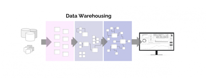
Understanding databases for storing, updating and analyzing data requires the understanding of the CAP Theorem. This is the second article of the article series Data Warehousing Basics.

Understanding NoSQL Databases by the CAP Theorem

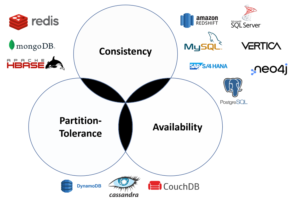
CAP theorem – or Brewer’s theorem – was introduced by the computer scientist Eric Brewer at Symposium on Principles of Distributed computing in 2000. The CAP stands for Consistency, Availability and Partition tolerance.

  • Consistency: Every read receives the most recent writes or an error. Once a client writes a value to any server and gets a response, it is expected to get afresh and valid value back from any server or node of the database cluster it reads from.
    Be aware that the definition of consistency for CAP means something different than to ACID (relational consistency).
  • Availability: The database is not allowed to be unavailable because it is busy with requests. Every request received by a non-failing node in the system must result in a response. Whether you want to read or write you will get some response back. If the server has not crashed, it is not allowed to ignore the client’s requests.
  • Partition tolerance: Databases which store big data will use a cluster of nodes that distribute the connections evenly over the whole cluster. If this system has partition tolerance, it will continue to operate despite a number of messages being delayed or even lost by the network between the cluster nodes.

CAP theorem applies the logic that  for a distributed system it is only possible to simultaneously provide  two out of the above three guarantees. Eric Brewer, the father of the CAP theorem, proved that we are limited to two of three characteristics, “by explicitly handling partitions, designers can optimize consistency and availability, thereby achieving some trade-off of all three.” (Brewer, E., 2012).

CAP Theorem Triangle

To recap, with the CAP theorem in relation to Big Data distributed solutions (such as NoSQL databases), it is important to reiterate the fact, that in such distributed systems it is not possible to guarantee all three characteristics (Availability, Consistency, and Partition Tolerance) at the same time.

Database systems designed to fulfill traditional ACID guarantees like relational database (management) systems (RDBMS) choose consistency over availability, whereas NoSQL databases are mostly systems designed referring to the BASE philosophy which prefer availability over consistency.

The CAP Theorem in the real world

Lets look at some examples to understand the CAP Theorem further and provewe cannot create database systems which are being consistent, partition tolerant as well as always available simultaniously.

AP – Availability + Partition Tolerance

If we have achieved Availability (our databases will always respond to our requests) as well as Partition Tolerance (all nodes of the database will work even if they cannot communicate), it will immediately mean that we cannot provide Consistency as all nodes will go out of sync as soon as we write new information to one of the nodes. The nodes will continue to accept the database transactions each separately, but they cannot transfer the transaction between each other keeping them in synchronization. We therefore cannot fully guarantee the system consistency. When the partition is resolved, the AP databases typically resync the nodes to repair all inconsistencies in the system.

A well-known real world example of an AP system is the Domain Name System (DNS). This central network component is responsible for resolving domain names into IP addresses and focuses on the two properties of availability and failure tolerance. Thanks to the large number of servers, the system is available almost without exception. If a single DNS server fails,another one takes over. According to the CAP theorem, DNS is not consistent: If a DNS entry is changed, e.g. when a new domain has been registered or deleted, it can take a few days before this change is passed on to the entire system hierarchy and can be seen by all clients.

CA – Consistency + Availability

Guarantee of full Consistency and Availability is practically impossible to achieve in a system which distributes data over several nodes. We can have databases over more than one node online and available, and we keep the data consistent between these nodes, but the nature of computer networks (LAN, WAN) is that the connection can get interrupted, meaning we cannot guarantee the Partition Tolerance and therefor not the reliability of having the whole database service online at all times.

Database management systems based on the relational database models (RDBMS) are a good example of CA systems. These database systems are primarily characterized by a high level of consistency and strive for the highest possible availability. In case of doubt, however, availability can decrease in favor of consistency. Reliability by distributing data over partitions in order to make data reachable in any case – even if computer or network failure – meanwhile plays a subordinate role.

CP – Consistency + Partition Tolerance

If the Consistency of data is given – which means that the data between two or more nodes always contain the up-to-date information – and Partition Tolerance is given as well – which means that we are avoiding any desynchronization of our data between all nodes, then we will lose Availability as soon as only one a partition occurs between any two nodes In most distributed systems, high availability is one of the most important properties, which is why CP systems tend to be a rarity in practice. These systems prove their worth particularly in the financial sector: banking applications that must reliably debit and transfer amounts of money on the account side are dependent on consistency and reliability by consistent redundancies to always be able to rule out incorrect postings – even in the event of disruptions in the data traffic. If consistency and reliability is not guaranteed, the system might be unavailable for the users.

CAP Theorem Venn Diagram

Conclusion

The CAP Theorem is still an important topic to understand for data engineers and data scientists, but many modern databases enable us to switch between the possibilities within the CAP Theorem. For example, the Cosmos DB von Microsoft Azure offers many granular options to switch between the consistency, availability and partition tolerance . A common misunderstanding of the CAP theorem that it´s none-absoluteness: “All three properties are more continuous than binary. Availability is continuous from 0 to 100 percent, there are many levels of consistency, and even partitions have nuances. Exploring these nuances requires pushing the traditional way of dealing with partitions, which is the fundamental challenge. Because partitions are rare, CAP should allow perfect C and A most of the time, but when partitions are present or perceived, a strategy is in order.” (Brewer, E., 2012).

How To Remotely Send R and Python Execution to SQL Server from Jupyter Notebooks

Introduction

Did you know that you can execute R and Python code remotely in SQL Server from Jupyter Notebooks or any IDE? Machine Learning Services in SQL Server eliminates the need to move data around. Instead of transferring large and sensitive data over the network or losing accuracy on ML training with sample csv files, you can have your R/Python code execute within your database. You can work in Jupyter Notebooks, RStudio, PyCharm, VSCode, Visual Studio, wherever you want, and then send function execution to SQL Server bringing intelligence to where your data lives.

This tutorial will show you an example of how you can send your python code from Juptyter notebooks to execute within SQL Server. The same principles apply to R and any other IDE as well. If you prefer to learn through videos, this tutorial is also published on YouTube here:


Environment Setup Prerequisites

  1. Install ML Services on SQL Server

In order for R or Python to execute within SQL, you first need the Machine Learning Services feature installed and configured. See this how-to guide.

  1. Install RevoscalePy via Microsoft’s Python Client

In order to send Python execution to SQL from Jupyter Notebooks, you need to use Microsoft’s RevoscalePy package. To get RevoscalePy, download and install Microsoft’s ML Services Python Client. Documentation Page or Direct Download Link (for Windows).

After downloading, open powershell as an administrator and navigate to the download folder. Start the installation with this command (feel free to customize the install folder): .\Install-PyForMLS.ps1 -InstallFolder “C:\Program Files\MicrosoftPythonClient”

Be patient while the installation can take a little while. Once installed navigate to the new path you installed in. Let’s make an empty folder and open Jupyter Notebooks: mkdir JupyterNotebooks; cd JupyterNotebooks; ..\Scripts\jupyter-notebook

Create a new notebook with the Python 3 interpreter:


To test if everything is setup, import revoscalepy in the first cell and execute. If there are no error messages you are ready to move forward.

Database Setup (Required for this tutorial only)

For the rest of the tutorial you can clone this Jupyter Notebook from Github if you don’t want to copy paste all of the code. This database setup is a one time step to ensure you have the same data as this tutorial. You don’t need to perform any of these setup steps to use your own data.

  1. Create a database

Modify the connection string for your server and use pyodbc to create a new database.

import pyodbc  
# creating a new db to load Iris sample in 
new_db_name = "MLRemoteExec" connection_string = "Driver=SQL Server;Server=localhost\MSSQLSERVER2017;Database={0};Trusted_Connection=Yes;" 

cnxn = pyodbc.connect(connection_string.format("master"), autocommit=True) 

cnxn.cursor().execute("IF EXISTS(SELECT * FROM sys.databases WHERE [name] = '{0}') DROP DATABASE {0}".format(new_db_name)) 

cnxn.cursor().execute("CREATE DATABASE " + new_db_name)

cnxn.close()

print("Database created") 
  1. Import Iris sample from SkLearn

Iris is a popular dataset for beginner data science tutorials. It is included by default in sklearn package.

from sklearn import datasetsimport pandas as pd
# SkLearn has the Iris sample dataset built in to the packageiris = datasets.load_iris()
df = pd.DataFrame(iris.data, columns=iris.feature_names)
  1. Use RecoscalePy APIs to create a table and load the Iris data

(You can also do this with pyodbc, sqlalchemy or other packages)

from revoscalepy import RxSqlServerData, rx_data_step
# Example of using RX APIs to load data into SQL table. You can also do this with pyodbc
table_ref = RxSqlServerData(connection_string=connection_string.format(new_db_name), table="Iris")rx_data_step(input_data = df, output_file = table_ref, overwrite = True)print("New Table Created: Iris")
print("Sklearn Iris sample loaded into Iris table")

Define a Function to Send to SQL Server

Write any python code you want to execute in SQL. In this example we are creating a scatter matrix on the iris dataset and only returning the bytestream of the .png back to Jupyter Notebooks to render on our client.

def send_this_func_to_sql():
    from revoscalepy import RxSqlServerData, rx_import
    from pandas.tools.plotting import scatter_matrix
    import matplotlib.pyplot as plt
    import io    
# remember the scope of the variables in this func are within our SQL Server Python Runtime
    connection_string = "Driver=SQL Server;Server=localhost\MSSQLSERVER2017; Database=MLRemoteExec;Trusted_Connection=Yes;"

# specify a query and load into pandas dataframe df
    sql_query = RxSqlServerData(connection_string=connection_string, sql_query = "select * from Iris")

    df = rx_import(sql_query)
    scatter_matrix(df)

# return bytestream of image created by scatter_matrix
    buf = io.BytesIO()
    plt.savefig(buf, format="png")
    buf.seek(0)
    return buf.getvalue()

Send execution to SQL

Now that we are finally set up, check out how easy sending remote execution really is! First, import revoscalepy. Create a sql_compute_context, and then send the execution of any function seamlessly to SQL Server with RxExec. No raw data had to be transferred from SQL to the Jupyter Notebook. All computation happened within the database and only the image file was returned to be displayed.

from IPython import display
import matplotlib.pyplot as plt 
from revoscalepy import RxInSqlServer, rx_exec# create a remote compute context with connection to SQL Server

sql_compute_context = RxInSqlServer(connection_string=connection_string.format(new_db_name))

# use rx_exec to send the function execution to SQL Server

image = rx_exec(send_this_func_to_sql, compute_context=sql_compute_context)[0]

# only an image was returned to my jupyter client. All data remained secure and was manipulated in my db.

display.Image(data=image)

While this example is trivial with the Iris dataset, imagine the additional scale, performance, and security capabilities that you now unlocked. You can use any of the latest open source R/Python packages to build Deep Learning and AI applications on large amounts of data in SQL Server. We also offer leading edge, high-performance algorithms in Microsoft’s RevoScaleR and RevoScalePy APIs. Using these with the latest innovations in the open source world allows you to bring unparalleled selection, performance, and scale to your applications.

Learn More

Check out SQL Machine Learning Services Documentation to learn how you can easily deploy your R/Python code with SQL stored procedures making them accessible in your ETL processes or to any application. Train and store machine learning models in your database bringing intelligence to where your data lives.

Other YouTube Tutorials:

Bringing intelligence to where data lives: Python & R embedded in T-SQL

Introduction

Did you know that you can write R and Python code within your T-SQL statements? Machine Learning Services in SQL Server eliminates the need for data movement. Instead of transferring large and sensitive data over the network or losing accuracy with sample csv files, you can have your R/Python code execute within your database. Easily deploy your R/Python code with SQL stored procedures making them accessible in your ETL processes or to any application. Train and store machine learning models in your database bringing intelligence to where your data lives.

You can install and run any of the latest open source R/Python packages to build Deep Learning and AI applications on large amounts of data in SQL Server. We also offer leading edge, high-performance algorithms in Microsoft’s RevoScaleR and RevoScalePy APIs. Using these with the latest innovations in the open source world allows you to bring unparalleled selection, performance, and scale to your applications.

If you are excited to try out SQL Server Machine Learning Services, check out the hands on tutorial below. If you do not have Machine Learning Services installed in SQL Server,you will first want to follow the getting started tutorial I published here: 

How-To Tutorial

In this tutorial, I will cover the basics of how to Execute R and Python in T-SQL statements. If you prefer learning through videos, I also published the tutorial on YouTube.

Basics

Open up SQL Server Management Studio and make a connection to your server. Open a new query and paste this basic example: (While I use Python in these samples, you can do everything with R as well)

EXEC sp_execute_external_script @language = N'Python',
@script = N'print(3+4)'

Sp_execute_external_script is a special system stored procedure that enables R and Python execution in SQL Server. There is a “language” parameter that allows us to choose between Python and R. There is a “script” parameter where we can paste R or Python code. If you do not see an output print 7, go back and review the setup steps in this article.

Parameter Introduction

Now that we discussed a basic example, let’s start adding more pieces:

EXEC sp_execute_external_script  @language =N'Python', 
@script = N' 
OutputDataSet = InputDataSet;
',
@input_data_1 =N'SELECT 1 AS Col1';

Machine Learning Services provides more natural communications between SQL and R/Python with an input data parameter that accepts any SQL query. The input parameter name is called “input_data_1”.
You can see in the python code that there are default variables defined to pass data between Python and SQL. The default variable names are “OutputDataSet” and “InputDataSet” You can change these default names like this example:

EXEC sp_execute_external_script  @language =N'Python', 
@script = N' 
MyOutput = MyInput;
',
@input_data_1_name = N'MyInput',
@input_data_1 =N'SELECT 1 AS foo',
@output_data_1_name =N'MyOutput';

As you executed these examples, you might have noticed that they each return a result with “(No column name)”? You can specify a name for the columns that are returned by adding the WITH RESULT SETS clause to the end of the statement which is a comma separated list of columns and their datatypes.

EXEC sp_execute_external_script  @language =N'Python', 
@script=N' 
MyOutput = MyInput;
',
@input_data_1_name = N'MyInput',
@input_data_1 =N'
SELECT 1 AS foo,
2 AS bar
',
@output_data_1_name =N'MyOutput'
WITH RESULT SETS ((MyColName int, MyColName2 int));

Input/Output Data Types

Alright, let’s discuss a little more about the input/output data types used between SQL and Python. Your input SQL SELECT statement passes a “Dataframe” to python relying on the Python Pandas package. Your output from Python back to SQL also needs to be in a Pandas Dataframe object. If you need to convert scalar values into a dataframe here is an example:

EXEC sp_execute_external_script  @language =N'Python', 
@script=N' 
import pandas as pd
c = 1/2
d = 1*2
s = pd.Series([c,d])
df = pd.DataFrame(s)
OutputDataSet = df
'

Variables c and d are both scalar values, which you can add to a pandas Series if you like, and then convert them to a pandas dataframe. This one shows a little bit more complicated example, go read up on the python pandas package documentation for more details and examples:

EXEC sp_execute_external_script  @language =N'Python', 
@script=N' 
import pandas as pd
s = {"col1": [1, 2], "col2": [3, 4]}
df = pd.DataFrame(s)
OutputDataSet = df
'

You now know the basics to execute Python in T-SQL!

Did you know you can also write your R and Python code in your favorite IDE like RStudio and Jupyter Notebooks and then remotely send the execution of that code to SQL Server? Check out these documentation links to learn more: https://aka.ms/R-RemoteSQLExecution https://aka.ms/PythonRemoteSQLExecution

Check out the SQL Server Machine Learning Services documentation page for more documentation, samples, and solutions. Check out these E2E tutorials on github as well.

Would love to hear from you! Leave a comment below to ask a question, or start a discussion!