Tag Archive for: Deep Learning

Spiky cubes, Pac-Man walking, empty M&M’s chocolate: curse of dimensionality

This is the first article of the article series Illustrative introductions on dimension reduction.

“Curse of dimensionality” means the difficulties of machine learning which arise when the dimension of data is higher. In short if the data have too many features like “weight,” “height,” “width,” “strength,” “temperature”…., that can undermine the performances of machine learning. The fact might be contrary to your image which you get from the terms “big” data or “deep” learning. You might assume that the more hints you have, the better the performances of machine learning are. There are some reasons for curse of dimensionality, and in this article I am going to introduce two major reasons below.

  1. High dimensional data usually have rich expressiveness, but usually training data are too poor for that.
  2. The behaviors of data points in high dimensional space are totally different from our common sense.

Through these topics, you will see that you always have to think about which features to use considering the number of data points.

*From now on I am going to talk about only Euclidean distance. If you are not sure what Euclidean distance means, please just keep it in mind that it is the type of distance most people wold have learnt in normal compulsory education.

1. Number of samples and degree of dimension

The most straightforward demerit of adding many features, or increasing dimensions of data, is the growth of computational costs. More importantly, however, you always have to think about the degree of dimensions in relation of the number of data points you have. Let me take a simple example in a book “Pattern Recognition and Machine Learning” by C. M. Bishop (PRML). This is an example of measurements of a pipeline. The figure below shows a comparison plot of 3 classes (red, green and blue), with parameter x_7 plotted against parameter x_6 out of 12 parameters.

* The meaning of data is not important in this article. If you are interested please refer to the appendix in PRML.

Assume that we are interested in classifying the cross in black into one of the three classes. One of the most naive ideas of this classification is dividing the graph into grids and labeling each grid depending on the number of samples in the classes (which are colored at the right side of the figure). And you can classify the test sample, the cross in black, into the class of the grid where the test sample is in. Thereby the cross is classified to the class in red.
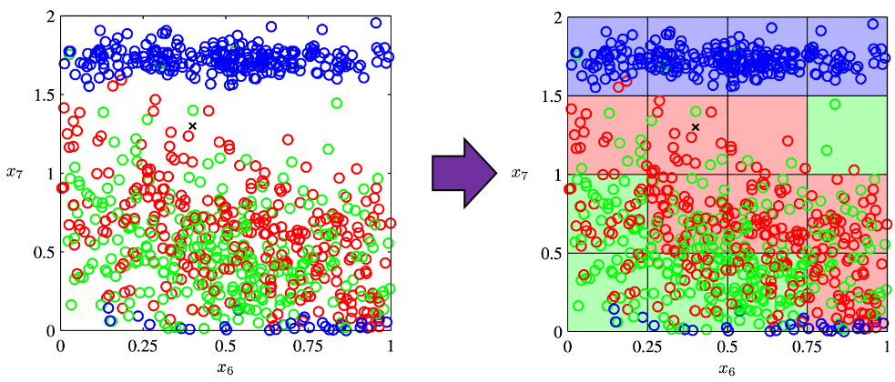
Source: C.M. Bishop, “Pattern Recognition and Machine Learning,” (2006), Springer, pp. 34-35

As I mentioned in the figure above, we used only two features out of 12 features in total. When the total number of data points is fixed and you add remaining ten axes/features one after another, what would happen? Let’s see what “adding axes/features” means. If you are talking about 1, 2, or 3 dimensional grids, you can visualize them. And as you can see from the figure below, if you make each 10^1, 10^2, 100^3 grids respectively in 1, 2, 3 dimensional spaces, the number of the small regions in the grids are respectively 10, 100, 1000. Even though you cannot visualize it anymore, you can make grids for more than 3 dimensional data. If you continue increasing the degree of dimension, the number of grids increases exponentially, and that can soon surpass the number of training data points. That means there would be a lot of empty spaces in such high dimensional grids. And the classifying method above: coloring each grid and classifying unknown samples depending on the colors of the grids, does not work out anymore because there would be a lot of empty grids.

* If you are still puzzled by the idea of “more than 3 dimensional grids,” you should not think too much about that now. It is enough if you can get some understandings on high dimensional data after reading the whole article of this.
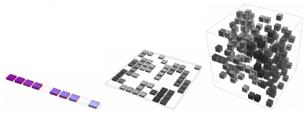
Source: Goodfellow and Yoshua Bengio and Aaron Courville, Deep Learning, (2016), MIT Press, p. 153

I said the method above is the most naive way, but other classical classification methods , for example k-nearest neighbors algorithm, are more or less base on a similar idea. Many of classical machine learning algorithms are based on the idea of smoothness prior, or local constancy prior. In short in classical ways, you  do not expect data to change so much in a small region, so you can expect unknown samples to be similar to data in vicinity. But that soon turns out to be problematic when the dimension of data is bigger because training data would be sparse because the area of multidimensional space grows exponentially as I mentioned above. And sometimes you would not be able to find training data around test data. Plus, in high dimensional data, you cannot treat distance in the same as you do in lower dimensional space. The ideas of “close,” “nearby,” or “vicinity” get more obscure in high dimensional data. That point is related to the next topic: the intuition have cultivated in normal life is not applicable to higher dimensional data.

2. Bizarre characteristics of high dimensional data

We form our sense of recognition in 3-dimensional ways in our normal life. Even though we can visualize only 1, 2, or 3 dimensional data, we can actually generalize the ideas in 1, 2, or 3 dimensional ideas to higher dimensions. For example 4 dimensional cubes, 100 dimensional spheres, or orthogonality in 255 dimensional space. Again, you cannot exactly visualize those ideas, and for many people, such high dimensional phenomenon are just imaginary matters on blackboards. Those high dimensional ideas are designed to retain some conditions just as well as 1, 2, or 3 dimensional space. Let’s take an example of spheres in several dimensional spaces. General spheres in any D-dimensional space can be defined as a set of any \boldsymbol{x}, such that |\boldsymbol{x} - \boldsymbol{c}| = r, where \boldsymbol{c} is the center point and r is length of radius. When \boldsymbol{x} is 2-dimensional, the spheres are called “circles.” When \boldsymbol{x} is 3-dimensional, the spheres are called “spheres” in our normal life, unless it is used in a conversation in a college cafeteria, by some students in mathematics department. And when \boldsymbol{x} is D-dimensional, they are called D-ball, and again, this is just a imaginary phenomenon on blackboard.

* Vectors and points are almost the same because all the vectors are denoted as “arrows” from the an origin point to sample data points.  The only difference is that when you use vectors, you have to consider their directions.

* “D-ball” is usually called “n-ball,” and in such context it is a sphere in a n-dimensional space. But please let me use the term “D-ball” in this article.
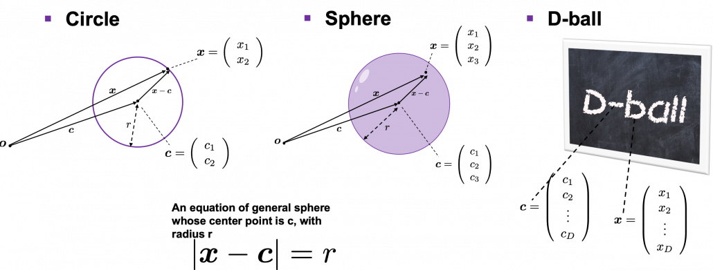
Not only spheres, but only many other ideas have been generalized to D-dimensional space, and many of them are indispensable also for data science. But there is one severe problem: the behaviors of data in high dimensional field is quite different from those in two or three dimensional space. To be concrete, in high dimensional field, cubes are spiky, you have to move like Pac-Man, and M & M’s Chocolate looks empty inside but tastes normal.

2.1: spiky cubes
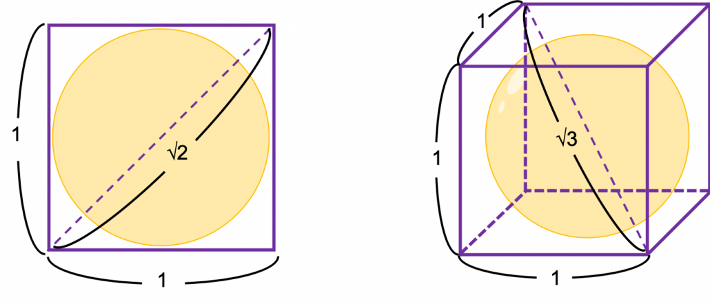
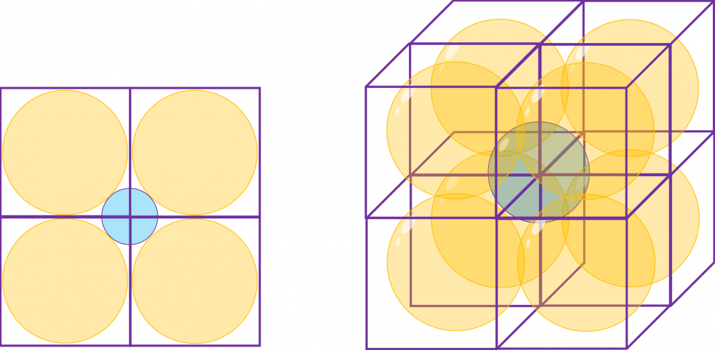
Let’s take a look at an elementary-school-level example of geometry first. Assume that you have several unit squares or unit cubes like below. In each of them a circle or sphere with diameter 1 is inscribed. The length of a diagonal line in each square is \sqrt{2}, and that in each cube is \sqrt{3}.

If you stack the squares or cubes as below, what are the length of diameters of the blue circle or sphere, circumscribing all the 4 orange circles or the 8 orange spheres?

The answers are, the diameter of the blue circle is \sqrt{2} - 1, and the diameter of the blue sphere is \sqrt{3} - 1.

Next let’s think about the same situation in higher dimensional space. Assume that there are some unit D-dimensional hypercubes stacked, in each of which a D-ball with diameter 1 is inscribed, touching all the surfaces inside. Then what is the length of the diameter of  a D-ball circumscribing all the unit D-ball in the hypercubes ? Given the results above, it ca be predicted that its diameter is \sqrt{D}  -1. If that is true, there is one strange point: \sqrt{D} - 1 can soon surpass 2: that means in the chart above the blue sphere will stick out of the stacked cubes. That sounds like a paradox, but with one hypothesis, the phenomenon makes sense: cubes become more spiky as the degree of dimension grows. This hypothesis is a natural deduction because diagonal lines of hyper cubes get longer, and the the center of each surface of hypercubes still touches the unit D-ball with diameter 1, inscribing inscribing inside each unit hypercube.
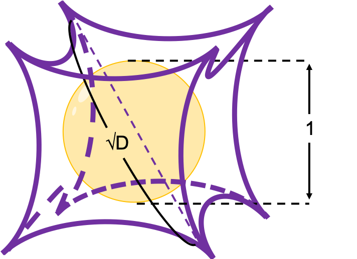
If you stack 4 hypercubes, the blue sphere circumscribing them will not stick out of the stacked hypercubes anymore like the figure below.

*Of course you cannot visualize what is going on in D-dimensional space, so the figure below is just a pseudo simulation of D-dimensional space in our 3-dimensional sense. I guess you have to stack more than four hyper cubes in higher dimensional data, but you cannot easily imagine what will go on in such space anymore.


*You can confirm the fact that hypercube gets more spiky as the degree of dimension growth, by comparing the volume of the hypercube and the volume of the D-ball inscribed inside the hypercube. Thereby you can prove that the volume of hypercube concentrates on the corners of the hypercube. Plus, as I mentioned the longest diagonal distance of hypercube gets longer as dimension degree increases. That is why hypercube is said to be spiky. For mathematical proof, please check the Exercise 1.19 of PRML.

2.2: Pac-Man walking

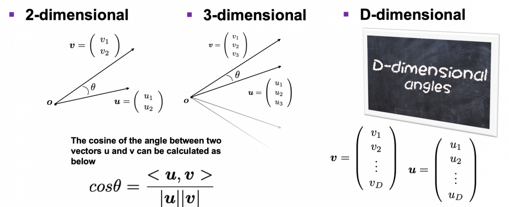
Next intriguing phenomenon in high dimensional field is that most of pairs of vectors in high dimensional space are orthogonal. In other words, if you select two random vectors in high dimensional space, the angle between them are mostly close to 90^\circ. Let’s see the general meaning of angle between two vectors in any dimensional spaces. Assume that the angle between two vectors \boldsymbol{u}, and \boldsymbol{v} is \theta, then cos\theta is calculated as cos\theta = \frac{<\boldsymbol{u}, \boldsymbol{v}>}{|\boldsymbol{u}||\boldsymbol{v}|}. In 1, 2, or 3 dimensional space, you can actually see the angle, but again you can define higher dimensional angle, which you cannot visualize anymore. And angles are sometimes used as similarity of two vectors.

* <\boldsymbol{u}, \boldsymbol{v}> is the inner product of \boldsymbol{u}, and \boldsymbol{v}.

Assume that you generate a pair of two points inside a D-dimensional unit sphere and make two vectors \boldsymbol{u}, and \boldsymbol{v} by connecting the origin point and those two points respectively. When D is 2, I mean spheres are circles in this case, any \theta are equally generated as in the chart below. The fact might be the same as your intuition.   How about in 3-dimensional space? In fact the distribution of \theta is not uniform. \theta = 90^\circ is the most likely to be generated. As I explain in the figure below, if you compare the area of cross section of a hemisphere and the area of a cone whose vertex is the center point of the sphere, you can see why.
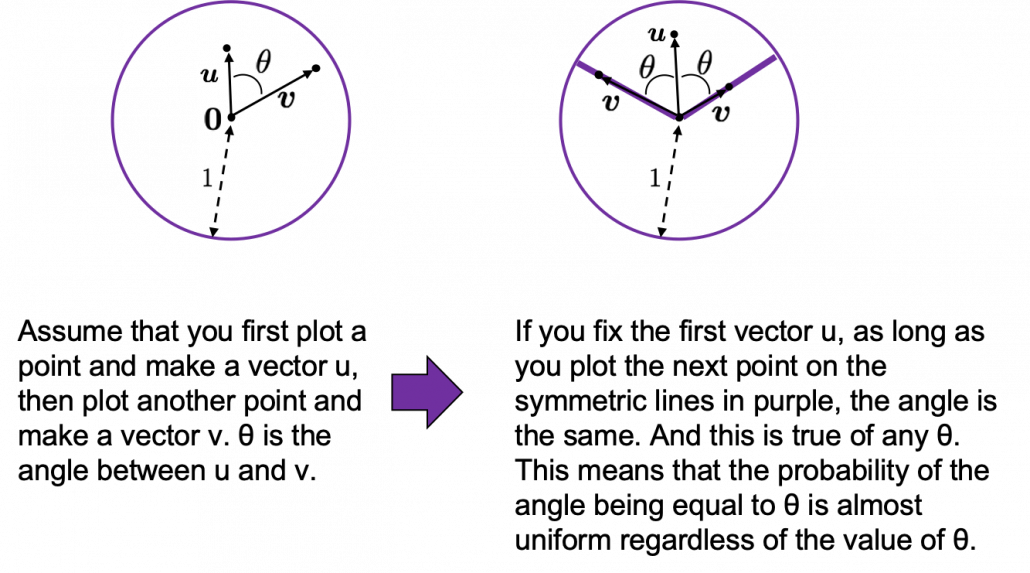
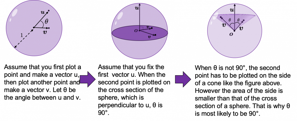
I generated 10000 random pairs of points in side a D-dimensional unit sphere, and calculated the angle between them. In other words I just randomly generated two D-dimensional vectors \boldsymbol{u} and \boldsymbol{v}, whose elements are randomly generated values between -1 and 1, and calculated the angle between them, repeating this process 10000 times. The chart below are the histograms of angle between pairs of generated vectors in respectively 2, 3, 50, and 100 dimensional space.

As I explained above, in 2-dimensional space, the distribution of \theta is almost uniform. However the distribution concentrates a little around 90^\circ in 3-dimensional space. You can see that the bigger the degree of dimension is, the more the angles of generated vectors concentrate around 90^\circ. That means most pairs of vectors in high dimensional space are close to orthogonal. Movements are also sequence of vectors, so when most pairs of movement vectors are orthogonal, that means you can only move like Pac-Man in such space.

Source: https://edition.cnn.com/style/article/pac-man-40-anniversary-history/index.html

* Of course I am talking about arcade Mac-Man game. Not Pac-Man in Super Smash Bros.  Retro RPG video games might have more similar playability, but in high dimensional space it is also difficult to turn back. At any rate, I think you have understood it is even difficult to move smoothly in high dimensional space, just like the first notorious Resident Evil on the first PS console also had terrible playability .

2.3: empty M & M’s chocolate

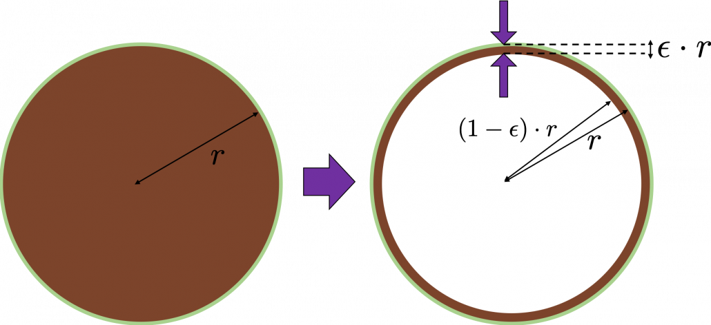
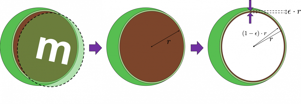
Let’s think about the proportion of the volume of the outermost \epsilon surface of general spheres with radius r. First, in 2 two dimensional space, spheres are circles. The area of the brown part of the circle below is \pi r^2. In order calculate the are of \epsilon \cdot r thick surface of the circle, you have only to subtract the area of \pi \{ (1 - \epsilon)\cdot r\} ^2. When \epsilon = 0.01, the area of outer most surface is \pi r^2 - \pi (0.99\cdot r)^2, and its proportion to the area of the whole circle is \frac{\pi r^2 - \pi (0.99\cdot r)^2}{\pi r^2} = 0.0199.

In case of 3-dimensional space, the value of a sphere with radius r is \frac{4}{3} \pi r^2, so the proportion of the \epsilon surface is calculated in the same way: \frac{\frac{4}{3} \pi r^3 -\frac{4}{3} \pi (0.99\cdot r)^2}{\frac{4}{3}\pi r^2} = 0.0297. Compared to the case in 2 dimensional space, the proportion is a little bigger.

How about in D-dimensional space? We have seen that even in  D-dimensional space the surface of a sphere, I mean D-ball, can be defined as a set of any points whose distance from the center point is all r. And it is known that the volume of D-ball is defined as below.

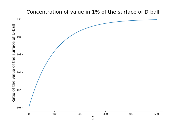
\Gamma () is called gamma function, but in this article it is not so important. The most important point now is, if you discuss any D-ball, their volume only depends on their radius r. That meas the proportion of outer \epsilon surface of D-ball is calculated as \frac{\pi r^2 - \pi \{ (1 - \epsilon)\cdot r\} ^2}{\pi r^2}. When \epsilon is 0.01, the proportion of the 1% surface of D-ball changes like in the chart below.

* And of course when D is 2,  \frac{\pi ^{(\frac{D}{2})}}{\Gamma (\frac{D}{2} + 1)} = \pi, and when D is 3 ,  \frac{\pi ^{(\frac{D}{2})}}{\Gamma (\frac{D}{2} + 1)} = \frac{4}{3} \pi

You can see that when D is over 400, around 90% of volume is concentrated in the very thin 1% surface of D-ball. That is why, in high dimensional space, M & M’s chocolate look empty but tastes normal: all the chocolate are concentrated beneath the sugar coating.

More interestingly, even if you choose any points as a central point of a sphere with radius r, the other points are squashed to the surface of the sphere, even if all the data points are uniformly distributed. This situation is problematic for classical machine learning algorithms, which are often based on the Euclidean distances between pairs of two sample data points: if you go from the central point to another sample point, the possibility of finding the point within (1 - \epsilon)\cdot r radius of the center is almost zero. But if you reach the outermost \epsilon part of the surface of the sphere, most data points are there. However, for one of the data points in the surface, any other data points are distant in the same way.

Inside M & M’s chocolate is a mysterious world.

Source: https://hipwallpaper.com/mms-wallpapers/

You have seen that using high dimensional data can be problematic in many ways. Data science and machine learning are largely based on one idea: you can find a lower dimensional meaningful and easier structure in data. In the next articles I am going to introduce some famous dimension reduction algorithms. And hopefully I would like to give some deeper insights in to these algorithms, in straightforward ways.

* I could not explain the relationships of variance and bias of data. This is also a very important factor when you think about dimensionality of data. I hope I can write about this topic someday. You can also look it up if you are interested.

* I make study materials on machine learning, sponsored by DATANOMIQ. I do my best to make my content as straightforward but as precise as possible. I include all of my reference sources. If you notice any mistakes in my materials, including grammatical errors, please let me know (email: yasuto.tamura@datanomiq.de). And if you have any advice for making my materials more understandable to learners, I would appreciate hearing it.

Simple RNN

LSTM back propagation: following the flows of variables

First of all, the summary of this article is: please just download my Power Point slides which I made and be patient, following the equations.

I am not supposed to use so many mathematics when I write articles on Data Science Blog. However using little mathematics when I talk about LSTM backprop is like writing German, never caring about “der,” “die,” “das,” or speaking little English in English classes (which most high school English teachers in Japan do) or writing Japanese without using any Chinese characters (which looks like a terrible handwriting by a drug addict). In short, that is ridiculous. And all the precise equations of LSTM backprop, written on a Blog is not a comfortable thing to see. So basically the whole of this article is an advertisement on my PowerPoint slides, sponsored by DATANOMIQ, and I can just give you some tips to get ready for the most tiresome part of understanding LSTM here.

*This article is the fifth article of “A gentle introduction to the tiresome part of understanding RNN.”

 *In this article “Densely Connected Layers” is written as “DCL,” and “Convolutional Neural Network” as “CNN.”

1. Chain rules

This article is virtually an article on chain rules of differentiation. Even if you have clear understandings on chain rules, I recommend you to take a look at this section. If you have written down all the equations of back propagation of DCL, you would have seen what chain rules are. Even simple chain rules for backprop of normal DCL can be difficult to some people, but when it comes to backprop of LSTM, it is a pure torture.  I think using graphical models would help you understand what chain rules are like. Graphical models are basically used to describe the relations of variables and functions in probabilistic models, so to be exact I am going to use “something like graphical models” in this article. Not that this is a common way to explain chain rules.

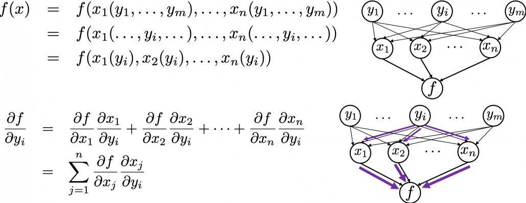
First, let’s think about the simplest type of chain rule. Assume that you have a function f=f(x)=f(x(y)), and relations of the functions are displayed as the graphical model at the left side of the figure below. Variables are a type of function, so you should think that every node in graphical models denotes a function. Arrows in purple in the right side of the chart show how information propagate in differentiation.

Next, if you a function f , which has two variances  x_1 and x_2. And both of the variances also share two variances  y_1 and y_2. When you take partial differentiation of f with respect to y_1 or y_2, the formula is a little tricky. Let’s think about how to calculate \frac{\partial f}{\partial y_1}. The variance y_1 propagates to f via x_1 and x_2. In this case the partial differentiation has two terms as below.

In chain rules, you have to think about all the routes where a variance can propagate through. If you generalize chain rules, that is like below, and you need to understand chain rules in this way to understanding any types of back propagation.

The figure above shows that if you calculate partial differentiation of f with respect to y_i, the partial differentiation has n terms in total because y_i propagates to f via n variances. In order to understand backprop of LSTM, you constantly have to care about the flow of variances, which I showed as arrows in purple above.

2. Chain rules in LSTM

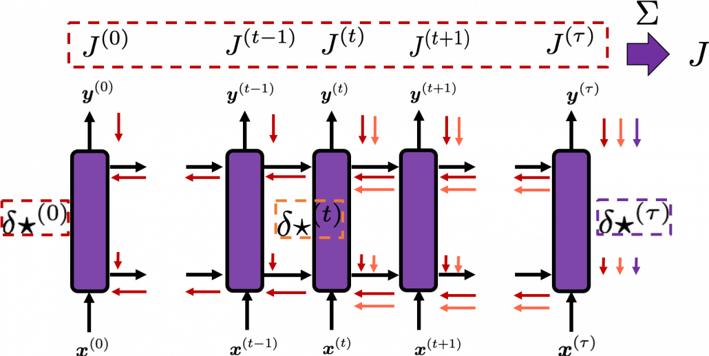
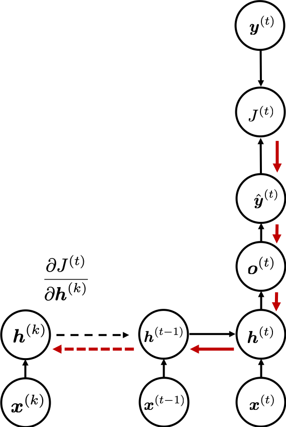
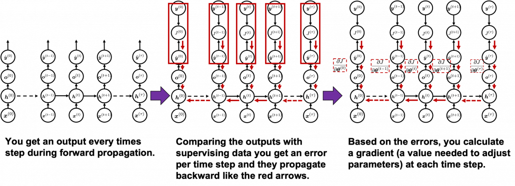
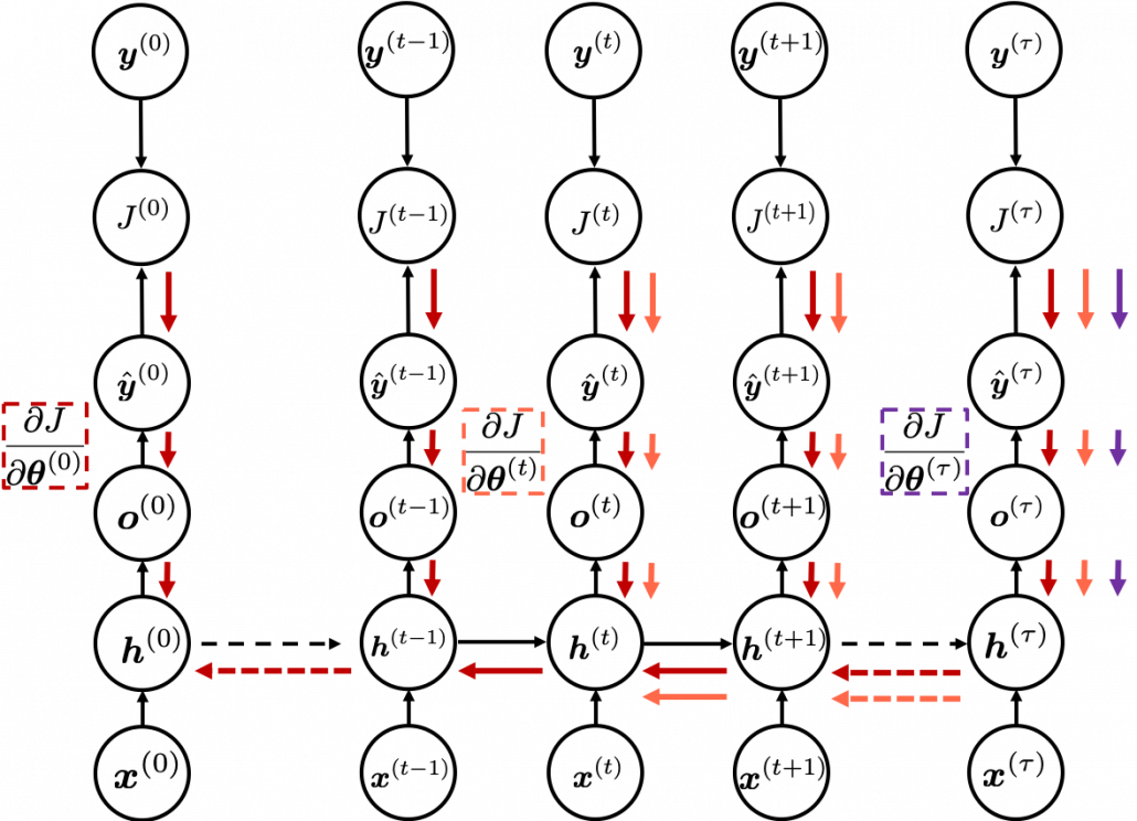
I would like you to remember the figure below, which I used in the second article to show how errors propagate backward during backprop of simple RNNs. After forward propagation, first of all, you need to calculate \frac{\partial J}{\partial \boldsymbol{\theta}^{(t)}}, gradients of the error function with respect to parameters, at every time step. But you have to be careful that even though these gradients depend on time steps, the parameters \boldsymbol{\theta} do not depend on time steps.

*As I mentioned in the second article I personally think \frac{\partial J}{\partial \boldsymbol{\theta}^{(t)}} should be rather denoted as (\frac{\partial J}{\partial \boldsymbol{\theta}})^{(t)} because parameters themselves do not depend on time. The textbook by MIT press also partly use the former notation. And you are likely to encounter this type of notation, so I think it is not bad to get ready for both.

The errors at time step (t) propagate backward to all the \boldsymbol{h} ^{(s)}, (s \leq t). Conversely, in order to calculate \frac{\partial J}{\partial \boldsymbol{\theta}^{(t)}} errors flowing from J^{(s)},  (s \geq t). In the chart you need arrows of errors in purple for the gradient in a purple frame, orange arrows for gradients in orange frame, red arrows for gradients in red frame. And you need to sum up \frac{\partial J}{\partial \boldsymbol{\theta}^{(t)}} to calculate \frac{\partial J}{\partial \boldsymbol{\theta}} = \sum_{t}{\frac{\partial J}{\partial \boldsymbol{\theta}^{(t)}}}, and you need this gradient \frac{\partial J}{\partial \boldsymbol{\theta}} to renew parameters, one time.

At an RNN block level, the flows of errors and how to renew parameters are the same in LSTM backprop, but the flow of errors inside each block is much more complicated in LSTM backprop. And in this article and my PowerPoint slides, I use a special notation to denote errors: \delta \star  ^{(t)}= \frac{\partial J^{(t)}}{\partial \star}

* Again, please be careful of what \delta \star  ^{(t)} means. Neurons depend on time steps, but parameters do not depend on time steps. So if \star are neurons,  \delta \star  ^{(t)}= \frac{\partial J}{ \partial \star ^{(t)}}, but when \star are parameters, \delta \star  ^{(t)}= \frac{\partial J^{(t)}}{ \partial \star} should be rather denoted like \delta \star  ^{(t)}= (\frac{\partial J}{ \partial \star ^{(t)}}). In the Space Odyssey paper\boldsymbol{\star} are not used as parameters, but in my PowerPoint slides and some other materials, \boldsymbol{\star} are used also as parameteres.

As I wrote in the last article, you calculate \boldsymbol{f}^{(t)}, \boldsymbol{i}^{(t)}, \boldsymbol{z}^{(t)}, \boldsymbol{o}^{(t)} as below. Unlike the last article, I also added the terms of peephole connections in the equations below, and I also added the variances \bar{\boldsymbol{f}^{(t)}}, \bar{\boldsymbol{i}^{(t)}}, \bar{\boldsymbol{z}^{(t)}}, \bar{\boldsymbol{o}^{(t)}} for convenience.

  • \boldsymbol{\bar{f}}^{(t)}=\boldsymbol{W}_{for} \cdot \boldsymbol{x}^{(t)} + \boldsymbol{R}_{for} \cdot \boldsymbol{y}^{(t-1)} + \boldsymbol{p}_{for}\odot \boldsymbol{c}^{(t-1)} + \boldsymbol{b}_{for}
  • \boldsymbol{\bar{i}}^{(t)}=\boldsymbol{W}_{in} \cdot \boldsymbol{x}^{(t)} + \boldsymbol{R}_{in} \cdot \boldsymbol{y}^{(t-1)} + \boldsymbol{p}_{in}\odot \boldsymbol{c}^{(t-1)} + \boldsymbol{b}_{in}
  • \boldsymbol{\bar{z}}^{(t)}=\boldsymbol{W}_z \cdot \boldsymbol{x}^{(t)} + \boldsymbol{R}_z \cdot \boldsymbol{y}^{(t-1)} + \boldsymbol{b}_z
  • \boldsymbol{\bar{o}}^{(t)}=\boldsymbol{W}_{out} \cdot \boldsymbol{x}^{(t)} + \boldsymbol{R}_{out} \cdot \boldsymbol{y}^{(t-1)} + \boldsymbol{p}_{out}\odot \boldsymbol{c}^{(t)} + \boldsymbol{b}_{out}
  • \boldsymbol{f}^{(t)}=\sigma( \boldsymbol{\bar{f}}^{(t)})
  • \boldsymbol{i}^{(t)}=\sigma(\boldsymbol{\bar{i}}^{(t)})
  • \boldsymbol{z}^{(t)}=tanh(\boldsymbol{\bar{z}}^{(t)})
  • \boldsymbol{o}^{(t)}=\sigma(\boldsymbol{\bar{o}}^{(t)})

With  Hadamar product operator, the renewed cell and the output are calculated as below.

  • \boldsymbol{c}^{(t)} = \boldsymbol{z}^{(t)}\odot \boldsymbol{i}^{(t)} + \boldsymbol{c}^{(t-1)} \odot \boldsymbol{f}^{(t)}
  • \boldsymbol{y}^{(t)} = \boldsymbol{o}^{(t)} \odot tanh(\boldsymbol{c}^{(t)})

In this article I would rather give instructions on how to read my PowerPoint slide. Just as general backprop, you need to calculate gradients of error functions with respect to parameters, such as \delta \boldsymbol{W}_{\star}, \delta \boldsymbol{R}_{\star}, \delta \boldsymbol{p}_{\star}, \delta \boldsymbol{b}_{\star}, where \star is either of \{z, in, for, out \}. And just as backprop of simple RNNs, in order to calculate gradients with respect to parameters, you need to calculate errors of neurons, that is gradients of error functions with respect to neurons, such as \delta \boldsymbol{f}^{(t)}, \delta \boldsymbol{i}^{(t)}, \delta \boldsymbol{z}^{(t)}, \delta \boldsymbol{o}^{(t)}.

*Again and again, keep it in mind that neurons depend on time steps, but parameters do not depend on time steps.

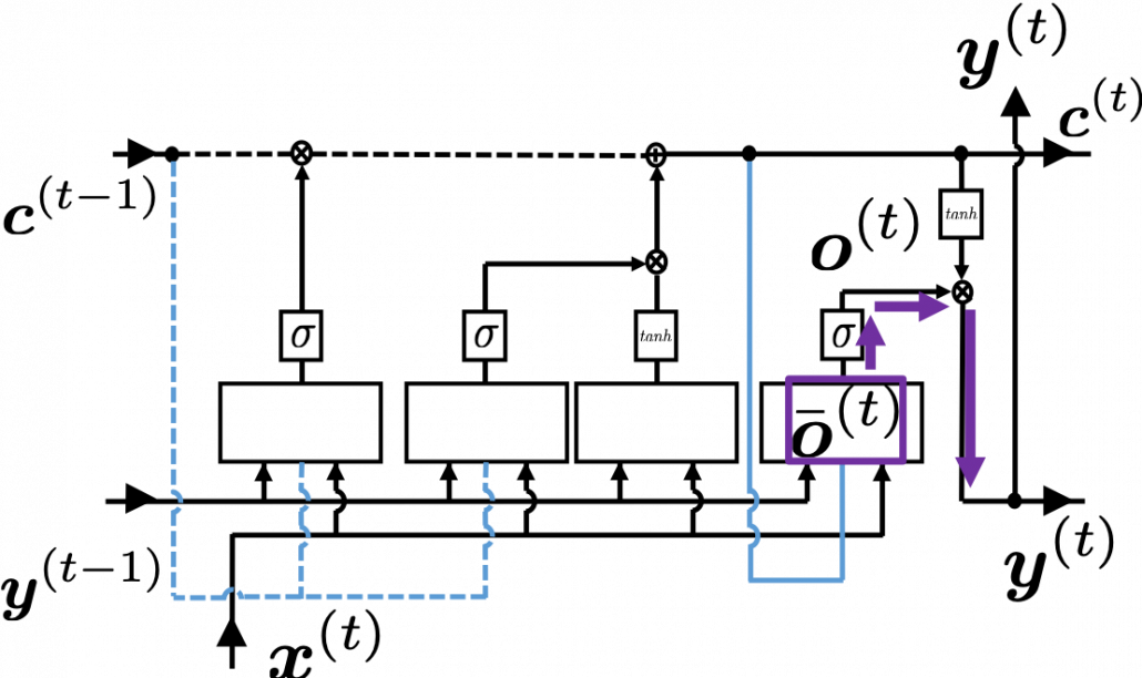
When you calculate gradients with respect to neurons, you can first calculate \delta \boldsymbol{y}^{(t)}, but the equation for this error is the most difficult, so I recommend you to put it aside for now. After calculating \delta \boldsymbol{y}^{(t)}, you can next calculate \delta \bar{\boldsymbol{o}}^{(t)}= \frac{\partial J^{(t)}}{ \partial \bar{\boldsymbol{o}}^{(t)}}. If you see the LSTM block below as a graphical model which I introduced, the information of \bar{\boldsymbol{o}}^{(t)} flow like the purple arrows. That means, \bar{\boldsymbol{o}}^{(t)} affects J only via \boldsymbol{y}^{(t)}, and this structure is equal to the first graphical model which I have introduced above. And if you calculate \bar{\boldsymbol{o}}^{(t)} element-wise, you get the equation \delta \bar{o}_{k}^{(t)}=\frac{\partial J}{\partial \bar{o}_{k}^{(t)}}= \frac{\partial J}{\partial y_{k}^{(t)}} \frac{\partial y_{k}^{(t)}}{\partial \bar{o}_{k}^{(t)}}.

*The k is an index of an element of vectors. If you can calculate element-wise gradients, it is easy to understand that as differentiation of vectors and matrices.

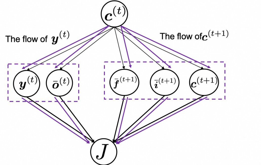
Next you can calculate \delta \boldsymbol{c}^{(t)}, and chain rules are very important in this process. The flow of \delta \boldsymbol{c}^{(t)} to J can be roughly divided into two streams: the one flows to J as \bodlsymbol{y}^{(t)}, and the one flows to J as \bodlsymbol{c}^{(t+1)}. And the stream from \bodlsymbol{c}^{(t)} to \bodlsymbol{y}^{(t)} also have two branches: the one via \bar{\boldsymbol{o}}^{(t)} and the one which directly converges as  \bodlsymbol{y}^{(t)}. Just as well, the stream from \bodlsymbol{c}^{(t)} to \bodlsymbol{c}^{(t+1)} also have three branches: the ones via \bar{\boldsymbol{f}}^{(t)}, \bar{\boldsymbol{i}}^{(t)}, and the one which directly converges as \bodlsymbol{c}^{(t+1)}.

If you see see these flows as graphical a graphical model, that would be like the figure below.

According to this graphical model, you can calculate \delta \boldsymbol{c} ^{(t)} element-wise as below.

* TO BE VERY HONEST I still do not fully understand why we can apply chain rules like above to calculate \delta \boldsymbol{c}^{(t)}. When you apply the formula of chain rules, which I showed in the first section, to this case, you have to be careful of where to apply partial differential operators \frac{\partial}{ \partial c_{k}^{(t)}}. In the case above, in the part \frac{\partial y_{k}^{(t)}}{\partial c_{k}^{(t)}} the partial differential operator only affects tanh(c_{k}^{(t)}) of o_{k}^{(t)} \cdot tanh(c_{k}^{(t)}), and in the part \frac{\partial c_{k}^{(t+1)}}{\partial c_{k}^{(t)}}, the partial differential operator \frac{\partial}{\partial c_{k}^{(t)}} only affects the part c_{k}^{(t)} of the term c^{t}_{k} \cdot f_{k}^{(t+1)}. In the \frac{\partial \bar{o}_{k}^{(t)}}{\partial c_{k}^{(t)}} part, only (p_{out})_{k} \cdot c_{k}^{(t)},  in the \frac{\partial \bar{i}_{k}^{(t+1)}}{\partial c_{k}^{(t)}} part, only (p_{in})_{k} \cdot c_{k}^{(t)}, and in the \frac{\partial \bar{f}_{k}^{(t+1)}}{\partial c_{k}^{(t)}} part, only (p_{in})_{k} \cdot c_{k}^{(t)}. But some other parts, which are not affected by \frac{\partial}{ \partial c_{k}^{(t)}} are also functions of c_{k}^{(t)}. For example o_{k}^{(t)} of o_{k}^{(t)} \cdot tanh(c_{k}^{(t)}) is also a function of c_{k}^{(t)}. And I am still not sure about the logic behind where to affect those partial differential operators.

*But at least, these are the only decent equations for LSTM backprop which I could find, and a frequently cited paper on LSTM uses implementation based on these equations. Computer science is more of practical skills, rather than rigid mathematical logic. It  If you have any comments or advice on this point, please let me know.

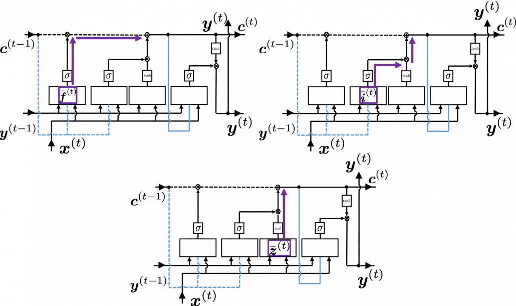
Calculating \delta \bar{\boldsymbol{f}}^{(t)}, \delta \bar{\boldsymbol{i}}^{(t)}, \delta \bar{\boldsymbol{z}}^{(t)} are also relatively straigtforward as calculating \delta \bar{\boldsymbol{o}}^{(t)}. They all use the first type of chain rule in the first section. Thereby you can get these gradients: \delta \bar{f}_{k}^{(t)}=\frac{\partial J}{ \partial \bar{f}_{k}^{(t)}} =\frac{\partial J}{\partial c_{k}^{(t)}} \frac{\partial c_{k}^{(t)}}{ \partial \bar{f}_{k}^{(t)}}, \delta \bar{i}_{k}^{(t)}=\frac{\partial J}{\partial \bar{i}_{k}^{(t)}} =\frac{\partial J}{\partial c_{k}^{(t)}} \frac{\partial c_{k}^{(t)}}{ \partial \bar{i}_{k}^{(t)}}, and \delta \bar{z}_{k}^{(t)}=\frac{\partial J}{\partial \bar{z}_{k}^{(t)}} =\frac{\partial J}{\partial c_{k}^{(t)}} \frac{\partial c_{k}^{(t)}}{ \partial \bar{i}_{k}^{(t)}}.

All the gradients which we have calculated use the error \delta \boldsymbol{y}^{(t)}, but when it comes to calculating \delta \boldsymbol{y}^{(t)}….. I can only say “Please be patient. I did my best in my PowerPoint slides to explain that.” It is not a kind of process which I want to explain on Word Press. In conclusion you get an error like this: \delta \boldsymbol{y}^{(t)}=\frac{\partial J^{(t)}}{\partial \boldsymbol{y}^{(t)}} + \boldsymbol{R}_{for}^{T} \delta \bar{\boldsymbol{f}}^{(t+1)} + \boldsymbol{R}_{in}^{T}\delta \bar{\boldsymbol{i}}^{(t+1)} + \boldsymbol{R}_{out}^{T}\delta \bar{\boldsymbol{o}}^{(t+1)} + \boldsymbol{R}_{z}^{T}\delta \bar{\boldsymbol{z}}^{(t+1)}, and the flows of \boldsymbol{y}^{(t)} are as blow.

Combining the gradients we have got so far, we can calculate gradients with respect to parameters. For concrete results, please check the Space Odyssey paper or my PowerPoint slide.

3. How LSTMs tackle exploding/vanishing gradients problems

*If you are allergic to mathematics, you should not read this section or download my PowerPoint slide.

*Part of this section is more or less subjective, so if you really want to know how LSTM mitigate the problems, I highly recommend you to also refer to other materials. But at least I did my best for this article.

LSTMs do not completely solve, vanishing gradient problems. They mitigate vanishing/exploding gradient problems. I am going to roughly explain why they can tackle those problems. I think you find many explanations on that topic, but many of them seems to have some mathematical mistakes (even the slide used in a lecture in Stanford University) and I could not partly agree with some statements. I also could not find any papers or materials which show the whole picture of how LSTMs can tackle those problems. So in this article I am only going to give instructions on the most mainstream way to explain this topic.

First let’s see how gradients actually “vanish” or “explode” in simple RNNs. As I in the second article of this series, simple RNNs propagate forward as the equations below.

  • \boldsymbol{a}^{(t)} = \boldsymbol{b} + \boldsymbol{W} \cdot \boldsymbol{h}^{(t-1)} + \boldsymbol{U} \cdot \boldsymbol{x}^{(t)}
  • \boldsymbol{h}^{(t)}= g(\boldsymbol{a}^{(t)})
  • \boldsymbol{o}^{(t)} = \boldsymbol{c} + \boldsymbol{V} \cdot \boldsymbol{h}^{(t)}
  • \hat{\boldsymbol{y}} ^{(t)} = f(\boldsymbol{o}^{(t)})

And every time step, you get an error function J^{(t)}. Let’s consider the gradient of J^{(t)} with respect to \boldsymbol{h}^{(k)}, that is the error flowing from J^{(t)} to \boldsymbol{h}^{(k)}. This error is the most used to calculate gradients of the parameters.

If you calculate this error more concretely, \frac{\partial J^{(t)}}{\partial \boldsymbol{h}^{(k)}} = \frac{\partial J^{(t)}}{\partial \boldsymbol{h}^{(t)}} \frac{\partial \boldsymbol{h}^{(t)}}{\partial \boldsymbol{h}^{(t-1)}} \cdots \frac{\partial \boldsymbol{h}^{(k+2)}}{\partial \boldsymbol{h}^{(k+1)}} \frac{\partial \boldsymbol{h}^{(k+1)}}{\partial \boldsymbol{h}^{(k)}} = \frac{\partial J^{(t)}}{\partial \boldsymbol{h}^{(t)}} \prod_{k< s \leq t} \frac{\partial \boldsymbol{h}^{(s)}}{\partial \boldsymbol{h}^{(s-1)}}, where \frac{\partial \boldsymbol{h}^{(s)}}{\partial \boldsymbol{h}^{(s-1)}} = \boldsymbol{W} ^T \cdot diag(g'(\boldsymbol{b} + \boldsymbol{W}\cdot \boldsymbol{h}^{(s-1)} + \boldsymbol{U}\cdot \boldsymbol{x}^{(s)})) = \boldsymbol{W} ^T \cdot diag(g'(\boldsymbol{a}^{(s)})).

* If you see the figure as a type of graphical model, you should be able to understand the why chain rules can be applied as the equation above.

*According to this paper \frac{\partial \boldsymbol{h}^{(s)}}{\partial \boldsymbol{h}^{(s-1)}}  = \boldsymbol{W} ^T \cdot diag(g'(\boldsymbol{a}^{(s)})), but it seems that many study materials and web sites are mistaken in this point.

Hence \frac{\partial J^{(t)}}{\partial \boldsymbol{h}^{(k)}} = \frac{\partial J^{(t)}}{\partial \boldsymbol{h}^{(t)}} \prod_{k< s \leq t} \boldsymbol{W} ^T \cdot diag(g'(\boldsymbol{a}^{(s)})) = \frac{\partial J^{(t)}}{\partial \boldsymbol{h}^{(t)}} (\boldsymbol{W} ^T )^{(t - k)} \prod_{k< s \leq t} diag(g'(\boldsymbol{a}^{(s)})). If you take norms of the members you get an equality \left\lVert \frac{\partial J^{(t)}}{\partial \boldsymbol{h}^{(k)}} \right\rVert \leq \left\lVert \frac{\partial J^{(t)}}{\partial \boldsymbol{h}^{(t)}} \right\rVert \left\lVert \boldsymbol{W} ^T \right\rVert ^{(t - k)} \prod_{k< s \leq t} \left\lVert diag(g'(\boldsymbol{a}^{(s)}))\right\rVert. I will not go into detail anymore, but it is known that according to this inequality, multiplication of weight vectors exponentially converge to 0 or to infinite number.

We have seen that the error \frac{\partial J^{(t)}}{\partial \boldsymbol{h}^{(k)}} is the main factor causing vanishing/exploding gradient problems. In case of LSTM, \frac{\partial J^{(t)}}{\partial \boldsymbol{c}^{(k)}} is an equivalent. For simplicity, let’s calculate only \frac{\partial \boldsymbol{c}^{(t)}}{\partial \boldsymbol{c}^{(t-1)}}, which is equivalent to \frac{\partial \boldsymbol{h}^{(t)}}{\partial \boldsymbol{h}^{(t-1)}} of simple RNN backprop.

* Just as I noted above, you have to be careful of which part the partial differential operator \frac{\partial}{\partial \boldsymbol{c}^{(t-1)}} affects in the chain rule above. That is, you need to calculate \frac{\partial}{\partial \boldsymbol{c}^{(t-1)}} (\boldsymbol{c}^{(t-1)} \odot \boldsymbol{f}^{(t)}), and the partial differential operator only affects \boldsymbol{c}^{(t-1)}. I think this is not a correct mathematical notation, but please forgive me for doing this for convenience.

If you continue calculating the equation above more concretely, you get the equation below.

I cannot mathematically explain why, but it is known that this characteristic of gradients of LSTM backprop mitigate the vanishing/exploding gradient problem. We have seen that if you take a norm of \frac{\partial J^{(t)}}{\partial \boldsymbol{h}^{(k)}}, that is equal or smaller than repeated multiplication of the norm of the same weight matrix, and that soon leads to vanishing/exploding gradient problem. But according to the equation above, even if you take a norm of repeatedly multiplied \frac{\partial \boldsymbol{c}^{(t)}}{\partial \boldsymbol{c}^{(t-1)}}, its norm cannot be evaluated with a simple value like repeated multiplication of the norm of the same weight matrix. The outputs of each gate are different from time steps to time steps, and that adjust the value of \frac{\partial \boldsymbol{c}^{(t)}}{\partial \boldsymbol{c}^{(t-1)}}.

*I personally guess the item diag(\boldsymbol{f}^{(t)}) is every effective. The unaffected value of can directly diag(\boldsymbol{f}^{(t)}) adjust the value of \frac{\partial \boldsymbol{c}^{(t)}}{\partial \boldsymbol{c}^{(t-1)}}. And as a matter of fact, it is known that performances of LSTM drop the most when you gite rid of forget gates.

When it comes to tackling exploding gradient problems, there is a much easier technique called gradient clipping. This algorithm is very simple: you just have to adjust the size of gradient so that the absolute value of gradient is under a threshold at every time step. Imagine that you decide in which direction to move by calculating gradients, but when the footstep is going to be too big, you just adjust the size of footstep to the threshold size you have set. In a pseudo code, write a gradient clipping part only with two line code as below.

*\boldsymbol{g} is a gradient at the time step threshold is the maximum size of the “step.”

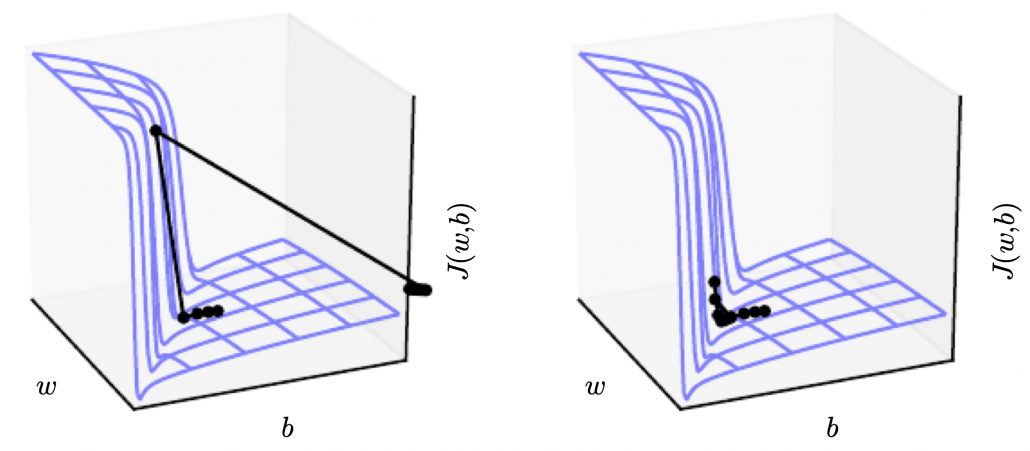
The figure below, cited from a deep learning text from MIT press textbook, is a good and straightforward explanation on gradient clipping.It is known that a strongly nonlinear function, such as error functions of RNN, can have very steep or plain areas. If you artificially visualize the idea in 3-dimensional space, as the surface of a loss function J with two variants w, b, that means the loss function J has plain areas and very steep cliffs like in the figure.Without gradient clipping, at the left side, you can see that the black dot all of a sudden climb the cliff and could jump to an unexpected area. But with gradient clipping, you avoid such “big jumps” on error functions.

Source: Source: Goodfellow and Yoshua Bengio and Aaron Courville, Deep Learning, (2016), MIT Press, 409p


I am glad that I have finally finished this article series. I am not sure how many of the readers would have read through all of the articles in this series, including my PowerPoint slides. I bet that is not so many. I spent a great deal of my time for making these contents, but sadly even when I was studying LSTM, it was becoming old-fashioned, at least in natural language processing (NLP) field: a very promising algorithm named Transformer has been replacing the position of LSTM. Deep learning is a very fast changing field. I also would like to make illustrative introductions on attention mechanism in NLP, from seq2seq model to Transformer. And I think LSTM would still remain as one of the algorithms in sequence data processing, such as hidden Hidden Markov model, or particle filter.

Simple RNN

Understanding LSTM forward propagation in two ways

*This article is only for the sake of understanding the equations in the second page of the paper named “LSTM: A Search Space Odyssey”. If you have no trouble understanding the equations of LSTM forward propagation, I recommend you to skip this article and go the the next article.

1. Preface

I  heard that in Western culture, smart people write textbooks so that other normal people can understand difficult stuff, and that is why textbooks in Western countries tend to be bulky, but also they are not so difficult as they look. On the other hand in Asian culture, smart people write puzzling texts on esoteric topics, and normal people have to struggle to understand what noble people wanted to say. Publishers also require the authors to keep the texts as short as possible, so even though the textbooks are thin, usually students have to repeat reading the textbooks several times because usually they are too abstract.

Both styles have cons and pros, and usually I prefer Japanese textbooks because they are concise, and sometimes it is annoying to read Western style long texts with concrete straightforward examples to reach one conclusion. But a problem is that when it comes to explaining LSTM, almost all the text books are like Asian style ones. Every study material seems to skip the proper steps necessary for “normal people” to understand its algorithms. But after actually making concrete slides on mathematics on LSTM, I understood why: if you write down all the equations on LSTM forward/back propagation, that is going to be massive, and actually I had to make 100-page PowerPoint animated slides to make it understandable to people like me.

I already had a feeling that “Does it help to understand only LSTM with this precision? I should do more practical codings.” For example François Chollet, the developer of Keras, in his book, said as below.


For me that sounds like “We have already implemented RNNs for you, so just shut up and use Tensorflow/Keras.” Indeed, I have never cared about the architecture of my Mac Book Air, but I just use it every day, so I think he is to the point. To make matters worse, for me, a promising algorithm called Transformer seems to be replacing the position of LSTM in natural language processing. But in this article series and in my PowerPoint slides, I tried to explain as much as possible, contrary to his advice.

But I think, or rather hope,  it is still meaningful to understand this 23-year-old algorithm, which is as old as me. I think LSTM did build a generation of algorithms for sequence data, and actually Sepp Hochreiter, the inventor of LSTM, has received Neural Network Pioneer Award 2021 for his work.

I hope those who study sequence data processing in the future would come to this article series, and study basics of RNN just as I also study classical machine learning algorithms.

 *In this article “Densely Connected Layers” is written as “DCL,” and “Convolutional Neural Network” as “CNN.”

2. Why LSTM?

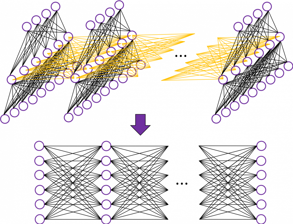
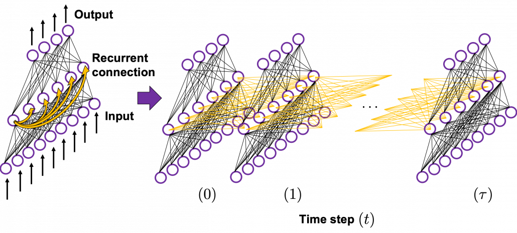
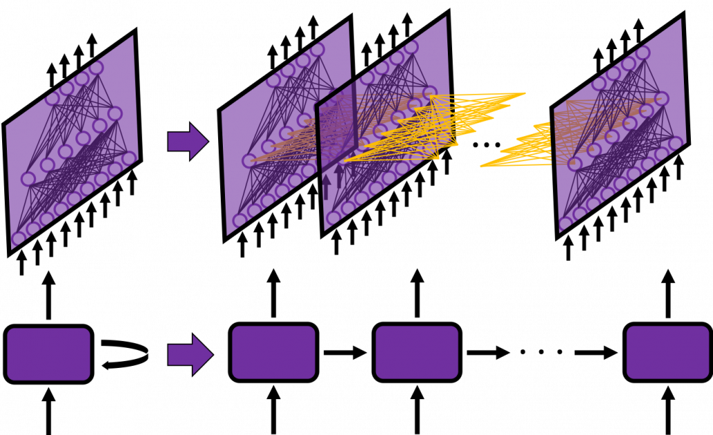
First of all, let’s take a brief look at what I said about the structures of RNNs,  in the first and the second article. A simple RNN is basically densely connected network with a few layers. But the RNN gets an input every time step, and it gives out an output at the time step. Part of information in the middle layer are succeeded to the next time step, and in the next time step, the RNN also gets an input and gives out an output. Therefore, virtually a simple RNN behaves almost the same way as densely connected layers with many layers during forward/back propagation if you focus on its recurrent connections.

That is why simple RNNs suffer from vanishing/exploding gradient problems, where the information exponentially vanishes or explodes when its gradients are multiplied many times through many layers during back propagation. To be exact, I think you need to consider this problem precisely like you can see in this paper. But for now, please at least keep it in mind that when you calculate a gradient of an error function with respect to parameters of simple neural networks, you have to multiply parameters many times like below, and this type of calculation usually leads to vanishing/exploding gradient problem.

LSTM was invented as a way to tackle such problems as I mentioned in the last article.

3. How to display LSTM

I would like you to just go to image search on Google, Bing, or Yahoo!, and type in “LSTM.” I think you will find many figures, but basically LSTM charts are roughly classified into two types: in this article I call them “Space Odyssey type” and “electronic circuit type”, and in conclusion, I highly recommend you to understand LSTM as the “electronic circuit type.”

*I just randomly came up with the terms “Space Odyssey type” and “electronic circuit type” because the former one is used in the paper I mentioned, and the latter one looks like an electronic circuit to me. You do not have to take how I call them seriously.

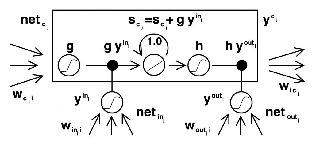
However, not that all the well-made explanations on LSTM use the “electronic circuit type,” and I am sure you sometimes have to understand LSTM as the “space odyssey type.” And the paper “LSTM: A Search Space Odyssey,” which I learned a lot about LSTM from,  also adopts the “Space Odyssey type.”

LSTM architectur visualization

The main reason why I recommend the “electronic circuit type” is that its behaviors look closer to that of simple RNNs, which you would have seen if you read my former articles.

*Behaviors of both of them look different, but of course they are doing the same things.

If you have some understanding on DCL, I think it was not so hard to understand how simple RNNs work because simple RNNs  are mainly composed of linear connections of neurons and weights, whose structures are the same almost everywhere. And basically they had only straightforward linear connections as you can see below.

But from now on, I would like you to give up the ideas that LSTM is composed of connections of neurons like the head image of this article series. If you do that, I think that would be chaotic and I do not want to make a figure of it on Power Point. In short, sooner or later you have to understand equations of LSTM.

4. Forward propagation of LSTM in “electronic circuit type”

*For further understanding of mathematics of LSTM forward/back propagation, I recommend you to download my slides.

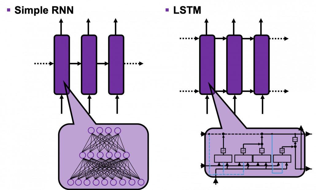
The behaviors of an LSTM block is quite similar to that of a simple RNN block: an RNN block gets an input every time step and gets information from the RNN block of the last time step, via recurrent connections. And the block succeeds information to the next block.

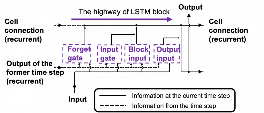
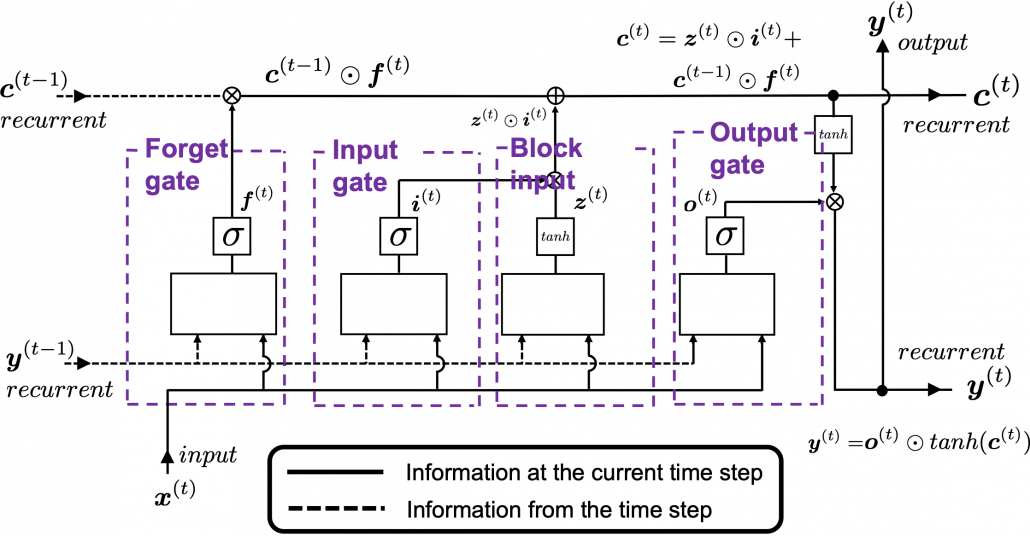
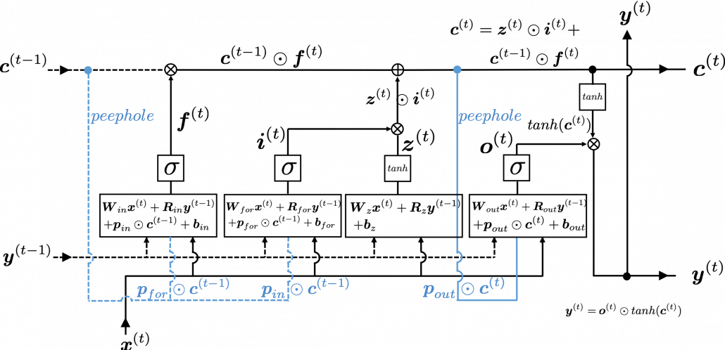
Let’s look at the simplified architecture of  an LSTM block. First of all, you should keep it in mind that LSTM have two streams of information: the one going through all the gates, and the one going through cell connections, the “highway” of LSTM block. For simplicity, we will see the architecture of an LSTM block without peephole connections, the lines in blue. The flow of information through cell connections is relatively uninterrupted. This helps LSTMs to retain information for a long time.

In a LSTM block, the input and the output of the former time step separately go through sections named “gates”: input gate, forget gate, output gate, and block input. The outputs of the forget gate, the input gate, and the block input join the highway of cell connections to renew the value of the cell.

*The small two dots on the cell connections are the “on-ramp” of cell conection highway.

*You would see the terms “input gate,” “forget gate,” “output gate” almost everywhere, but how to call the “block gate” depends on textbooks.

Let’s look at the structure of an LSTM block a bit more concretely. An LSTM block at the time step (t) gets \boldsymbol{y}^{(t-1)}, the output at the last time step,  and \boldsymbol{c}^{(t-1)}, the information of the cell at the time step (t-1), via recurrent connections. The block at time step (t) gets the input \boldsymbol{x}^{(t)}, and it separately goes through each gate, together with \boldsymbol{y}^{(t-1)}. After some calculations and activation, each gate gives out an output. The outputs of the forget gate, the input gate, the block input, and the output gate are respectively \boldsymbol{f}^{(t)}, \boldsymbol{i}^{(t)}, \boldsymbol{z}^{(t)}, \boldsymbol{o}^{(t)}. The outputs of the gates are mixed with \boldsymbol{c}^{(t-1)} and the LSTM block gives out an output \boldsymbol{y}^{(t)}, and gives \boldsymbol{y}^{(t)} and \boldsymbol{c}^{(t)} to the next LSTM block via recurrent connections.

You calculate \boldsymbol{f}^{(t)}, \boldsymbol{i}^{(t)}, \boldsymbol{z}^{(t)}, \boldsymbol{o}^{(t)} as below.

  • \boldsymbol{f}^{(t)}= \sigma(\boldsymbol{W}_{for} \boldsymbol{x}^{(t)} + \boldsymbol{R}_{for} \boldsymbol{y}^{(t-1)} +  \boldsymbol{b}_{for})
  • \boldsymbol{i}^{(t)}=\sigma(\boldsymbol{W}_{in} \boldsymbol{x}^{(t)} + \boldsymbol{R}_{in} \boldsymbol{y}^{(t-1)} + \boldsymbol{b}_{in})
  • \boldsymbol{z}^{(t)}=tanh(\boldsymbol{W}_z \boldsymbol{x}^{(t)} + \boldsymbol{R}_z \boldsymbol{y}^{(t-1)} + \boldsymbol{b}_z)
  • \boldsymbol{o}^{(t)}=\sigma(\boldsymbol{W}_{out} \boldsymbol{x}^{(t)} + \boldsymbol{R}_{out} \boldsymbol{y}^{(t-1)} + \boldsymbol{b}_{out})

*You have to keep it in mind that the equations above do not include peephole connections, which I am going to show with blue lines in the end.

The equations above are quite straightforward if you understand forward propagation of simple neural networks. You add linear products of \boldsymbol{y}^{(t)} and \boldsymbol{c}^{(t)} with different weights in each gate. What makes LSTMs different from simple RNNs is how to mix the outputs of the gates with the cell connections. In order to explain that, I need to introduce a mathematical operator called Hadamard product, which you denote as \odot. This is a very simple operator. This operator produces an elementwise product of two vectors or matrices with identical shape.

With this Hadamar product operator, the renewed cell and the output are calculated as below.

  • \boldsymbol{c}^{(t)} = \boldsymbol{z}^{(t)}\odot \boldsymbol{i}^{(t)} + \boldsymbol{c}^{(t-1)} \odot \boldsymbol{f}^{(t)}
  • \boldsymbol{y}^{(t)} = \boldsymbol{o}^{(t)} \odot tanh(\boldsymbol{c}^{(t)})

The values of \boldsymbol{f}^{(t)}, \boldsymbol{i}^{(t)}, \boldsymbol{z}^{(t)}, \boldsymbol{o}^{(t)} are compressed into the range of [0, 1] or [-1, 1] with activation functions. You can see that the input gate and the block input give new information to the cell. The part \boldsymbol{c}^{(t-1)} \odot \boldsymbol{f}^{(t)} means that the output of the forget gate “forgets” the cell of the last time step by multiplying the values from 0 to 1 elementwise. And the cell \boldsymbol{c}^{(t)} is activated with tanh() and the output of the output gate “suppress” the activated value of \boldsymbol{c}^{(t)}. In other words, the output gatedecides how much information to give out as an output of the LSTM block. The output of every gate depends on the input \boldsymbol{x}^{(t)}, and the recurrent connection \boldsymbol{y}^{(t-1)}. That means an LSTM block learns to forget the cell of the last time step, to renew the cell, and to suppress the output. To describe in an extreme manner, if all the outputs of every gate are always (1, 1, …1)^T, LSTMs forget nothing, retain information of inputs at every time step, and gives out everything. And  if all the outputs of every gate are always (0, 0, …0)^T, LSTMs forget everything, receive no inputs, and give out nothing.

This model has one problem: the outputs of each gate do not directly depend on the information in the cell. To solve this problem, some LSTM models introduce some flows of information from the cell to each gate, which are shown as lines in blue in the figure below.

LSTM inner architecture

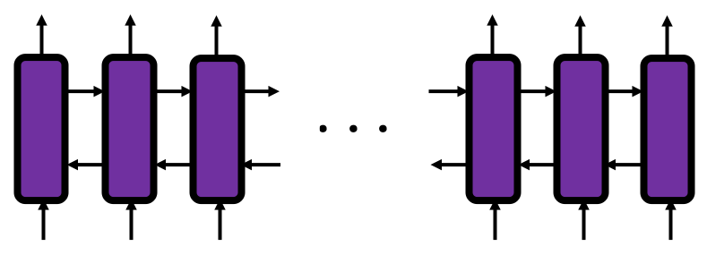
LSTM models, for example the one with or without peephole connection, depend on the library you use, and the model I have showed is one of standard LSTM structure. However no matter how complicated structure of an LSTM block looks, you usually cover it with a black box as below and show its behavior in a very simplified way.

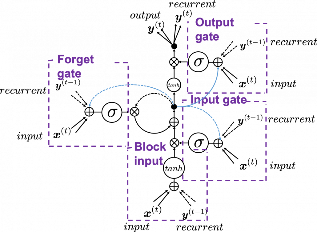
5. Space Odyssey type

I personally think there is no advantages of understanding how LSTMs work with this Space Odyssey type chart, but in several cases you would have to use this type of chart. So I will briefly explain how to look at that type of chart, based on understandings of LSTMs you have gained through this article.

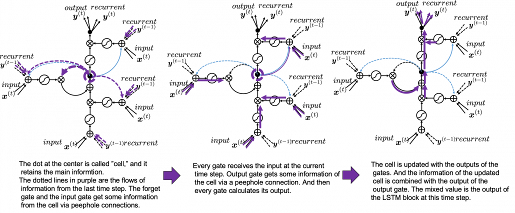
In Space Odyssey type of LSTM chart, at the center is a cell. Electronic circuit type of chart, which shows the flow of information of the cell as an uninterrupted “highway” in an LSTM block. On the other hand, in a Spacey Odyssey type of chart, the information of the cell rotate at the center. And each gate gets the information of the cell through peephole connections,  \boldsymbol{x}^{(t)}, the input at the time step (t) , sand \boldsymbol{y}^{(t-1)}, the output at the last time step (t-1), which came through recurrent connections. In Space Odyssey type of chart, you can more clearly see that the information of the cell go to each gate through the peephole connections in blue. Each gate calculates its output.

Just as the charts you have seen, the dotted line denote the information from the past. First, the information of the cell at the time step (t-1) goes to the forget gate and get mixed with the output of the forget cell In this process the cell is partly “forgotten.” Next, the input gate and the block input are mixed to generate part of new value of the the cell at time step  (t). And the partly “forgotten” \boldsymbol{c}^{(t-1)} goes back to the center of the block and it is mixed with the output of the input gate and the block input. That is how \boldsymbol{c}^{(t)} is renewed. And the value of new cell flow to the top of the chart, being mixed with the output of the output gate. Or you can also say the information of new cell is “suppressed” with the output gate.

I have finished the first four articles of this article series, and finally I am gong to write about back propagation of LSTM in the next article. I have to say what I have written so far is all for the next article, and my long long Power Point slides.


[References]

[1] Klaus Greff, Rupesh Kumar Srivastava, Jan Koutník, Bas R. Steunebrink, Jürgen Schmidhuber, “LSTM: A Search Space Odyssey,” (2017)

[2] Francois Chollet, Deep Learning with Python,(2018), Manning , pp. 202-204

[3] “Sepp Hochreiter receives IEEE CIS Neural Networks Pioneer Award 2021”, Institute of advanced research in artificial intelligence, (2020)
URL: https://www.iarai.ac.at/news/sepp-hochreiter-receives-ieee-cis-neural-networks-pioneer-award-2021/?fbclid=IwAR27cwT5MfCw4Tqzs3MX_W9eahYDcIFuoGymATDR1A-gbtVmDpb8ExfQ87A

[4] Oketani Takayuki, “Machine Learning Professional Series: Deep Learning,” (2015), pp. 120-125
岡谷貴之 著, 「機械学習プロフェッショナルシリーズ 深層学習」, (2015), pp. 120-125

[5] Harada Tatsuya, “Machine Learning Professional Series: Image Recognition,” (2017), pp. 252-257
原田達也 著, 「機械学習プロフェッショナルシリーズ 画像認識」, (2017), pp. 252-257

[6] “Understandable LSTM ~ With the Current Trends,” Qiita, (2015)
「わかるLSTM ~ 最近の動向と共に」, Qiita, (2015)
URL: https://qiita.com/t_Signull/items/21b82be280b46f467d1b

Simple RNN

A brief history of neural nets: everything you should know before learning LSTM

This is not a college course or something on deep learning with strict deadlines for assignments, so let’s take a detour from practical stuff and take a brief look at the history of neural networks.

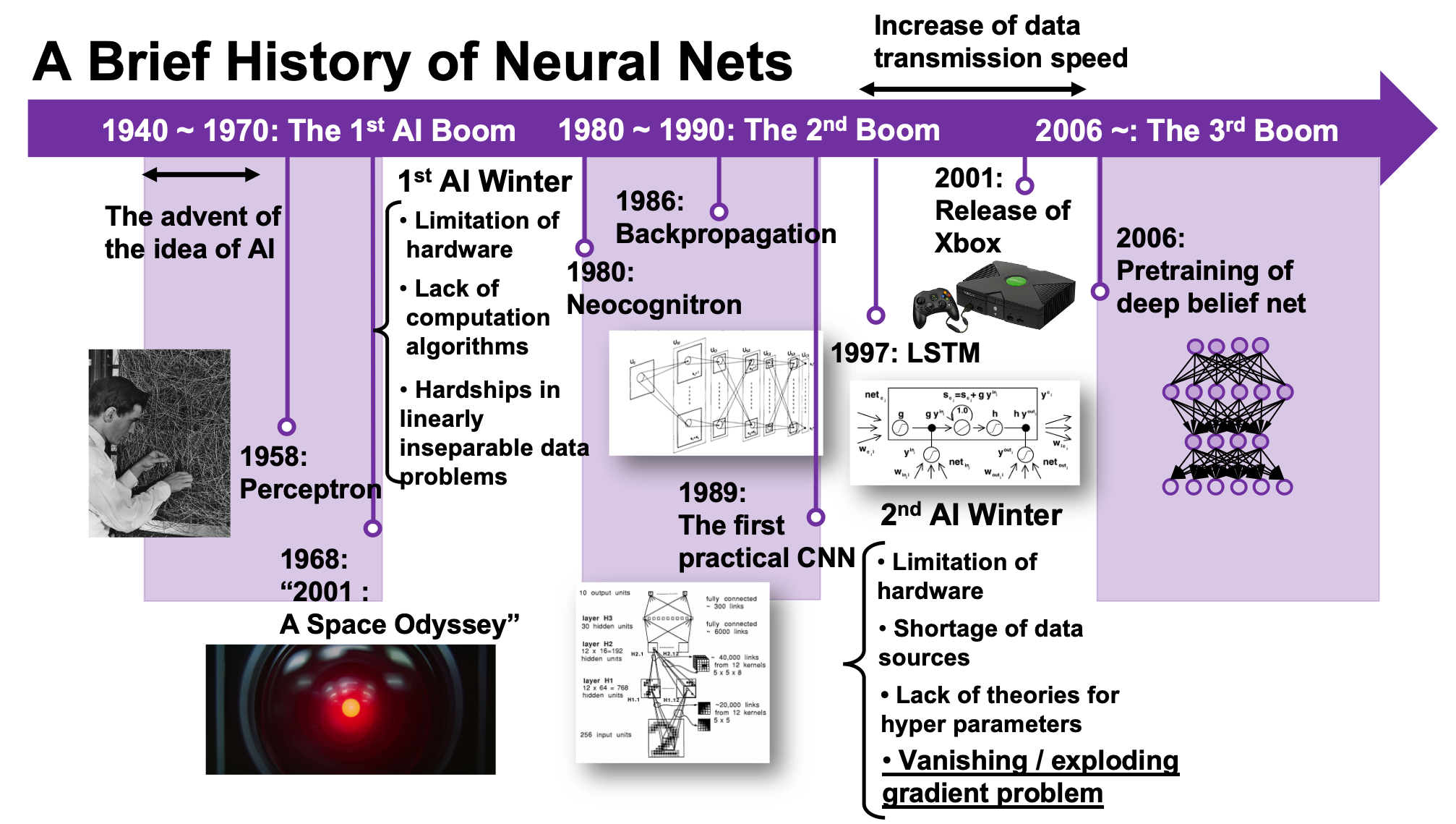
The history of neural networks is also a big topic, which could be so long that I had to prepare another article series. And usually I am supposed to begin such articles with something like “The term ‘AI’ was first used by John McCarthy in Dartmouth conference 1956…” but you can find many of such texts written by people with much more experiences in this field. Therefore I am going to write this article from my point of view, as an intern writing articles on RNN, as a movie buff, and as one of many Japanese men who spent a great deal of childhood with video games.

We are now in the third AI boom, and some researchers say this boom began in 2006. A professor in my university said there we are now in a kind of bubble economy in machine learning/data science industry, but people used to say “Stop daydreaming” to AI researchers. The second AI winter is partly due to vanishing/exploding gradient problem of deep learning. And LSTM was invented as one way to tackle such problems, in 1997.

1, First AI boom

In the first AI boom, I think people were literally “daydreaming.” Even though the applications of machine learning algorithms were limited to simple tasks like playing chess, checker, or searching route of 2d mazes, and sometimes this time is called GOFAI (Good Old Fashioned AI).

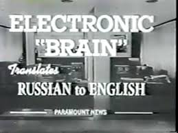
Even today when someone use the term “AI” merely for tasks with neural networks, that amuses me because for me deep learning is just statistically and automatically training neural networks, which are capable of universal approximation, into some classifiers/regressors. Actually the algorithms behind that is quite impressive, but the structure of human brains is much more complicated. The hype of “AI” already started in this first AI boom. Let me take an example of machine translation in this video. In fact the research of machine translation already started in the early 1950s, and of  specific interest in the time was translation between English and Russian due to Cold War. In the first article of this series, I said one of the most famous applications of RNN is machine translation, such as Google Translation, DeepL. They are a type of machine translation called neural machine translation because they use neural networks, especially RNNs. Neural machine translation was an astonishing breakthrough around 2014 in machine translation field. The former major type of machine translation was statistical machine translation, based on statistical language models. And the machine translator in the first AI boom was rule base machine translators, which are more primitive than statistical ones.

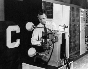
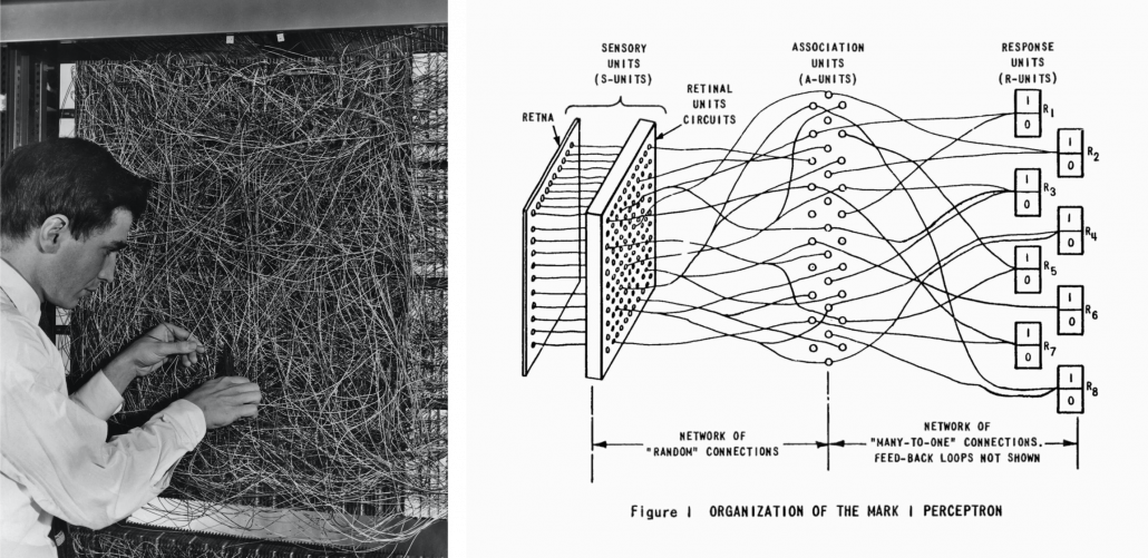
The most remarkable invention in this time was of course perceptron by Frank Rosenblatt. Some people say that this is the first neural network. Even though you can implement perceptron with a-few-line codes in Python, obviously they did not have Jupyter Notebook in those days. The perceptron was implemented as a huge instrument named Mark 1 Perceptron, and it was composed of randomly connected wires. I do not precisely know how it works, but it was a huge effort to implement even the most primitive type of neural networks. They needed to use a big lighting fixture to get a 20*20 pixel image using 20*20 array of cadmium sulphide photocells. The research by Rosenblatt, however, was criticized by Marvin Minsky in his book because perceptrons could only be used for linearly separable data. To make matters worse the criticism prevailed as that more general, multi-layer perceptrons were also not useful for linearly inseparable data (as I mentioned in the first article, multi-layer perceptrons, namely normal neural networks,  can be universal approximators, which have potentials to classify/regress various types of complex data). In case you do not know what “linearly separable” means, imagine that there are data plotted on a piece of paper. If an elementary school kid can draw a border line between two clusters of the data with a ruler and a pencil on the paper, the 2d data is “linearly separable”….

With big disappointments to the research on “electronic brains,” the budget of AI research was reduced and AI research entered its first winter.

I think  the frame problem(1969),  by John McCarthy and Patrick J. Hayes, is also an iconic theory in the end of the first AI boom. This theory is known as a story of creating a robot trying to pull out its battery on a wheeled wagon in a room. The first prototype of the robot, named R1, naively tried to pull out the wagon form the room, and the bomb exploded. The problems was obvious: R1 was not programmed to consider the risks by taking each action, so the researchers made the next prototype named R1D1, which was programmed to consider the potential risks of taking each action. When R1D1 tried to pull out the wagon, it realized the risk of pulling the bomb together with the battery. But soon it started considering all the potential risks, such as the risk of the ceiling falling down, the distance between the wagon and all the walls, and so on, when the bomb exploded. The next problem was also obvious: R1D1 was not programmed to distinguish if the factors are relevant of irrelevant to the main purpose, and the next prototype R2D1 was programmed to do distinguish them. This time, R2D1 started thinking about “whether the factor is  irrelevant to the main purpose,” on every factor measured, and again the bomb exploded. How can we get a perfect AI, R2D2?

The situation of mentioned above is a bit extreme, but it is said AI could also get stuck when it try to take some super simple actions like finding a number in a phone book and make a phone call. It is difficult for an artificial intelligence to decide what is relevant and what is irrelevant, but humans will not get stuck with such simple stuff, and sometimes the frame problem is counted as the most difficult and essential problem of developing AI. But personally I think the original frame problem was unreasonable in that McCarthy, in his attempts to model the real world, was inflexible in his handling of the various equations involved, treating them all with equal weight regardless of the particular circumstances of a situation. Some people say that McCarthy, who was an advocate for AI, also wanted to see the field come to an end, due to its failure to meet the high expectations it once aroused.

Not only the frame problem, but also many other AI-related technological/philosophical problems have been proposed, such as Chinese room (1980), the symbol grounding problem (1990), and they are thought to be as hardships in inventing artificial intelligence, but I omit those topics in this article.

*The name R2D2 did not come from the famous story of frame problem. The story was Daniel Dennett first proposed the story of R2D2 in his paper published in 1984. Star Wars was first released in 1977. It is said that the name R2D2 came from “Reel 2, Dialogue 2,” which George Lucas said while film shooting. And the design of C3PO came from Maria in Metropolis(1927). It is said that the most famous AI duo in movie history was inspired by Tahei and Matashichi in The Hidden Fortress(1958), directed by Kurosawa Akira.

Interestingly, in the end of the first AI boom, 2001: A Space Odyssey, directed by Stanley Kubrick, was released in 1968. Unlike conventional fantasylike AI characters, for example Maria in Metropolis(1927), HAL 9000 was portrayed as a very realistic AI, and the movie already pointed out the risk of AI being insane when it gets some commands from several users. HAL 9000 still has been a very iconic character in AI field. For example when you say some quotes from 2001: A Space Odyssey to Siri you get some parody responses. I also thin you should keep it in mind that in order to make an AI like HAL 9000 come true, for now RNNs would be indispensable in many ways: you would need RNNs for better voice recognition, better conversational system, and for reading lips.

*Just as you cannot understand Monty Python references in Python official tutorials without watching Monty Python and the Holy Grail, you cannot understand many parodies in AI contexts without watching 2001: A Space Odyssey. Even thought the movie had some interview videos with some researchers and some narrations, Stanley Kubrick cut off all the footage and made the movie very difficult to understand. Most people did not or do not understand that it is a movie about aliens who gave homework of coming to Jupiter to human beings.

2, Second AI boom/winter

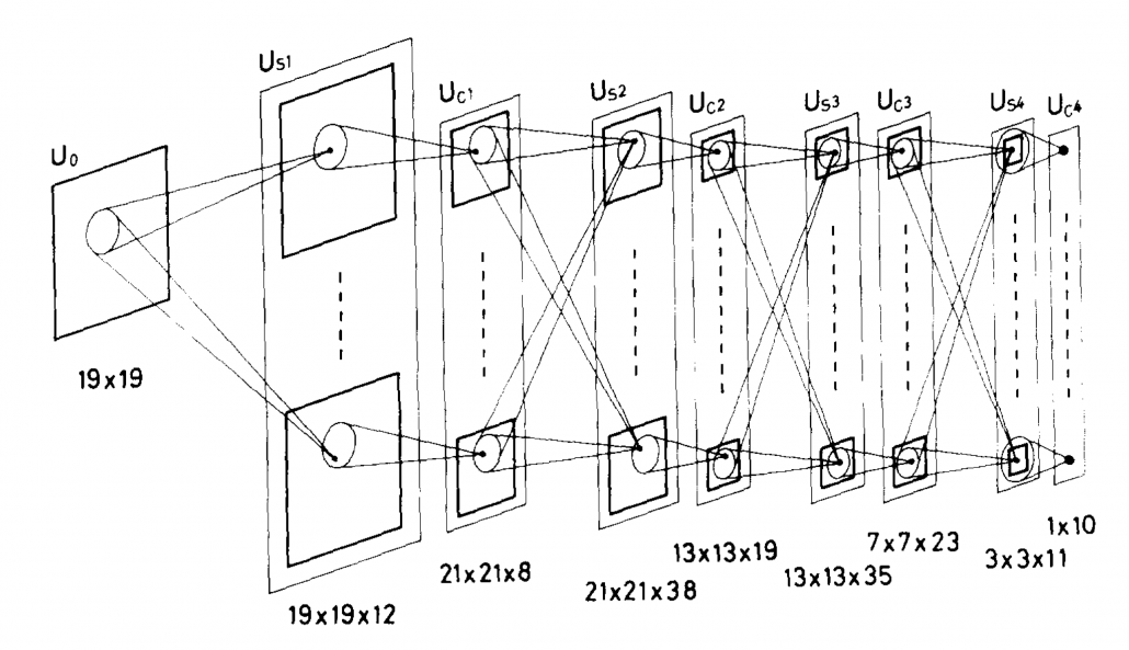
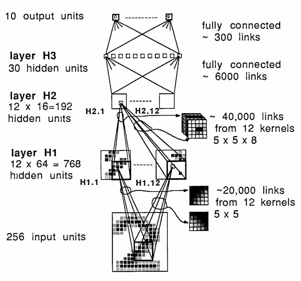
I am not going to write about the second AI boom in detail, but at least you should keep it in mind that convolutional neural network(CNN) is a keyword in this time. Neocognitron, an artificial model of how sight nerves perceive thing, was invented by Kunihiko Fukushima in 1980, and the model is said to be the origin on CNN. And Neocognitron got inspired by the Hubel and Wiesel’s research on sight nerves. In 1989, a group in AT & T Bell Laboratory led by Yann LeCun invented the first practical CNN to read handwritten digit.

Another turning point in this second AI boom was that back propagation algorithm was discovered, and the CNN by LeCun was also trained with back propagation. LeCun made a deep neural networks with some layers in 1998 for more practical uses.

But his research did not gain so much attention like today, because AI research entered its second winter at the beginning of the 1990s, and that was partly due to vanishing/exploding gradient problem of deep learning. People knew that neural networks had potentials of universal approximation, but when they tried to train naively stacked neural nets the gradients, which you need to train neural networks, exponentially increased/decreased. Even though the CNN made by LeCun was the first successful case of “deep” neural nets which did not suffer from the vanishing/exploding gradient problem, deep learning research also stagnated in this time.

The ultimate goal of this article series is to understand LSTM at a more abstract/mathematical level because it is one of the practical RNNs, but the idea of LSTM (Long Short Term Memory) itself was already proposed in 1997 as an RNN algorithm to tackle vanishing gradient problem. (Exploding gradient problem is solved with a technique named gradient clipping, and this is easier than techniques for preventing vanishing gradient problems. I am also going to explain it in the next article.) After that some other techniques like introducing forget gate, peephole connections, were discovered, but basically it took some 20 years till LSTM got attentions like today. The reasons for that is lack of hardware and data sets, and that was also major reasons for the second AI winter.

In the 1990s, the mid of second AI winter, the Internet started prevailing for commercial uses. I think one of the iconic events in this time was the source codes WWW(World Wide Web) were announced in 1993. Some of you might still remember that you little by little became able to transmit more data online in this time. That means people came to get more and more access to various datasets in those days, which is indispensable for machine learning tasks.

After all, we could not get HAL 9000 by the end of 2001, but instead we got Xbox console.

3, Video game industry and GPU

Even though research on neural networks stagnated in the 1990s the same period witnessed an advance in the computation of massive parallel linear transformations, due to their need in fields such as image processing.

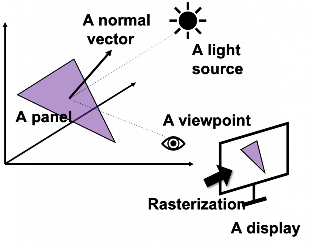
Computer graphics move or rotate in 3d spaces, and that is also linear transformations. When you think about a car moving in a city, it is convenient to place the car, buildings, and other objects on a fixed 3d space. But when you need to make computer graphics of scenes of the city from a view point inside the car, you put a moving origin point in the car and see the city. The spatial information of the city is calculated as vectors from the moving origin point. Of course this is also linear transformations. Of course I am not talking about a dot or simple figures moving in the 3d spaces. Computer graphics are composed of numerous plane panels, and each of them have at least three vertexes, and they move on 3d spaces. Depending on viewpoints, you need project the 3d graphics in 3d spaces on 2d spaces to display the graphics on devices. You need to calculate which part of the panel is projected to which pixel on the display, and that is called rasterization. Plus, in order to get photophotorealistic image, you need to think about how lights from light sources reflect on the panel and projected on the display. And you also have to put some textures on groups of panels. You might also need to change color spaces, which is also linear transformations.

My point is, in short, you really need to do numerous linear transformations in parallel in image processing.

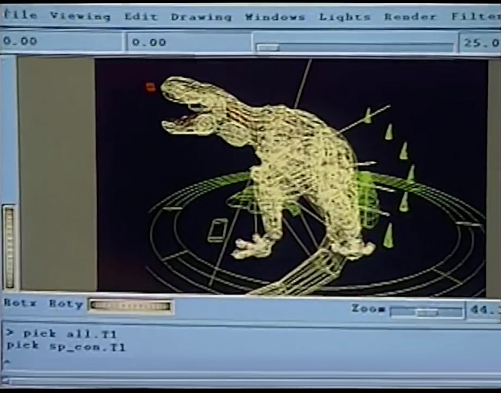
When it comes to the use of CGI in movies,  two pioneer movies were released during this time: Jurassic Park in 1993, and Toy Story in 1995. It is famous that Pixar used to be one of the departments in ILM(Industrial Light and Magic), founded by George Lucas, and Steve Jobs bought the department. Even though the members in Pixar had not even made a long feature film in their lives, after trial and errors, they made the first CGI animated feature movie. On the other hand, in order to acquire funds for the production of Schindler’s List(1993), Steven Spielberg took on Jurassic Park(1993), consequently changing the history of CGI through this “side job.”

*I think you have realized that George Lucas is mentioned almost everywhere in this article. His influences on technologies are not only limited to image processing, but also sound measuring system, nonlinear editing system. Photoshop was also originally developed under his company. I need another article series for this topic, but maybe not in Data Science Blog.

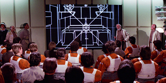
Considering that the first wire-frame computer graphics made and displayed by computers appeared in the scene of displaying the wire frame structure of Death Star in a war room, in Star Wars: A New Hope, the development of CGI was already astonishing at this time. But I think deep learning owe its development more to video game industry.

*I said that the Death Star scene is the first use of graphics made and DISPLAYED by computers, because I have to say one of the first graphics in movie MADE by computer dates back to the legendary title sequence of Vertigo(1958).

When it comes to 3D video games the processing unit has to constantly deal with real time commands from controllers. It is famous that GPU was originally specifically designed for plotting computer graphics. Video game market is the biggest in entertainment industry in general, and it is said that the quality of computer graphics have the strongest correlation with video games sales, therefore enhancing this quality is a priority for the video game console manufacturers.

One good example to see how much video games developed is comparing original Final Fantasy 7 and the remake one. The original one was released in 1997, the same year as when LSTM was invented. And recently  the remake version of Final Fantasy 7 was finally released this year. The original one was also made with very big budget, and it was divided into three CD-ROMs. The original one was also very revolutionary given that the former ones of Final Fantasy franchise were all 2d video retro style video games. But still the computer graphics looks like polygons, and in almost all scenes the camera angle was fixed in the original one. On the other hand the remake one is very photorealistic and you can move the angle of the camera as you want while you play the video game.

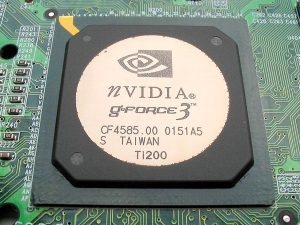
There were also fierce battles by graphic processor manufacturers in computer video game market in the 1990s, but personally I think the release of Xbox console was a turning point in the development of GPU. To be concrete, Microsoft adopted a type of NV20 GPU for Xbox consoles, and that left some room of programmability for developers. The chief architect of NV20, which was released under the brand of GeForce3, said making major changes in the company’s graphic chips was very risky. But that decision opened up possibilities of uses of GPU beyond computer graphics.

I think that the idea of a programmable GPU provided other scientific fields with more visible benefits after CUDA was launched. And GPU gained its position not only in deep learning, but also many other fields including making super computers.

*When it comes to deep learning, even GPUs have strong rivals. TPU(Tensor Processing Unit) made by Google, is specialized for deep learning tasks, and have astonishing processing speed. And FPGA(Field Programmable Gate Array), which was originally invented customizable electronic circuit, proved to be efficient for reducing electricity consumption of deep learning tasks.

*I am not so sure about this GPU part. Processing unit, including GPU is another big topic, that is beyond my capacity to be honest.  I would appreciate it if you could share your view and some references to confirm your opinion, on the comment section or via email.

*If you are interested you should see this video of game fans’ reactions to the announcement of Final Fantasy 7. This is the industry which grew behind the development of deep learning, and many fields where you need parallel computations owe themselves to the nerds who spent a lot of money for video games, including me.

*But ironically the engineers who invented the GPU said they did not play video games simply because they were busy. If you try to study the technologies behind video games, you would not have much time playing them. That is the reality.

We have seen that the in this second AI winter, Internet and GPU laid foundation of the next AI boom. But still the last piece of the puzzle is missing: let’s look at the breakthrough which solved the vanishing /exploding gradient problem of deep learning in the next section.

4, Pretraining of deep belief networks: “The Dawn of Deep Learning”

Some researchers say the invention of pretraining of deep belief network by Geoffrey Hinton was a breakthrough which put an end to the last AI winter. Deep belief networks are different type of networks from the neural networks we have discussed, but their architectures are similar to those of the neural networks. And it was also unknown how to train deep belief nets when they have several layers. Hinton discovered that training the networks layer by layer in advance can tackle vanishing gradient problems. And later it was discovered that you can do pretraining neural networks layer by layer with autoencoders.

*Deep belief network is beyond the scope of this article series. I have to talk about generative models, Boltzmann machine, and some other topics.

The pretraining techniques of neural networks is not mainstream anymore. But I think it is very meaningful to know that major deep learning techniques such as using ReLU activation functions, optimization with Adam, dropout, batch normalization, came up as more effective algorithms for deep learning after the advent of the pretraining techniques, and now we are in the third AI boom.

In the next next article we are finally going to work on LSTM. Specifically, I am going to offer a clearer guide to a well-made paper on LSTM, named “LSTM: A Search Space Odyssey.”

* I make study materials on machine learning, sponsored by DATANOMIQ. I do my best to make my content as straightforward but as precise as possible. I include all of my reference sources. If you notice any mistakes in my materials, including grammatical errors, please let me know (email: yasuto.tamura@datanomiq.de). And if you have any advice for making my materials more understandable to learners, I would appreciate hearing it.
Simple RNN

Simple RNN: the first foothold for understanding LSTM

*In this article “Densely Connected Layers” is written as “DCL,” and “Convolutional Neural Network” as “CNN.”

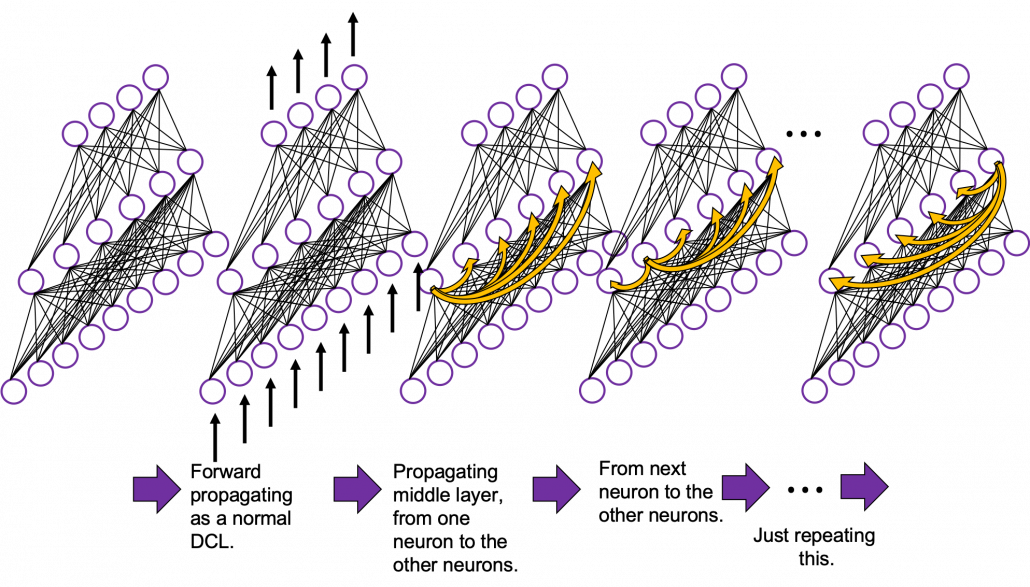
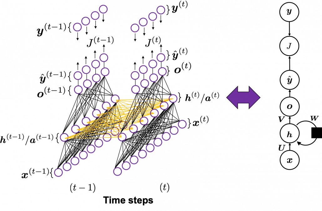
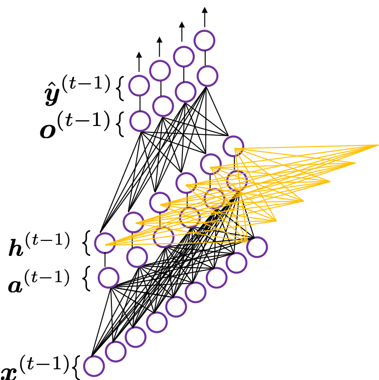
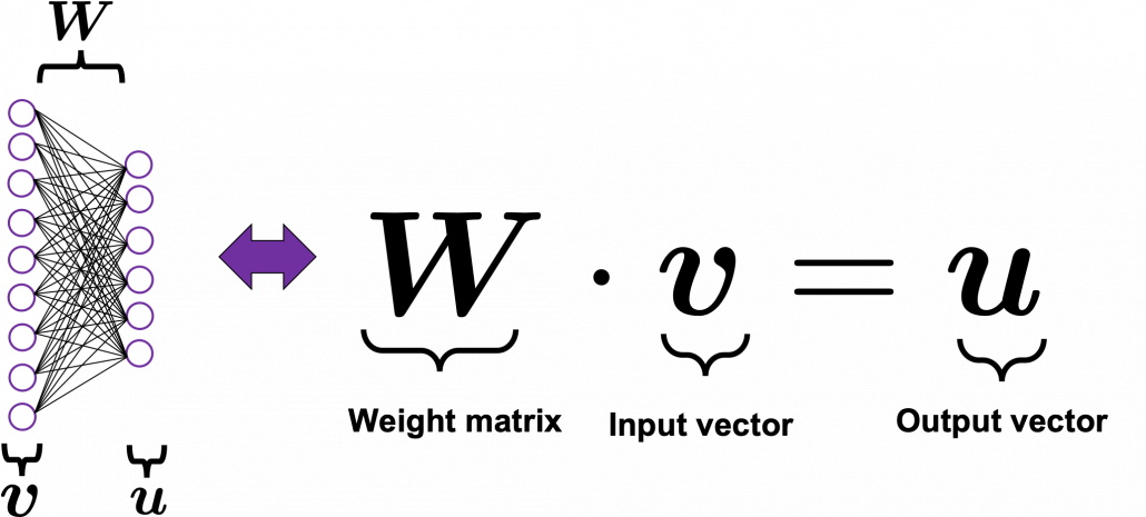
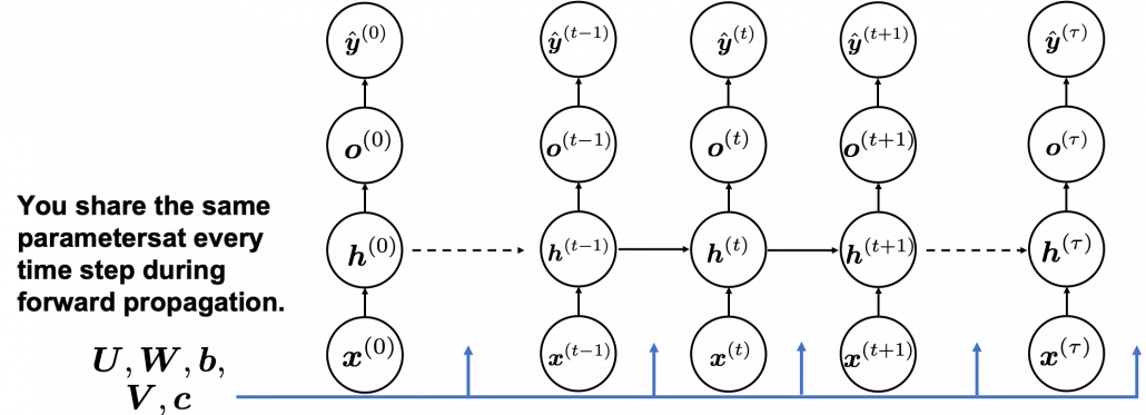
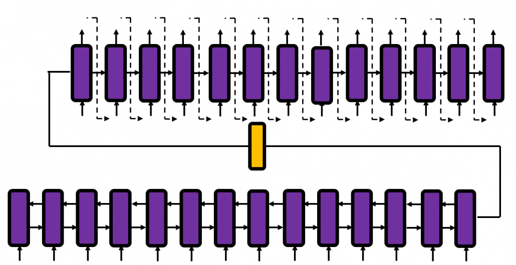
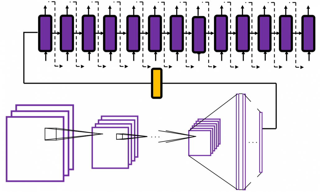
In the last article, I mentioned “When it comes to the structure of RNN, many study materials try to avoid showing that RNNs are also connections of neurons, as well as DCL or CNN.” Even if you manage to understand DCL and CNN, you can be suddenly left behind once you try to understand RNN because it looks like a different field. In the second section of this article, I am going to provide a some helps for more abstract understandings of DCL/CNN , which you need when you read most other study materials.

My explanation on this simple RNN is based on a chapter in a textbook published by Massachusetts Institute of Technology, which is also recommended in some deep learning courses of Stanford University.

First of all, you should keep it in mind that simple RNN are not useful in many cases, mainly because of vanishing/exploding gradient problem, which I am going to explain in the next article. LSTM is one major type of RNN used for tackling those problems. But without clear understanding forward/back propagation of RNN, I think many people would get stuck when they try to understand how LSTM works, especially during its back propagation stage. If you have tried climbing the mountain of understanding LSTM, but found yourself having to retreat back to the foot, I suggest that you read through this article on simple RNNs. It should help you to gain a solid foothold, and you would be ready for trying to climb the mountain again.

*This article is the second article of “A gentle introduction to the tiresome part of understanding RNN.”

1, A brief review on back propagation of DCL.

Simple RNNs are straightforward applications of DCL, but if you do not even have any ideas on DCL forward/back propagation, you will not be able to understand this article. If you more or less understand how back propagation of DCL works, you can skip this first section.

Deep learning is a part of machine learning. And most importantly, whether it is classical machine learning or deep learning, adjusting parameters is what machine learning is all about. Parameters mean elements of functions except for variants. For example when you get a very simple function f(x)=a + bx + cx^2 + dx^3, then x is a variant, and a, b, c, d are parameters. In case of classical machine learning algorithms, the number of those parameters are very limited because they were originally designed manually. Such functions for classical machine learning is useful for features found by humans, after trial and errors(feature engineering is a field of finding such effective features, manually). You adjust those parameters based on how different the outputs(estimated outcome of classification/regression) are from supervising vectors(the data prepared to show ideal answers).

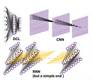
In the last article I said neural networks are just mappings, whose inputs are vectors, matrices, or sequence data. In case of DCLs, inputs are vectors. Then what’s the number of parameters ? The answer depends on the the number of neurons and layers. In the example of DCL at the right side, the number of the connections of the neurons is the number of parameters(Would you like to try to count them? At least I would say “No.”). Unlike classical machine learning you no longer need to do feature engineering, but instead you need to design networks effective for each task and adjust a lot of parameters.

*I think the hype of AI comes from the fact that neural networks find features automatically. But the reality is difficulty of feature engineering was just replaced by difficulty of designing proper neural networks.

It is easy to imagine that you need an efficient way to adjust those parameters, and the method is called back propagation (or just backprop). As long as it is about DCL backprop, you can find a lot of well-made study materials on that, so I am not going to cover that topic precisely in this article series. Simply putting, during back propagation, in order to adjust parameters of a layer you need errors in the next layer. And in order calculate the errors of the next layer, you need errors in the next next layer.

*You should not think too much about what the “errors” exactly mean. Such “errors” are defined in this context, and you will see why you need them if you actually write down all the mathematical equations behind backprops of DCL.

The red arrows in the figure shows how errors of all the neurons in a layer propagate backward to a neuron in last layer. The figure shows only some sets of such errors propagating backward, but in practice you have to think about all the combinations of such red arrows in the whole back propagation(this link would give you some ideas on how DCLs work).

These points are minimum prerequisites for continuing reading this  RNN this article. But if you are planning to understand RNN forward/back propagation at  an abstract/mathematical level that you can read academic papers,  I highly recommend you to actually write down all the equations of DCL backprop. And if possible you should try to implement backprop of three-layer DCL.

2, Forward propagation of simple RNN

In fact the simple RNN which we are going to look at in this article has only three layers. From now on imagine that inputs of RNN come from the bottom and outputs go up. But RNNs have to keep information of earlier times steps during upcoming several time steps because as I mentioned in the last article RNNs are used for sequence data, the order of whose elements is important. In order to do that, information of the neurons in the middle layer of RNN propagate forward to the middle layer itself. Therefore in one time step of forward propagation of RNN, the input at the time step propagates forward as normal DCL, and the RNN gives out an output at the time step. And information of one neuron in the middle layer propagate forward to the other neurons like yellow arrows in the figure. And the information in the next neuron propagate forward to the other neurons, and this process is repeated. This is called recurrent connections of RNN.

*To be exact we are just looking at a type of recurrent connections. For example Elman RNNs have simpler recurrent connections. And recurrent connections of LSTM are more complicated.

Whether it is a simple one or not, basically RNN repeats this process of getting an input at every time step, giving out an output, and making recurrent connections to the RNN itself. But you need to keep the values of activated neurons at every time step, so virtually you need to consider the same RNNs duplicated for several time steps like the figure below. This is the idea of unfolding RNN. Depending on contexts, the whole unfolded DCLs with recurrent connections is also called an RNN.

In many situations, RNNs are simplified as below. If you have read through this article until this point, I bet you gained some better understanding of RNNs, so you should little by little get used to this more abstract, blackboxed  way of showing RNN.

You have seen that you can unfold an RNN, per time step. From now on I am going to show the simple RNN in a simpler way,  based on the MIT textbook which I recomment. The figure below shows how RNN propagate forward during two time steps (t-1), (t).

The input \boldsymbol{x}^{(t-1)}at time step(t-1) propagate forward as a normal DCL, and gives out the output \hat{\boldsymbol{y}} ^{(t)} (The notation on the \boldsymbol{y} ^{(t)} is called “hat,” and it means that the value is an estimated value. Whatever machine learning tasks you work on, the outputs of the functions are just estimations of ideal outcomes. You need to adjust parameters for better estimations. You should always be careful whether it is an actual value or an estimated value in the context of machine learning or statistics). But the most important parts are the middle layers.

*To be exact I should have drawn the middle layers as connections of two layers of neurons like the figure at the right side. But I made my figure closer to the chart in the MIT textbook, and also most other study materials show the combinations of the two neurons before/after activation as one neuron.

\boldsymbol{a}^{(t)} is just linear summations of \boldsymbol{x}^{(t)} (If you do not know what “linear summations” mean, please scroll this page a bit), and \boldsymbol{h}^{(t)} is a combination of activated values of \boldsymbol{a}^{(t)} and linear summations of \boldsymbol{h}^{(t-1)} from the last time step, with recurrent connections. The values of \boldsymbol{h}^{(t)} propagate forward in two ways. One is normal DCL forward propagation to \hat{\boldsymbol{y}} ^{(t)} and \boldsymbol{o}^{(t)}, and the other is recurrent connections to \boldsymbol{h}^{(t+1)} .

These are equations for each step of forward propagation.

  • \boldsymbol{a}^{(t)} = \boldsymbol{b} + \boldsymbol{W} \cdot \boldsymbol{h}^{(t-1)} + \boldsymbol{U} \cdot \boldsymbol{x}^{(t)}
  • \boldsymbol{h}^{(t)}= g(\boldsymbol{a}^{(t)})
  • \boldsymbol{o}^{(t)} = \boldsymbol{c} + \boldsymbol{V} \cdot \boldsymbol{h}^{(t)}
  • \hat{\boldsymbol{y}} ^{(t)} = f(\boldsymbol{o}^{(t)})

*Please forgive me for adding some mathematical equations on this article even though I pledged not to in the first article. You can skip the them, but for some people it is on the contrary more confusing if there are no equations. In case you are allergic to mathematics, I prescribed some treatments below.

*Linear summation is a type of weighted summation of some elements. Concretely, when you have a vector \boldsymbol{x}=(x_0, x_1, x_2), and weights \boldsymbol{w}=(w_0,w_1, w_2), then \boldsymbol{w}^T \cdot \boldsymbol{x} = w_0 \cdot x_0 + w_1 \cdot x_1 +w_2 \cdot x_2 is a linear summation of \boldsymbol{x}, and its weights are \boldsymbol{w}.

*When you see a product of a matrix and a vector, for example a product of \boldsymbol{W} and \boldsymbol{v}, you should clearly make an image of connections between two layers of a neural network. You can also say each element of \boldsymbol{u}} is a linear summations all the elements of \boldsymbol{v}} , and \boldsymbol{W} gives the weights for the summations.

A very important point is that you share the same parameters, in this case \boldsymbol{\theta \in \{\boldsymbol{U}, \boldsymbol{W}, \boldsymbol{b}, \boldsymbol{V}, \boldsymbol{c} \}}, at every time step. 

And you are likely to see this RNN in this blackboxed form.

3, The steps of back propagation of simple RNN

In the last article, I said “I have to say backprop of RNN, especially LSTM (a useful and mainstream type or RNN), is a monster of chain rules.” I did my best to make my PowerPoint on LSTM backprop straightforward. But looking at it again, the LSTM backprop part still looks like an electronic circuit, and it requires some patience from you to understand it. If you want to understand LSTM at a more mathematical level, understanding the flow of simple RNN backprop is indispensable, so I would like you to be patient while understanding this step (and you have to be even more patient while understanding LSTM backprop).

This might be a matter of my literacy, but explanations on RNN backprop are very frustrating for me in the points below.

  • Most explanations just show how to calculate gradients at each time step.
  • Most study materials are visually very poor.
  • Most explanations just emphasize that “errors are back propagating through time,” using tons of arrows, but they lack concrete instructions on how actually you renew parameters with those errors.

If you can relate to the feelings I mentioned above, the instructions from now on could somewhat help you. And I am going to share some study materials on simple RNNs in an external link so that you can gain a clear and mathematical understanding on how simple RNNs work.

Backprop of RNN , as long as you are thinking about simple RNNs, is not so different from that of DCLs. But you have to be careful about the meaning of errors in the context of RNN backprop. Back propagation through time (BPTT) is one of the major methods for RNN backprop, and I am sure most textbooks explain BPTT. But most study materials just emphasize that you need errors from all the time steps, and I think that is very misleading and confusing.

You need all the gradients to adjust parameters, but you do not necessarily need all the errors to calculate those gradients. Gradients in the context of machine learning mean partial derivatives of error functions (in this case J) with respect to certain parameters, and mathematically a gradient of J with respect to \boldsymbol{\theta \in \{\boldsymbol{U}, \boldsymbol{W}, \boldsymbol{b}^{(t)}, \boldsymbol{V}, \boldsymbol{c} \}}is denoted as ( \frac{\partial J}{\partial \boldsymbol{\theta}}  ). And another confusing point in many textbooks, including the MIT one, is that they give an impression that parameters depend on time steps. For example some study materials use notations like \frac{\partial J}{\partial \boldsymbol{\theta}^{(t)}}, and I think this gives an impression that this is a gradient with respect to the parameters at time step (t). In my opinion this gradient rather should be written as ( \frac{\partial J}{\partial \boldsymbol{\theta}} )^{(t)} . But many study materials denote gradients of those errors in the former way, so from now on let me use the notations which you can see in the figures in this article.

In order to calculate the gradient \frac{\partial J}{\partial \boldsymbol{x}^{(t)}} you need errors from time steps s (s \geq t) \quad (as you can see in the figure, in order to calculate a gradient in a colored frame, you need all the errors in the same color).

*Another confusing point is that the \frac{\partial J}{\partial \boldsymbol{\ast ^{(t)}}}, \boldsymbol{\ast} \in \{\boldsymbol{a}^{(t)}, \boldsymbol{h}^{(t)}, \boldsymbol{o}^{(t)}, \dots \} are correct notations, because \boldsymbol{\ast} are values of neurons after forward propagation. They depend on time steps, and these are very values which I have been calling “errors.” That is why parameters do not depend on time steps, whereas errors depend on time steps.

As I mentioned before, you share the same parameters at every time step. Again, please do not assume that parameters are different from time step to time step. It is gradients/errors (you need errors to calculate gradients) which depend on time step. And after calculating errors at every time step, you can finally adjust parameters one time, and that’s why this is called “back propagation through time.” (It is easy to imagine that this method can be very inefficient. If the input is the whole text on a Wikipedia link, you need to input all the sentences in the Wikipedia text to renew parameters one time. To solve this problem there is a backprop method named “truncated BPTT,” with which you renew parameters based on a part of a text. )

And after calculating those gradients \frac{\partial J}{\partial \boldsymbol{\theta}^{(t)}} you can take a summation of them: \frac{\partial J}{\partial \boldsymbol{\theta}}=\sum_{t=0}^{t=\tau}{\frac{\partial J}{\partial \boldsymbol{\theta}^{(t)}}}. With this gradient \frac{\partial J}{\partial \boldsymbol{\theta}} , you can finally renew the value of \boldsymbol{\theta} one time.

At the beginning of this article I mentioned that simple RNNs are no longer for practical uses, and that comes from exploding/vanishing problem of RNN. This problem was one of the reasons for the AI winter which lasted for some 20 years. In the next article I am going to write about LSTM, a fancier type of RNN, in the context of a history of neural network history.

* I make study materials on machine learning, sponsored by DATANOMIQ. I do my best to make my content as straightforward but as precise as possible. I include all of my reference sources. If you notice any mistakes in my materials, including grammatical errors, please let me know (email: yasuto.tamura@datanomiq.de). And if you have any advice for making my materials more understandable to learners, I would appreciate hearing it.
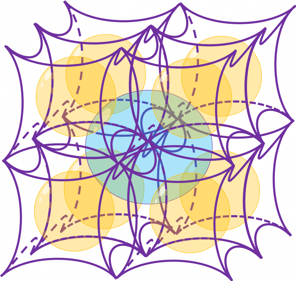
Simple RNN

Prerequisites for understanding RNN at a more mathematical level

Writing the A gentle introduction to the tiresome part of understanding RNN Article Series on recurrent neural network (RNN) is nothing like a creative or ingenious idea. It is quite an ordinary topic. But still I am going to write my own new article on this ordinary topic because I have been frustrated by lack of sufficient explanations on RNN for slow learners like me.

I think many of readers of articles on this website at least know that RNN is a type of neural network used for AI tasks, such as time series prediction, machine translation, and voice recognition. But if you do not understand how RNNs work, especially during its back propagation, this blog series is for you.

After reading this articles series, I think you will be able to understand RNN in more mathematical and abstract ways. But in case some of the readers are allergic or intolerant to mathematics, I tried to use as little mathematics as possible.

Ideal prerequisite knowledge:

  • Some understanding on densely connected layers (or fully connected layers, multilayer perception) and how their forward/back propagation work.
  •  Some understanding on structure of Convolutional Neural Network.

*In this article “Densely Connected Layers” is written as “DCL,” and “Convolutional Neural Network” as “CNN.”

1, Difficulty of Understanding RNN

I bet a part of difficulty of understanding RNN comes from the variety of its structures. If you search “recurrent neural network” on Google Image or something, you will see what I mean. But that cannot be helped because RNN enables a variety of tasks.

Another major difficulty of understanding RNN is understanding its back propagation algorithm. I think some of you found it hard to understand chain rules in calculating back propagation of densely connected layers, where you have to make the most of linear algebra. And I have to say backprop of RNN, especially LSTM, is a monster of chain rules. I am planing to upload not only a blog post on RNN backprop, but also a presentation slides with animations to make it more understandable, in some external links.

In order to avoid such confusions, I am going to introduce a very simplified type of RNN, which I call a “simple RNN.” The RNN displayed as the head image of this article is a simple RNN.

2, How Neurons are Connected

    \begin{equation*}   1 = 3 - 2 \end{equation*}

How to connect neurons and how to activate them is what neural networks are all about. Structures of those neurons are easy to grasp as long as that is about DCL or CNN. But when it comes to the structure of RNN, many study materials try to avoid showing that RNNs are also connections of neurons, as well as DCL or CNN(*If you are not sure how neurons are connected in CNN, this link should be helpful. Draw a random digit in the square at the corner.). In fact the structure of RNN is also the same, and as long as it is a simple RNN, and it is not hard to visualize its structure.

Even though RNN is also connections of neurons, usually most RNN charts are simplified, using blackboxes. In case of simple RNN, most study material would display it as the chart below.

But that also cannot be helped because fancier RNN have more complicated connections of neurons, and there are no longer advantages of displaying RNN as connections of neurons, and you would need to understand RNN in more abstract way, I mean, as you see in most of textbooks.

I am going to explain details of simple RNN in the next article of this series.

3, Neural Networks as Mappings

If you still think that neural networks are something like magical spider webs or models of brain tissues, forget that. They are just ordinary mappings.

If you have been allergic to mathematics in your life, you might have never heard of the word “mapping.” If so, at least please keep it in mind that the equation y=f(x), which most people would have seen in compulsory education, is a part of mapping. If you get a value x, you get a value y corresponding to the x.

But in case of deep learning, x is a vector or a tensor, and it is denoted with \boldsymbol{x} . If you have never studied linear algebra , imagine that a vector is a column of Excel data (only one column), a matrix is a sheet of Excel data (with some rows and columns), and a tensor is some sheets of Excel data (each sheet does not necessarily contain only one column.)

CNNs are mainly used for image processing, so their inputs are usually image data. Image data are in many cases (3, hight, width) tensors because usually an image has red, blue, green channels, and the image in each channel can be expressed as a hight*width matrix (the “height” and the “width” are number of pixels, so they are discrete numbers).

The convolutional part of CNN (which I call “feature extraction part”) maps the tensors to a vector, and the last part is usually DCL, which works as classifier/regressor. At the end of the feature extraction part, you get a vector. I call it a “semantic vector” because the vector has information of “meaning” of the input image. In this link you can see maps of pictures plotted depending on the semantic vector. You can see that even if the pictures are not necessarily close pixelwise, they are close in terms of the “meanings” of the images.

In the example of a dog/cat classifier introduced by François Chollet, the developer of Keras, the CNN maps (3, 150, 150) tensors to 2-dimensional vectors, (1, 0) or (0, 1) for (dog, cat).

Wrapping up the points above, at least you should keep two points in mind: first, DCL is a classifier or a regressor, and CNN is a feature extractor used for image processing. And another important thing is, feature extraction parts of CNNs map images to vectors which are more related to the “meaning” of the image.

Importantly, I would like you to understand RNN this way. An RNN is also just a mapping.

*I recommend you to at least take a look at the beautiful pictures in this link. These pictures give you some insight into how CNN perceive images.

4, Problems of DCL and CNN, and needs for RNN

Taking an example of RNN task should be helpful for this topic. Probably machine translation is the most famous application of RNN, and it is also a good example of showing why DCL and CNN are not proper for some tasks. Its algorithms is out of the scope of this article series, but it would give you a good insight of some features of RNN. I prepared three sentences in German, English, and Japanese, which have the same meaning. Assume that each sentence is divided into some parts as shown below and that each vector corresponds to each part. In machine translation we want to convert a set of the vectors into another set of vectors.

Then let’s see why DCL and CNN are not proper for such task.

  • The input size is fixed: In case of the dog/cat classifier I have mentioned, even though the sizes of the input images varies, they were first molded into (3, 150, 150) tensors. But in machine translation, usually the length of the input is supposed to be flexible.
  • The order of inputs does not mater: In case of the dog/cat classifier the last section, even if the input is “cat,” “cat,” “dog” or “dog,” “cat,” “cat” there’s no difference. And in case of DCL, the network is symmetric, so even if you shuffle inputs, as long as you shuffle all of the input data in the same way, the DCL give out the same outcome . And if you have learned at least one foreign language, it is easy to imagine that the orders of vectors in sequence data matter in machine translation.

*It is said English language has phrase structure grammar, on the other hand Japanese language has dependency grammar. In English, the orders of words are important, but in Japanese as long as the particles and conjugations are correct, the orders of words are very flexible. In my impression, German grammar is between them. As long as you put the verb at the second position and the cases of the words are correct, the orders are also relatively flexible.

5, Sequence Data

We can say DCL and CNN are not useful when you want to process sequence data. Sequence data are a type of data which are lists of vectors. And importantly, the orders of the vectors matter. The number of vectors in sequence data is usually called time steps. A simple example of sequence data is meteorological data measured at a spot every ten minutes, for instance temperature, air pressure, wind velocity, humidity. In this case the data is recorded as 4-dimensional vector every ten minutes.

But this “time step” does not necessarily mean “time.” In case of natural language processing (including machine translation), which you I mentioned in the last section, the numberings of each vector denoting each part of sentences are “time steps.”

And RNNs are mappings from a sequence data to another sequence data.

*At least I found a paper on the RNN’s capability of universal approximation on many-to-one RNN task. But I have not found any papers on universal approximation of many-to-many RNN tasks. Please let me know if you find any clue on whether such approximation is possible. I am desperate to know that. 

6, Types of RNN Tasks

RNN tasks can be classified into some types depending on the lengths of input/output sequences (the “length” means the times steps of input/output sequence data).

If you want to predict the temperature in 24 hours, based on several time series data points in the last 96 hours, the task is many-to-one. If you sample data every ten minutes, the input size is 96*6=574 (the input data is a list of 574 vectors), and the output size is 1 (which is a value of temperature). Another example of many-to-one task is sentiment classification. If you want to judge whether a post on SNS is positive or negative, the input size is very flexible (the length of the post varies.) But the output size is one, which is (1, 0) or (0, 1), which denotes (positive, negative).

*The charts in this section are simplified model of RNN used for each task. Please keep it in mind that they are not 100% correct, but I tried to make them as exact as possible compared to those in other study materials.

Music/text generation can be one-to-many tasks. If you give the first sound/word you can generate a phrase.

Next, let’s look at many-to-many tasks. Machine translation and voice recognition are likely to be major examples of many-to-many tasks, but here name entity recognition seems to be a proper choice. Name entity recognition is task of finding proper noun in a sentence . For example if you got two sentences “He said, ‘Teddy bears on sale!’ ” and ‘He said, “Teddy Roosevelt was a great president!” ‘ judging whether the “Teddy” is a proper noun or a normal noun is name entity recognition.

Machine translation and voice recognition, which are more popular, are also many-to-many tasks, but they use more sophisticated models. In case of machine translation, the inputs are sentences in the original language, and the outputs are sentences in another language. When it comes to voice recognition, the input is data of air pressure at several time steps, and the output is the recognized word or sentence. Again, these are out of the scope of this article but I would like to introduce the models briefly.

Machine translation uses a type of RNN named sequence-to-sequence model (which is often called seq2seq model). This model is also very important for other natural language processes tasks in general, such as text summarization. A seq2seq model is divided into the encoder part and the decoder part. The encoder gives out a hidden state vector and it used as the input of the decoder part. And decoder part generates texts, using the output of the last time step as the input of next time step.

Voice recognition is also a famous application of RNN, but it also needs a special type of RNN.

*To be honest, I don’t know what is the state-of-the-art voice recognition algorithm. The example in this article is a combination of RNN and a collapsing function made using Connectionist Temporal Classification (CTC). In this model, the output of RNN is much longer than the recorded words or sentences, so a collapsing function reduces the output into next output with normal length.

You might have noticed that RNNs in the charts above are connected in both directions. Depending on the RNN tasks you need such bidirectional RNNs.  I think it is also easy to imagine that such networks are necessary. Again, machine translation is a good example.

And interestingly, image captioning, which enables a computer to describe a picture, is one-to-many-task. As the output is a sentence, it is easy to imagine that the output is “many.” If it is a one-to-many task, the input is supposed to be a vector.

Where does the input come from? I told you that I was obsessed with the beauty of the last vector of the feature extraction part of CNN. Surprisingly the the “beautiful” vector, which I call a “semantic vector” is the input of image captioning task (after some transformations, depending on the network models).

I think this articles includes major things you need to know as prerequisites when you want to understand RNN at more mathematical level. In the next article, I would like to explain the structure of a simple RNN, and how it forward propagate.

* I make study materials on machine learning, sponsored by DATANOMIQ. I do my best to make my content as straightforward but as precise as possible. I include all of my reference sources. If you notice any mistakes in my materials, please let me know (email: yasuto.tamura@datanomiq.de). And if you have any advice for making my materials more understandable to learners, I would appreciate hearing it.
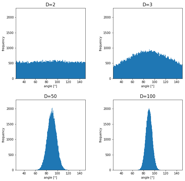
Deep Learning World – Virtual Edition 2020!

DEEP LEARNING WORLD 2020

Virtual Edition, May 11-12, 2020

The premier conference covering the
commercial deployment of deep learning

Deep Learning is no longer the cool new discipline. Instead it has become another tool in the toolbox of the data scientist – but a very important one! Without RNN, CNN etc. many applications that make our daily life better or help us to improve our business wouldn’t be possible. Take for example the German Federal State NRW: they are using neural networks to detect child pornography. Other organizations use it to detect cancer, translate text or inspect machines. It’s also important to understand how Deep Learning sits alongside traditional machine learning methods. As an expert you should know when and how to apply different methods for different applications. At the Deep Learning World conference, you will learn from other practitioners why they decided for a deep, transfer or reinforcement learning approach, what the analytical and technical but also organisational and economic challenges were and how they solved them. Take this opportunity and visit the two-day event to broaden your knowledge, deepen your understanding and discuss your questions with other Deep Learning experts – see you virtually in May 2020!

Why should you participate?

We will provide a live-streamed virtual version of deep learning on 11-12 May, 2020: you will be able to attend sessions and to interact and connect with the speakers and fellow members of the data science community including sponsors and exhibitors from your home or your office.

What about the workshops?

The workshops will also be held virtually on the planned date:
13 May, 2020.

Don’t have a ticket yet?

It‘s not too late to join the data science community.
Register by 10 May to receive access to the livestream and recordings.

REGISTER HERE

We’re looking forward to see you – virtually!

This year the Deep Learning World runs alongside with the Predictive Analytics World for Healthcare and Predictive Analytics World for Industry 4.0.

Predictive Analytics World for Industry 4.0

Difficult times call for creative measures

Predictive Analytics World for Industry 4.0 will go virtual and you still have time to join us!

What do you have in store for me?

We will provide a live-streamed virtual version of PAW Industry 4.0 Munich 2020 on 11-12 May, 2020: you will be able to attend sessions and to interact and connect with the speakers and fellow members of the data science community including sponsors and exhibitors from your home or your office.

What about the workshops?

The workshops will also be held virtually on the planned date:
13 May, 2020.

Get a complimentary virtual sneak preview!

If you would like to join us for a virtual sneak preview of the workshop „Data Thinking“ on Thursday, April 16, so you can familiarise yourself with the quality of the virtual edition of both conference and workshops and how the interaction with speakers and attendees works, please send a request to registration@risingmedia.com.

Don’t have a ticket yet?

It‘s not too late to join the data science community.
Register by 10 May to receive access to the livestream and recordings.

REGISTER HERE

We’re looking forward to see you – virtually!

This year Predictive Analytics World for Industry 4.0 runs alongside Deep Learning World and Predictive Analytics World for Healthcare.

Visual Question Answering with Keras – Part 2: Making Computers Intelligent to answer from images

Making Computers Intelligent to answer from images

This is my second blog on Visual Question Answering, in the last blog, I have introduced to VQA, available datasets and some of the real-life applications of VQA. If you have not gone through then I would highly recommend you to go through it. Click here for more details about it.

In this blog post, I will walk through the implementation of VQA in Keras.

You can download the dataset from here: https://visualqa.org/index.html. All my experiments were performed with VQA v2 and I have used a very tiny subset of entire dataset i.e all samples for training and testing from the validation set.

Table of contents:

  1. Preprocessing Data
  2. Process overview for VQA
  3. Data Preprocessing – Images
  4. Data Preprocessing through the spaCy library- Questions
  5. Model Architecture
  6. Defining model parameters
  7. Evaluating the model
  8. Final Thought
  9. References

NOTE: The purpose of this blog is not to get the state-of-art performance on VQA. But the idea is to get familiar with the concept. All my experiments were performed with the validation set only.

Full code on my Github here.


1. Preprocessing Data:

If you have downloaded the dataset then the question and answers (called as annotations) are in JSON format. I have provided the code to extract the questions, annotations and other useful information in my Github repository. All extracted information is stored in .txt file format. After executing code the preprocessing directory will have the following structure.

All text files will be used for training.


2. Process overview for VQA:

As we have discussed in previous post visual question answering is broken down into 2 broad-spectrum i.e. vision and text.  I will represent the Neural Network approach to this problem using the Convolutional Neural Network (for image data) and Recurrent Neural Network(for text data). 

If you are not familiar with RNN (more precisely LSTM) then I would highly recommend you to go through Colah’s blog and Andrej Karpathy blog. The concepts discussed in this blogs are extensively used in my post.

The main idea is to get features for images from CNN and features for the text from RNN and finally combine them to generate the answer by passing them through some fully connected layers. The below figure shows the same idea.


I have used VGG-16 to extract the features from the image and LSTM layers to extract the features from questions and combining them to get the answer.

3. Data Preprocessing – Images:

Images are nothing but one of the input to our model. But as you already may know that before feeding images to the model we need to convert into the fixed-size vector.

So we need to convert every image into a fixed-size vector then it can be fed to the neural network. For this, we will use the VGG-16 pretrained model. VGG-16 model architecture is trained on millions on the Imagenet dataset to classify the image into one of 1000 classes. Here our task is not to classify the image but to get the bottleneck features from the second last layer.

Hence after removing the softmax layer, we get a 4096-dimensional vector representation (bottleneck features) for each image.

Image Source: https://www.cs.toronto.edu/~frossard/post/vgg16/


For the VQA dataset, the images are from the COCO dataset and each image has unique id associated with it. All these images are passed through the VGG-16 architecture and their vector representation is stored in the “.mat” file along with id. So in actual, we need not have to implement VGG-16 architecture instead we just do look up into file with the id of the image at hand and we will get a 4096-dimensional vector representation for the image.

4. Data Preprocessing through the spaCy library- Questions:

spaCy is a free, open-source library for advanced Natural Language Processing (NLP) in Python. As we have converted images into a fixed 4096-dimensional vector we also need to convert questions into a fixed-size vector representation. For installing spaCy click here

You might know that for training word embeddings in Keras we have a layer called an Embedding layer which takes a word and embeds it into a higher dimensional vector representation. But by using the spaCy library we do not have to train the get the vector representation in higher dimensions.


This model is actually trained on billions of tokens of the large corpus. So we just need to call the vector method of spaCy class and will get vector representation for word.

After fitting, the vector method on tokens of each question will get the 300-dimensional fixed representation for each word.

5. Model Architecture:

In our problem the input consists of two parts i.e an image vector, and a question, we cannot use the Sequential API of the Keras library. For this reason, we use the Functional API which allows us to create multiple models and finally merge models.

The below picture shows the high-level architecture idea of submodules of neural network.

After concatenating the 2 different models the summary will look like the following.

The below plot helps us to visualize neural network architecture and to understand the two types of input:


6. Defining model parameters:

The hyperparameters that we are going to use for our model is defined as follows:

If you know what this parameter means then you can play around it and can get better results.

Time Taken: I used the GPU on https://colab.research.google.com and hence it took me approximately 2 hours to train the model for 5 epochs. However, if you train it on a PC without GPU, it could take more time depending on the configuration of your machine.

7. Evaluating the model:

Since I have used the very small dataset for performing these experiments I am not able to get very good accuracy. The below code will calculate the accuracy of the model.


Since I have trained a model multiple times with different parameters you will not get the same accuracy as me. If you want you can directly download mode.h5 file from my google drive.


8. Final Thoughts:

One of the interesting thing about VQA is that it a completely new field. So there is absolutely no end to what you can do to solve this problem. Below are some tips while replicating the code.

  1. Start with a very small subset of data: When you start implementing I suggest you start with a very small amount of data. Because once you are ready with the whole setup then you can scale it any time.
  2. Understand the code: Understanding code line by line is very much helpful to match your theoretical knowledge. So for that, I suggest you can take very few samples(maybe 20 or less) and run a small chunk (2 to 3 lines) of code to get the functionality of each part.
  3. Be patient: One of the mistakes that I did while starting with this project was to do everything at one go. If you get some error while replicating code spend 4 to 5 days harder on that. Even after that if you won’t able to solve, I would suggest you resume after a break of 1 or 2 days. 

VQA is the intersection of NLP and CV and hopefully, this project will give you a better understanding (more precisely practically) with most of the deep learning concepts.

If you want to improve the performance of the model below are few tips you can try:

  1. Use larger datasets
  2. Try Building more complex models like Attention, etc
  3. Try using other pre-trained word embeddings like Glove 
  4. Try using a different architecture 
  5. Do more hyperparameter tuning

The list is endless and it goes on.

In the blog, I have not provided the complete code you can get it from my Github repository.

9. References:

  1. https://blog.floydhub.com/asking-questions-to-images-with-deep-learning/
  2. https://tryolabs.com/blog/2018/03/01/introduction-to-visual-question-answering/
  3. https://github.com/sominwadhwa/vqamd_floyd

Accelerate your AI Skills Today: A Million Dollar Job!

The skyrocketing salaries ($1m per year) of AI engineers is not a hype. It is the fact of current corporate world, where you will witness a shift that is inevitable.

We’ve already set our feet at the edge of the technological revolution. A revolution that is at the verge of altering the way we live and work. As the fact suggests, humanity has fundamentally developed human production in three revolutions, and we’re now entering the fourth revolution. In its scope, the fourth revolution projects a transformation that is unlike anything we humans have ever experienced.

  • The first revolution had the world transformed from rural to urban
  • the emergence of mass production in the second revolution
  • third introduced the digital revolution
  • The fourth industrial revolution is anxious to integrate technologies into our lives.

And all thanks to artificial intelligence (AI). An advanced technology that surrounds us, from virtual assistants to software that translates to self-driving cars.

The rise of AI at an exponential rate has disrupted almost every industry. So much so that AI is being rated as one-million-dollar profession.

Did this grab your attention? It did?

Now, what if we were to tell you that the salary compensation for AI experts has grown dramatically. AI and machine learning are fields that have a mountain of demand in the tech industry today but has sparse supply.

AI field is growing at a quicker pace and salaries are skyrocketing! Read it for yourself to know what AI experts, AI researchers and any other AI talent are commanding today.

  • A top-class AI research laboratory, OpenAI says that techies in the AI field are projected to earn a salary compensation ranging between $300 to $500k for fresh graduates. However, expert professionals could earn anywhere up to $1m.
  • Whopping salary package of above 100 million yen that amounts to $1m is being offered to AI geniuses by a Japanese firm, Start Today. A firm that operates a fashion shopping website named Zozotown.

Does this leave you with a question – Is this a right opportunity for you to jump in the field and make hay while the sun is shining? 

And the answer to this question is – yes, it is the right opportunity for any developer seeking a role in the AI industry. It can be your chance to bridge the skill shortage in the AI field either by upskilling or reskilling yourself in the field of AI.

There are a wide varieties of roles available for an AI enthusiast like you. And certain areas are like AI Engineers and AI Researchers are high in demand, as there are not many professionals who have robust AI knowledge.

According to a job report, “The Future of Jobs 2018,” a prediction was made suggesting that machines and algorithms will create around 133 million new job roles by 2022.

AI and machine learning will dominate the tech world. The World Economic Forum says that several sectors have started embracing AI and machine learning to tackle challenges in certain fields such as advertising, supply chain, manufacturing, smart cities, drones, and cybersecurity.

Unraveling the AI realm

From chatbots to financial planners, AI is impacting the way businesses function on a day-today basis. AI makes the work simpler, as it provides variables, which makes the work more streamlined.

Alright! You know that

  • the demand for AI professionals is rising exponentially and that there is just a trickle of supply
  • the AI professionals are demanding skyrocketing salaries

However, beyond that how much more do you know about AI?

Considering the fact that our lives have already been touched by AI (think Alexa, and Siri), it is just a matter of time when AI will become an indispensable part of our lives.

As Gartner predicts that 2020 will be an important year for business growth in AI. Thus, it is possible to witness significant sparks for employment growth. Though AI predicts to diminish 1.8 million jobs, it is also said to replace it with 2.3 million jobs that will be created. As we look forward to stepping into 2020, AI-related job roles are set to make positive progress of achieving 2 million net-new employments by 2025.

With AI promising to score fat paychecks that would reach millions, AI experts are struggling to find new ways to pick up nouveau skills. However, one of the biggest impacts that affect the job market today is the scarcity of talent in this field.

The best way to stay relevant and employable in AI is probably by “reskilling,” and “upskilling.” And  AI certifications is considered ideal for those in the current workforce.

Looking to upskill yourself – here’s how you can become an AI engineer today.

Top three ways to enhance your artificial intelligence career:

  1. Acquire skills in Statistics and Machine Learning: If you’re getting into the field of machine learning, it is crucial that you have in-depth knowledge of statistics. Statistics is considered a prerequisite to the ML field. Both the fields are tightly related. Machine learning models are created to make accurate predictions while statistical models do the job of interpreting the relationship between variables. Many ML techniques heavily rely on the theory obtained through statistics. Thus, having extensive knowledge in statistics help initiate the first step towards an AI career.
  2. Online certification programs in AI skills: Opting for AI certifications will boost your credibility amongst potential employers. Certifications will also enhance your earning potential and increase your marketability. If you’re looking for a change and to be a part of something impactful; join the AI bandwagon. The IT industry is growing at breakneck speed; it is now that businesses are realizing how important it is to hire professionals with certain skillsets. Specifically, those who are certified in AI are becoming sought after in the job market.
  3. Hands-on experience: There’s a vast difference in theory and practical knowledge. One needs to familiarize themselves with the latest tools and technologies used by the industry. This is possible only if the individual is willing to work on projects and build things from scratch.

Despite all the promises, AI does prove to be a threat to job holders, if they don’t upskill or reskill themselves. The upcoming AI revolution will definitely disrupt the way we work, however, it will leave room for humans to perform more creative jobs in the future corporate world.

So a word of advice is to be prepared and stay future ready.