Spiky cubes, Pac-Man walking, empty M&M’s chocolate: curse of dimensionality
This is the first article of the article series Illustrative introductions on dimension reduction.
“Curse of dimensionality” means the difficulties of machine learning which arise when the dimension of data is higher. In short if the data have too many features like “weight,” “height,” “width,” “strength,” “temperature”…., that can undermine the performances of machine learning. The fact might be contrary to your image which you get from the terms “big” data or “deep” learning. You might assume that the more hints you have, the better the performances of machine learning are. There are some reasons for curse of dimensionality, and in this article I am going to introduce two major reasons below.
- High dimensional data usually have rich expressiveness, but usually training data are too poor for that.
- The behaviors of data points in high dimensional space are totally different from our common sense.
Through these topics, you will see that you always have to think about which features to use considering the number of data points.
*From now on I am going to talk about only Euclidean distance. If you are not sure what Euclidean distance means, please just keep it in mind that it is the type of distance most people wold have learnt in normal compulsory education.
1. Number of samples and degree of dimension
The most straightforward demerit of adding many features, or increasing dimensions of data, is the growth of computational costs. More importantly, however, you always have to think about the degree of dimensions in relation of the number of data points you have. Let me take a simple example in a book “Pattern Recognition and Machine Learning” by C. M. Bishop (PRML). This is an example of measurements of a pipeline. The figure below shows a comparison plot of 3 classes (red, green and blue), with parameter  plotted against parameter
  out of 12 parameters.
* The meaning of data is not important in this article. If you are interested please refer to the appendix in PRML.
Assume that we are interested in classifying the cross in black into one of the three classes. One of the most naive ideas of this classification is dividing the graph into grids and labeling each grid depending on the number of samples in the classes (which are colored at the right side of the figure). And you can classify the test sample, the cross in black, into the class of the grid where the test sample is in. Thereby the cross is classified to the class in red.
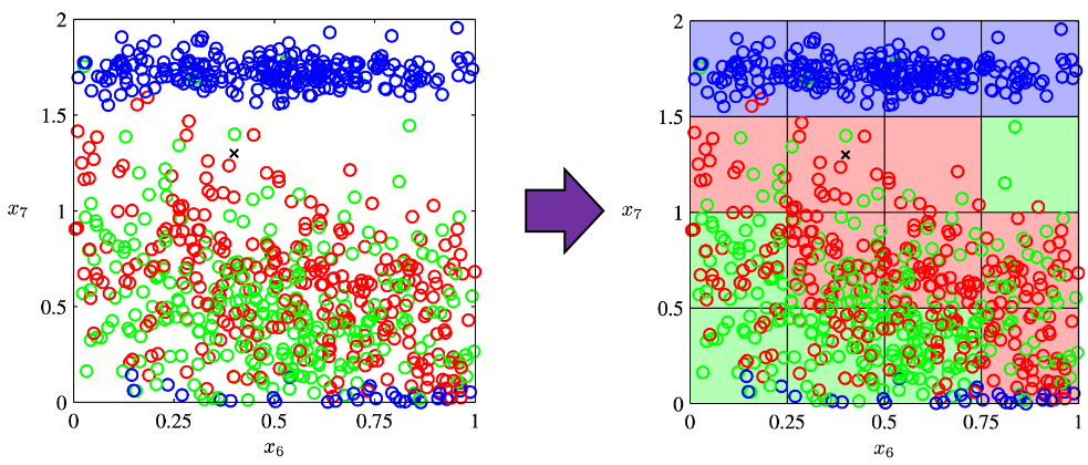
Source: C.M. Bishop, “Pattern Recognition and Machine Learning,” (2006), Springer, pp. 34-35
As I mentioned in the figure above, we used only two features out of 12 features in total. When the total number of data points is fixed and you add remaining ten axes/features one after another, what would happen? Let’s see what “adding axes/features” means. If you are talking about 1, 2, or 3 dimensional grids, you can visualize them. And as you can see from the figure below, if you make each  grids respectively in 1, 2, 3 dimensional spaces, the number of the small regions in the grids are respectively 10, 100, 1000. Even though you cannot visualize it anymore, you can make grids for more than 3 dimensional data. If you continue increasing the degree of dimension, the number of grids increases exponentially, and that can soon surpass the number of training data points. That means there would be a lot of empty spaces in such high dimensional grids. And the classifying method above: coloring each grid and classifying unknown samples depending on the colors of the grids, does not work out anymore because there would be a lot of empty grids.
* If you are still puzzled by the idea of “more than 3 dimensional grids,” you should not think too much about that now. It is enough if you can get some understandings on high dimensional data after reading the whole article of this.
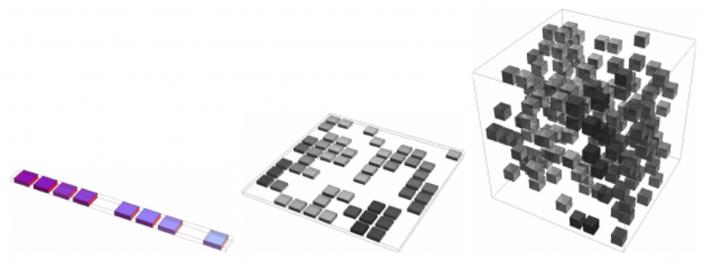
Source: Goodfellow and Yoshua Bengio and Aaron Courville, Deep Learning, (2016), MIT Press, p. 153
I said the method above is the most naive way, but other classical classification methods , for example k-nearest neighbors algorithm, are more or less base on a similar idea. Many of classical machine learning algorithms are based on the idea of smoothness prior, or local constancy prior. In short in classical ways, you do not expect data to change so much in a small region, so you can expect unknown samples to be similar to data in vicinity. But that soon turns out to be problematic when the dimension of data is bigger because training data would be sparse because the area of multidimensional space grows exponentially as I mentioned above. And sometimes you would not be able to find training data around test data. Plus, in high dimensional data, you cannot treat distance in the same as you do in lower dimensional space. The ideas of “close,” “nearby,” or “vicinity” get more obscure in high dimensional data. That point is related to the next topic: the intuition have cultivated in normal life is not applicable to higher dimensional data.
2. Bizarre characteristics of high dimensional data
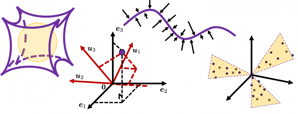
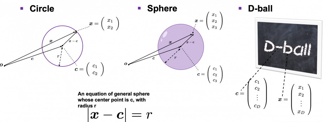
We form our sense of recognition in 3-dimensional ways in our normal life. Even though we can visualize only 1, 2, or 3 dimensional data, we can actually generalize the ideas in 1, 2, or 3 dimensional ideas to higher dimensions. For example 4 dimensional cubes, 100 dimensional spheres, or orthogonality in 255 dimensional space. Again, you cannot exactly visualize those ideas, and for many people, such high dimensional phenomenon are just imaginary matters on blackboards. Those high dimensional ideas are designed to retain some conditions just as well as 1, 2, or 3 dimensional space. Let’s take an example of spheres in several dimensional spaces. General spheres in any D-dimensional space can be defined as a set of any  , such that
  , where
  is the center point and
  is length of radius. When is 2-dimensional, the spheres are called “circles.” When is 3-dimensional, the spheres are called “spheres” in our normal life, unless it is used in a conversation in a college cafeteria, by some students in mathematics department. And when is D-dimensional, they are called D-ball, and again, this is just a imaginary phenomenon on blackboard.
* Vectors and points are almost the same because all the vectors are denoted as “arrows” from the an origin point to sample data points. The only difference is that when you use vectors, you have to consider their directions.
* “D-ball” is usually called “n-ball,” and in such context it is a sphere in a n-dimensional space. But please let me use the term “D-ball” in this article.
Not only spheres, but only many other ideas have been generalized to D-dimensional space, and many of them are indispensable also for data science. But there is one severe problem: the behaviors of data in high dimensional field is quite different from those in two or three dimensional space. To be concrete, in high dimensional field, cubes are spiky, you have to move like Pac-Man, and M & M’s Chocolate looks empty inside but tastes normal.
2.1: spiky cubes
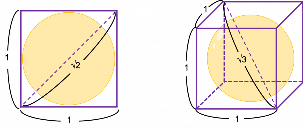
Let’s take a look at an elementary-school-level example of geometry first. Assume that you have several unit squares or unit cubes like below. In each of them a circle or sphere with diameter 1 is inscribed. The length of a diagonal line in each square is  , and that in each cube is
  .
. 
If you stack the squares or cubes as below, what are the length of diameters of the blue circle or sphere, circumscribing all the 4 orange circles or the 8 orange spheres?
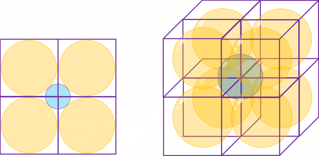
The answers are, the diameter of the blue circle is  , and the diameter of the blue sphere is
  .
.
Next let’s think about the same situation in higher dimensional space. Assume that there are some unit D-dimensional hypercubes stacked, in each of which a D-ball with diameter 1 is inscribed, touching all the surfaces inside. Then what is the length of the diameter of a D-ball circumscribing all the unit D-ball in the hypercubes ? Given the results above, it ca be predicted that its diameter is  . If that is true, there is one strange point:
  can soon surpass 2: that means in the chart above the blue sphere will stick out of the stacked cubes. That sounds like a paradox, but with one hypothesis, the phenomenon makes sense: cubes become more spiky as the degree of dimension grows. This hypothesis is a natural deduction because diagonal lines of hyper cubes get longer, and the the center of each surface of hypercubes still touches the unit D-ball with diameter 1, inscribing inscribing inside each unit hypercube.
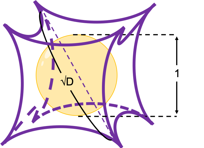
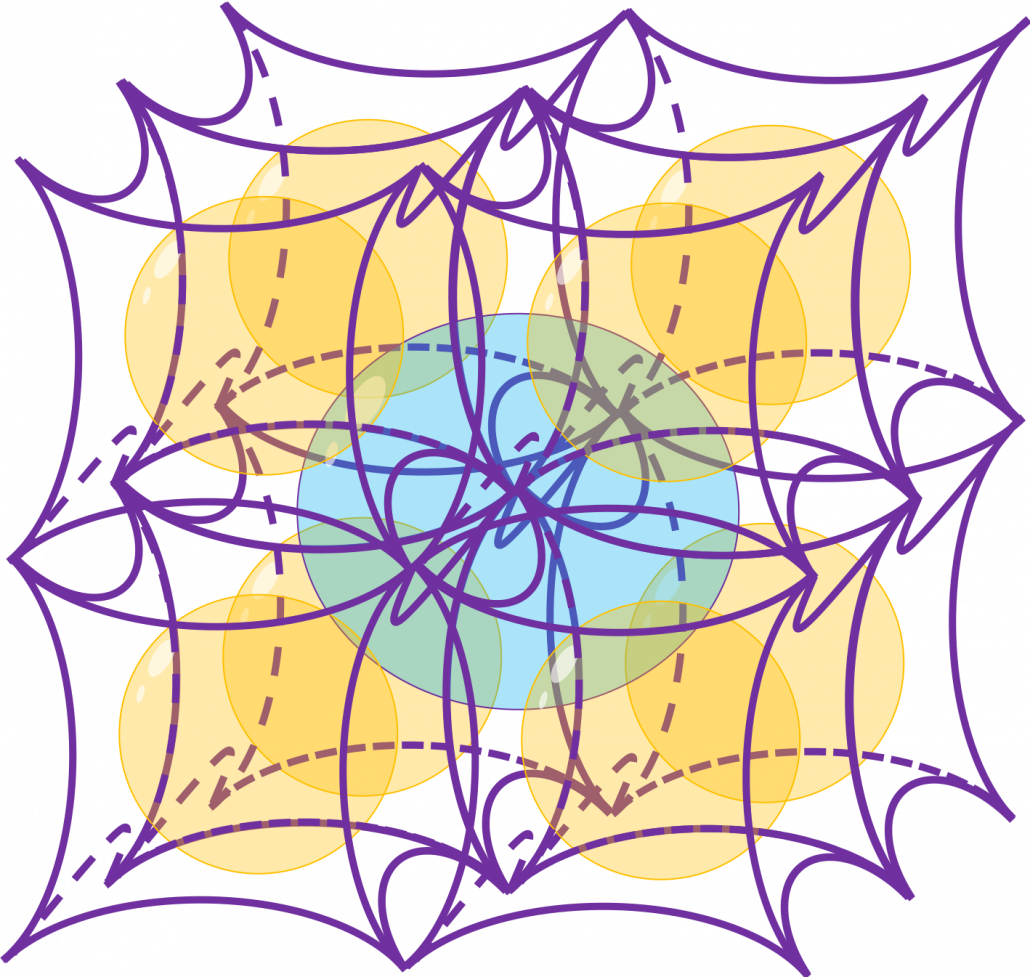
If you stack 4 hypercubes, the blue sphere circumscribing them will not stick out of the stacked hypercubes anymore like the figure below.
*Of course you cannot visualize what is going on in D-dimensional space, so the figure below is just a pseudo simulation of D-dimensional space in our 3-dimensional sense. I guess you have to stack more than four hyper cubes in higher dimensional data, but you cannot easily imagine what will go on in such space anymore.
*You can confirm the fact that hypercube gets more spiky as the degree of dimension growth, by comparing the volume of the hypercube and the volume of the D-ball inscribed inside the hypercube. Thereby you can prove that the volume of hypercube concentrates on the corners of the hypercube. Plus, as I mentioned the longest diagonal distance of hypercube gets longer as dimension degree increases. That is why hypercube is said to be spiky. For mathematical proof, please check the Exercise 1.19 of PRML.
2.2: Pac-Man walking
Next intriguing phenomenon in high dimensional field is that most of pairs of vectors in high dimensional space are orthogonal. In other words, if you select two random vectors in high dimensional space, the angle between them are mostly close to  . Let’s see the general meaning of angle between two vectors in any dimensional spaces. Assume that the angle between two vectors
  , and
, and  is
is  , then
  is calculated as
  . In 1, 2, or 3 dimensional space, you can actually see the angle, but again you can define higher dimensional angle, which you cannot visualize anymore. And angles are sometimes used as similarity of two vectors.
*  is the inner product of , and .
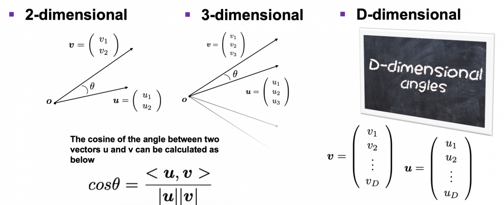
Assume that you generate a pair of two points inside a D-dimensional unit sphere and make two vectors , and by connecting the origin point and those two points respectively. When D is 2, I mean spheres are circles in this case, any are equally generated as in the chart below. The fact might be the same as your intuition. 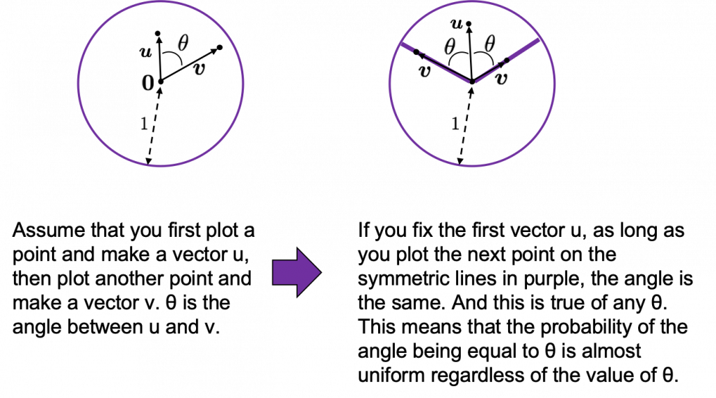 How about in 3-dimensional space? In fact the distribution of is not uniform.
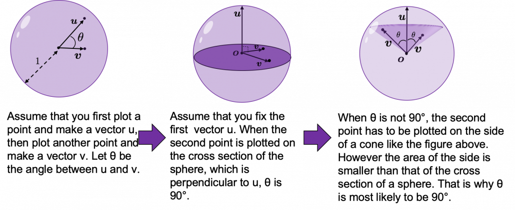
  is the most likely to be generated. As I explain in the figure below, if you compare the area of cross section of a hemisphere and the area of a cone whose vertex is the center point of the sphere, you can see why.
I generated 10000 random pairs of points in side a D-dimensional unit sphere, and calculated the angle between them. In other words I just randomly generated two D-dimensional vectors and , whose elements are randomly generated values between -1 and 1, and calculated the angle between them, repeating this process 10000 times. The chart below are the histograms of angle between pairs of generated vectors in respectively 2, 3, 50, and 100 dimensional space.
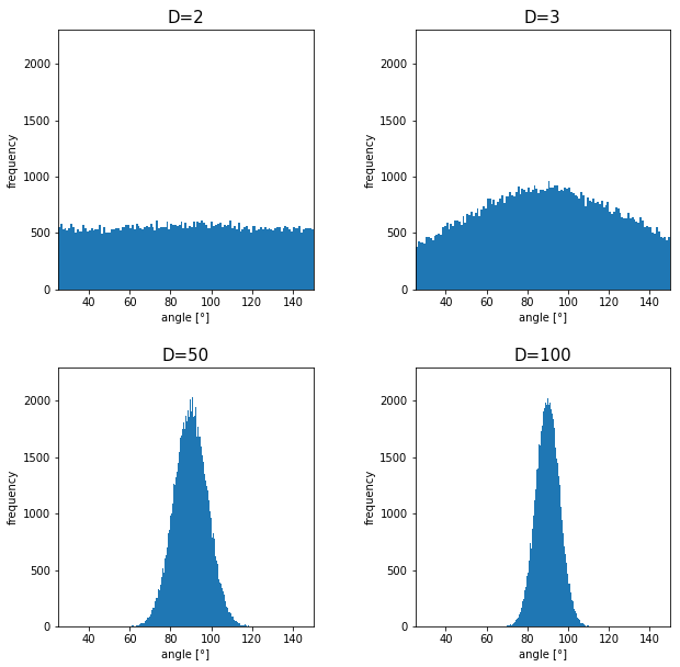
As I explained above, in 2-dimensional space, the distribution of is almost uniform. However the distribution concentrates a little around in 3-dimensional space. You can see that the bigger the degree of dimension is, the more the angles of generated vectors concentrate around . That means most pairs of vectors in high dimensional space are close to orthogonal. Movements are also sequence of vectors, so when most pairs of movement vectors are orthogonal, that means you can only move like Pac-Man in such space.
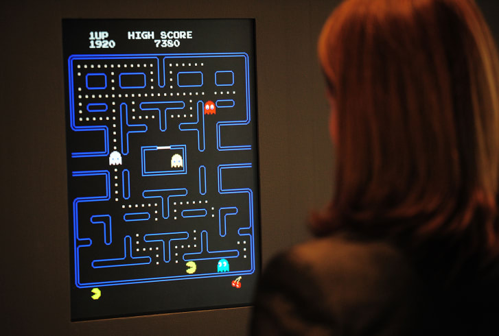
Source: https://edition.cnn.com/style/article/pac-man-40-anniversary-history/index.html
* Of course I am talking about arcade Mac-Man game. Not Pac-Man in Super Smash Bros. Retro RPG video games might have more similar playability, but in high dimensional space it is also difficult to turn back. At any rate, I think you have understood it is even difficult to move smoothly in high dimensional space, just like the first notorious Resident Evil on the first PS console also had terrible playability .
2.3: empty M & M’s chocolate
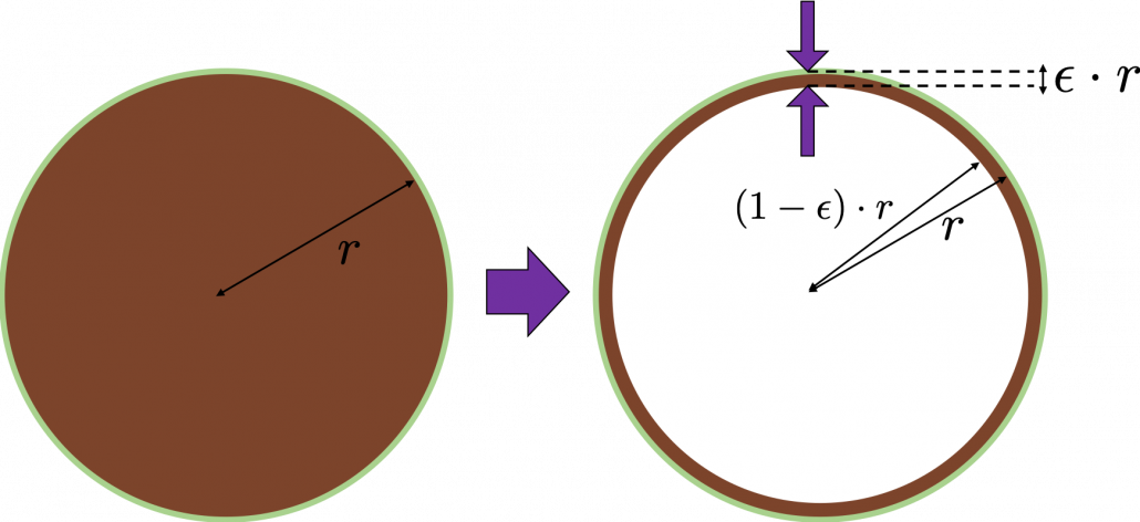
Let’s think about the proportion of the volume of the outermost  surface of general spheres with radius
  First, in 2 two dimensional space, spheres are circles. The area of the brown part of the circle below is
  . In order calculate the are of
  thick surface of the circle, you have only to subtract the area of
  . When
  , the area of outer most surface is
  , and its proportion to the area of the whole circle is
  .
.
In case of 3-dimensional space, the value of a sphere with radius is  , so the proportion of the surface is calculated in the same way:
  . Compared to the case in 2 dimensional space, the proportion is a little bigger.
How about in D-dimensional space? We have seen that even in D-dimensional space the surface of a sphere, I mean D-ball, can be defined as a set of any points whose distance from the center point is all . And it is known that the volume of D-ball is defined as below.

 is called gamma function, but in this article it is not so important. The most important point now is, if you discuss any D-ball, their volume only depends on their radius . That meas the proportion of outer surface of D-ball is calculated as
  . When is 0.01, the proportion of the 1% surface of D-ball changes like in the chart below.
* And of course when  is 2,
is 2,  , and when is 3 ,
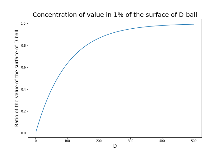
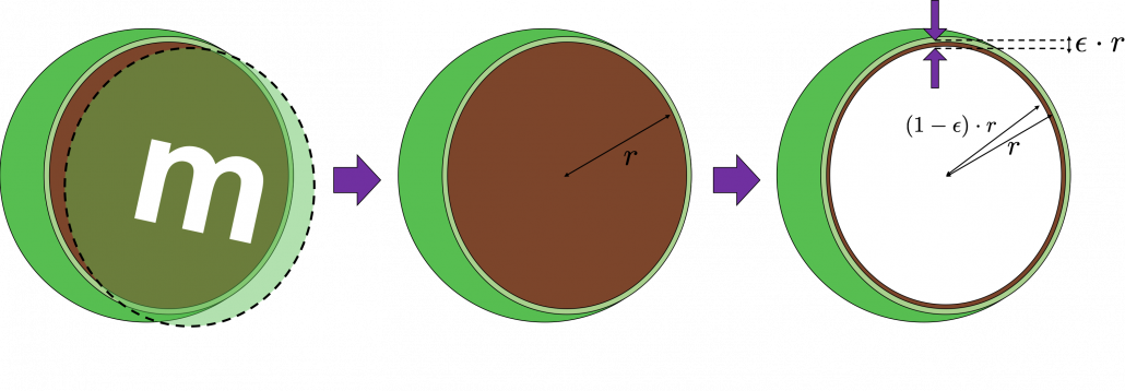
You can see that when D is over 400, around 90% of volume is concentrated in the very thin 1% surface of D-ball. That is why, in high dimensional space, M & M’s chocolate look empty but tastes normal: all the chocolate are concentrated beneath the sugar coating.
More interestingly, even if you choose any points as a central point of a sphere with radius , the other points are squashed to the surface of the sphere, even if all the data points are uniformly distributed. This situation is problematic for classical machine learning algorithms, which are often based on the Euclidean distances between pairs of two sample data points: if you go from the central point to another sample point, the possibility of finding the point within  radius of the center is almost zero. But if you reach the outermost part of the surface of the sphere, most data points are there. However, for one of the data points in the surface, any other data points are distant in the same way.
Inside M & M’s chocolate is a mysterious world.

Source: https://hipwallpaper.com/mms-wallpapers/
You have seen that using high dimensional data can be problematic in many ways. Data science and machine learning are largely based on one idea: you can find a lower dimensional meaningful and easier structure in data. In the next articles I am going to introduce some famous dimension reduction algorithms. And hopefully I would like to give some deeper insights in to these algorithms, in straightforward ways.
* I could not explain the relationships of variance and bias of data. This is also a very important factor when you think about dimensionality of data. I hope I can write about this topic someday. You can also look it up if you are interested.
* I make study materials on machine learning, sponsored by DATANOMIQ. I do my best to make my content as straightforward but as precise as possible. I include all of my reference sources. If you notice any mistakes in my materials, including grammatical errors, please let me know (email: yasuto.tamura@datanomiq.de). And if you have any advice for making my materials more understandable to learners, I would appreciate hearing it.


Leave a Reply
Want to join the discussion?Feel free to contribute!