This is the second article of the series My elaborate study notes on reinforcement learning.
1, Before getting down on business
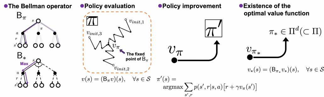
As the title of this article suggests, this article is going to be mainly about the Bellman equation and dynamic programming (DP), which are to be honest very typical and ordinary topics. One typical way of explaining DP in contexts of reinforcement learning (RL) would be explaining the Bellman equation, value iteration, and policy iteration, in this order. If you would like to merely follow pseudocode of them and implement them, to be honest that is not a big deal. However even though I have studied RL only for some weeks, I got a feeling that these algorithms, especially policy iteration are more than just single algorithms. In order not to miss the points of DP, rather than typically explaining value iteration and policy iteration, I would like to take a different approach. Eventually I am going to introduce DP in RL as a combination of the following key terms: the Bellman operator, the fixed point of a policy, policy evaluation, policy improvement, and existence of the optimal policy. But first, in this article I would like to cover basic and typical topics of DP in RL.
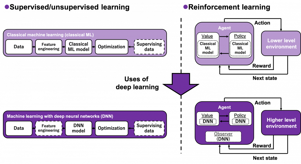
Many machine learning algorithms which use supervised/unsupervised learning more or less share the same ideas. You design a model and a loss function and input samples from data, and you adjust parameters of the model so that the loss function decreases. And you usually use optimization techniques like stochastic gradient descent (SGD) or ones derived from SGD. Actually feature engineering is needed to extract more meaningful information from raw data. Or especially in this third AI boom, the models are getting more and more complex, and I would say the efforts of feature engineering was just replaced by those of designing neural networks. But still, once you have the whole picture of supervised/unsupervised learning, you would soon realize other various algorithms is just a matter of replacing each component of the workflow. However reinforcement learning has been another framework of training machine learning models. Richard E. Bellman’s research on DP in 1950s is said to have laid a foundation for RL. RL also showed great progress thanks to development of deep neural networks (DNN), but still you have to keep it in mind that RL and supervised/unsupervised learning are basically different frameworks. DNN are just introduced in RL frameworks to enable richer expression of each component of RL. And especially when RL is executed in a higher level environment, for example screens of video games or phases of board games, DNN are needed to process each state of the environment. Thus first of all I think it is urgent to see ideas unique to RL in order to effectively learn RL. In the last article I said RL is an algorithm to enable planning by trial and error in an environment, when the model of the environment is not known. And DP is a major way of solving planning problems. But in this article and the next article, I am mainly going to focus on a different aspect of RL: interactions of policies and values.
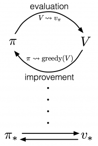 According to a famous Japanese textbook on RL named “Machine Learning Professional Series: Reinforcement Learning,” most study materials on RL lack explanations on mathematical foundations of RL, including the book by Sutton and Barto. That is why many people who have studied machine learning often find it hard to get RL formulations at the beginning. The book also points out that you need to refer to other bulky books on Markov decision process or dynamic programming to really understand the core ideas behind algorithms introduced in RL textbooks. And I got an impression most of study materials on RL get away with the important ideas on DP with only introducing value iteration and policy iteration algorithms. But my opinion is we should pay more attention on policy iteration. And actually important RL algorithms like Q learning, SARSA, or actor critic methods show some analogies to policy iteration. Also the book by Sutton and Barto also briefly mentions “Almost all reinforcement learning methods are well described as GPI (generalized policy iteration). That is, all have identifiable policies and value functions, with the policy always being improved with respect to the value function and the value function always being driven toward the value function for the policy, as suggested by the diagram to the right side.“
Even though I arrogantly, as a beginner in this field, emphasized “simplicity” of RL in the last article, in this article I am conversely going to emphasize the “profoundness” of DP over two articles. But I do not want to cover all the exhaustive mathematical derivations for dynamic programming, which would let many readers feel reluctant to study RL. I tried as hard as possible to visualize the ideas in DP in simple and intuitive ways, as far as I could understand. And as the title of this article series shows, this article is also a study note for me. Any corrections or advice would be appreciated via email or comment pots below.
2, Taking a look at what DP is like
In the last article, I said that planning or RL is a problem of finding an optimal policy  for choosing which actions to take depending on where you are. Also in the last article I displayed flows of blue arrows for navigating a robot as intuitive examples of optimal policies in planning or RL problems. But you cannot directly calculate those policies. Policies have to be evaluated in the long run so that they maximize returns, the sum of upcoming rewards. Then in order to calculate a policy
  , you need to calculate a value functions
  . is a function of how good it is to be in a given state
  , under a policy
  . That means it is likely you get higher return starting from , when is high. As illustrated in the figure below, values and policies, which are two major elements of RL, are updated interactively until they converge to an optimal value or an optimal policy. The optimal policy and the optimal value are denoted as
  and
and  respectively.
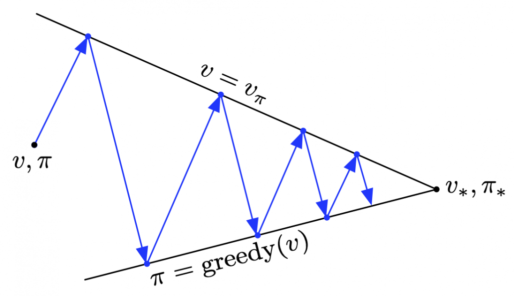
Dynamic programming (DP) is a family of algorithms which is effective for calculating the optimal value and the optimal policy when the complete model of the environment is given. Whether in my articles or not, the rest of discussions on RL are more or less based on DP. RL can be viewed as a method of achieving the same effects as DP when the model of the environment is not known. And I would say the effects of imitating DP are often referred to as trial and errors in many simplified explanations on RL. If you have studied some basics of computer science, I am quite sure you have encountered DP problems. With DP, in many problems on textbooks you find optimal paths of a graph from a start to a goal, through which you can maximizes the sum of scores of edges you pass. You might remember you could solve those problems in recursive ways, but I think many people have just learnt very limited cases of DP. For the time being I would like you to forget such DP you might have learned and comprehend it as something you newly start learning in the context of RL.
*As a more advances application of DP, you might have learned string matching. You can calculated how close two strings of characters are with DP using string matching.
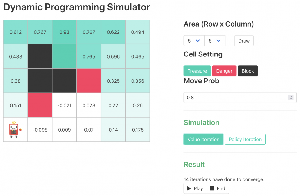
The way of calculating and with DP can be roughly classified to two types, policy-based and value-based. Especially in the contexts of DP, the policy-based one is called policy iteration, and the values-based one is called value iteration. The biggest difference between them is, in short, policy iteration updates a policy every times step, but value iteration does it only at the last time step. I said you alternate between updating and , but in fact that is only true of policy iteration. Value iteration updates a value function  . Before formulating these algorithms, I think it will be effective to take a look at how values and policies are actually updated in a very simple case. I would like to introduce a very good tool for visualizing value/policy iteration. You can customize a grid map and place either of “Treasure,” “Danger,” and “Block.” You can choose probability of transition and either of settings, “Policy Iteration” or “Values Iteration.” Let me take an example of conducting DP on a gird map like below. Whichever of “Policy Iteration” or “Values Iteration” you choose, you would get numbers like below. Each number in each cell is the value of each state, and you can see that when you are on states with high values, you are more likely to reach the “treasure” and avoid “dangers.” But I bet this chart does not make any sense if you have not learned RL yet. I prepared some code for visualizing the process of DP on this simulator. The code is available in this link.
*In the book by Sutton and Barto, when RL/DP is discussed at an implementation level, the estimated values of or  can be denoted as an array
  or
or  . But I would like you take it easy while reading my articles. I will repeatedly mentions differences of notations when that matters.
*Remember that at the beginning of studying RL, only super easy cases are considered, so a is usually just a NumPy array or an Excel sheet.
*The chart above might be also misleading since there is something like a robot at the left bottom corner, which might be an agent. But the agent does not actually move around the environment in planning problems because it has a perfect model of the environment in the head.
The visualization I prepared is based on the implementation of the simulator, so they would give the same outputs. When you run policy iteration in the map, the values and polices are updated as follows. The arrow in each cell is the policy in the state. At each time step the arrows is calculated in a greedy way, and each arrow at each state shows the direction in which the agent is likely to get the highest reward. After 3 iterations, the policies and values converge, and with the policies you can navigate yourself to the “Treasure,” avoiding “Dangers.”
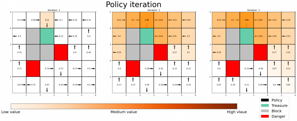
*I am not sure why policies are incorrect at the most left side of the grid map. I might need some modification of code.
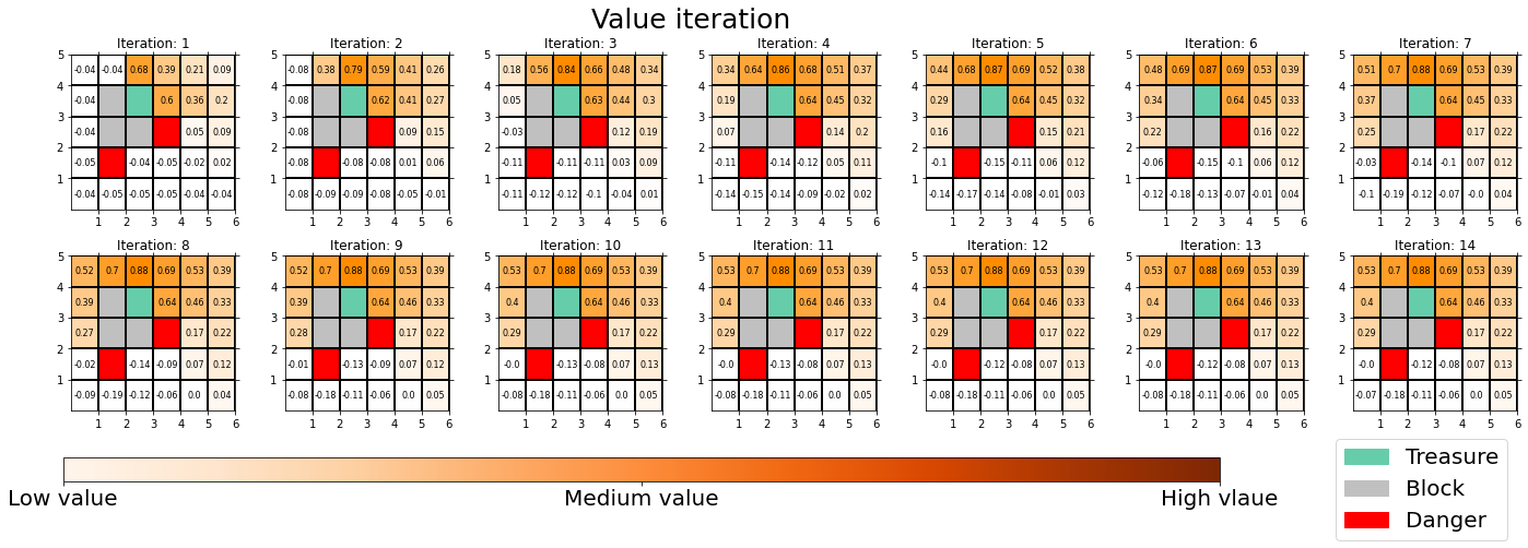
You can also update values without modifying policies as the chart below. In this case only the values of cells are updated. This is value-iteration, and after this iteration converges, if you transit to an adjacent cell with the highest value at each cell, you can also navigate yourself to the “treasure,” avoiding “dangers.”
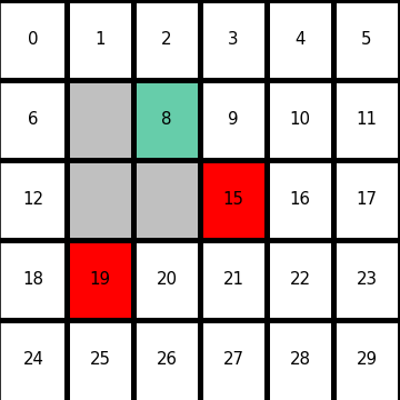
I would like to start formulating DP little by little,based on the notations used in the RL book by Sutton. From now on, I would take an example of the  grid map which I visualized above. In this case each cell is numbered from
  to
to  as the figure below. But the cell 7, 13, 14 are removed from the map. In this case
  , and
, and  . When you pass
  , you get a reward
  , and when you pass the states
  or
or  , you get a reward
  . Also, the agent is encouraged to reach the goal as soon as possible, thus the agent gets a regular reward of
  every time step.
In the last section, I mentioned that the purpose of RL is to find the optimal policy which maximizes a return, the sum of upcoming reward  . A return is calculated as follows.

In RL a return is estimated in probabilistic ways, that is, an expectation of the return given a state  needs to be considered. And this is the value of the state. Thus the value of a state is calculated as follows.
![\mathbb{E}_{\pi}\bigl[R_{t+1} + R_{t+2} + R_{t+3} + \cdots + R_T | S_t = s \bigr]](https://data-science-blog.com/en/wp-content/ql-cache/quicklatex.com-1446ab2bd566ff9ae22a26979bc864a2_l3.png "Rendered by QuickLaTeX.com")
In order to roughly understand how this expectation is calculated let’s take an example of the grid map above. When the current state of an agent is  , it can take numerous patterns of actions. For example (a)
  , (b)
, (b)  , (c)
, (c)  . The rewards after each behavior is calculated as follows.
- If you take a you take the course (a) , you get a reward of
 in total. The probability of taking a course of a) is


- Just like the case of (a), the reward after taking the course
 is
is  . The probability of taking the action can be calculated in the same way as
 .
.
- The rewards and the probability of the case (c) cannot be calculated because future behaviors of the agent is not confirmed.
Assume that (a) and (b) are the only possible cases starting from , under the policy , then the the value of can be calculated as follows as a probabilistic sum of rewards of each behavior (a) and (b).
![\mathbb{E}_{\pi}\bigl[R_{t+1} + R_{t+2} + R_{t+3} + \cdots + R_T | S_t = s \bigr] = r_a \cdot p_a + r_b \cdot p_b](https://data-science-blog.com/en/wp-content/ql-cache/quicklatex.com-9af1a6e1d05f0e084ca3df7b2cab9ef9_l3.png "Rendered by QuickLaTeX.com")
But obviously this is not how values of states are calculated in general. Starting from a state a state , not only (a) and (b), but also numerous other behaviors of agents can be considered. Or rather, it is almost impossible to consider all the combinations of actions, transition, and next states. In practice it is quite difficult to calculate a sequence of upcoming rewards  ,and it is virtually equal to considering all the possible future cases.A very important formula named the Bellman equation effectively formulate that.
3, The Bellman equation and convergence of value functions
The Bellman equation enables estimating values of states considering future countless possibilities with the following two ideas.
- Returns are calculated recursively.
- Returns are calculated in probabilistic ways.
First of all, I have to emphasize that a discounted return is usually used rather than a normal return, and a discounted one is defined as below

, where ![\gamma \in (0, 1]](https://data-science-blog.com/en/wp-content/ql-cache/quicklatex.com-914da56af30aaafcc35b558976e8fdca_l3.png "Rendered by QuickLaTeX.com") is a discount rate. (1)As the first point above, the discounted return can be calculated recursively as follows:
is a discount rate. (1)As the first point above, the discounted return can be calculated recursively as follows: 

 . You can postpone calculation of future rewards corresponding to
  this way. This might sound obvious, but this small trick is crucial for defining defining value functions or making update rules of them. (2)The second point might be confusing to some people, but it is the most important in this section. We took a look at a very simplified case of calculating the expectation in the last section, but let’s see how a value function is defined in the first place.
![v_{\pi}(s) \doteq \mathbb{E}_{\pi}\bigl[G_t | S_t = s \bigr]](https://data-science-blog.com/en/wp-content/ql-cache/quicklatex.com-4a07b7408b4cebfe6e2558ca8d1573cf_l3.png "Rendered by QuickLaTeX.com")
This equation means that the value of a state is a probabilistic sum of all possible rewards taken in the future following a policy . That is, is an expectation of the return, starting from the state . The definition of a values is written down as follows, and this is what  means.
![v_{\pi} (s)= \sum_{a}{\pi(a|s) \sum_{s', r}{p(s', r|s, a)\bigl[r + \gamma v_{\pi}(s')\bigr]}}](https://data-science-blog.com/en/wp-content/ql-cache/quicklatex.com-9b05fc8f5122733b29e251f8000f7bf2_l3.png "Rendered by QuickLaTeX.com")
This is called Bellman equation, and it is no exaggeration to say this is the foundation of many of upcoming DP or RL ideas. Bellman equation can be also written as ![\sum_{s', r, a}{\pi(a|s) p(s', r|s, a)\bigl[r + \gamma v_{\pi}(s')\bigr]}](https://data-science-blog.com/en/wp-content/ql-cache/quicklatex.com-c9afc3114f14adcf06a184c6656f404b_l3.png "Rendered by QuickLaTeX.com") . It can be comprehended this way: in Bellman equation you calculate a probabilistic sum of
. It can be comprehended this way: in Bellman equation you calculate a probabilistic sum of  , considering all the possible actions of the agent in the time step. is a sum of the values of the next state
  and a reward
  , which you get when you transit to the state from . The probability of getting a reward after moving from the state to , taking an action
  is
is  . Hence the right side of Bellman equation above means the sum of
 ![\pi(a|s) p(s', r|s, a)\bigl[r + \gamma v_{\pi}(s')\bigr]](https://data-science-blog.com/en/wp-content/ql-cache/quicklatex.com-c68792d33ebf817bf92b2c3122432011_l3.png "Rendered by QuickLaTeX.com") , over all possible combinations of , , and .
, over all possible combinations of , , and .
*I would not say this equation is obvious, and please let me explain a proof of this equation later.
The following figures are based on backup diagrams introduced in the book by Sutton and Barto. As we have just seen, Bellman expectation equation calculates a probabilistic summation of  . In order to calculate the expectation, you have to consider all the combinations of , , and . The backup diagram at the left side below shows the idea as a decision-tree-like graph, and strength of color of each arrow is the probability of taking the path.
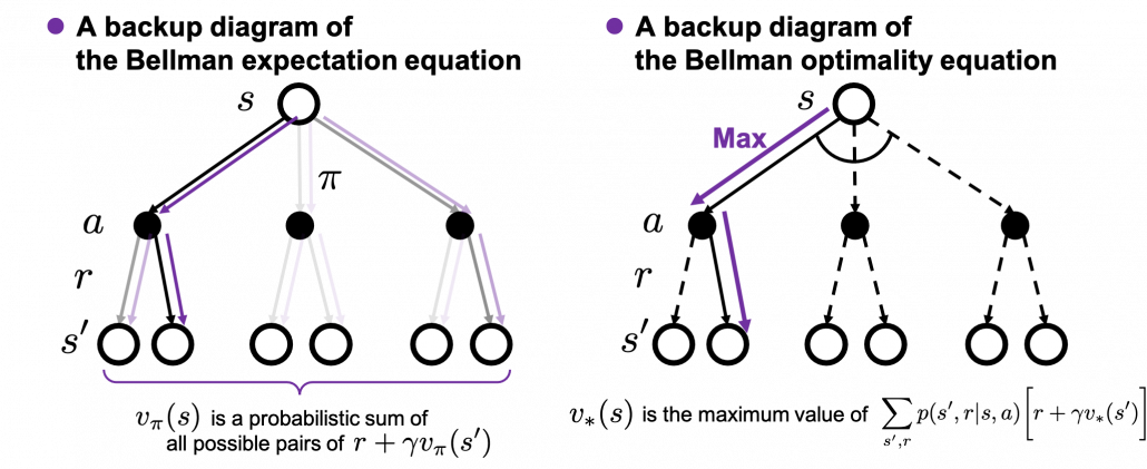
The Bellman equation I have just introduced is called Bellman expectation equation to be exact. Like the backup diagram at the right side, there is another type of Bellman equation where you consider only the most possible path. Bellman optimality equation is defined as follows.
![v_{\ast}(s) \doteq \max_{a} \sum_{s', r}{p(s', r|s, a)\bigl[r + \gamma v_{\ast}(s')\bigr]}](https://data-science-blog.com/en/wp-content/ql-cache/quicklatex.com-86f7734f497416e3b1922ee15d1688dc_l3.png "Rendered by QuickLaTeX.com")
I would like you to pay attention again to the fact that in definitions of Bellman expectation/optimality equations, / is defined recursively with /. You might have thought how to calculate / is the problem in the first place.
As I implied in the first section of this article, ideas behind how to calculate these and should be discussed more precisely. Especially how to calculate is a well discussed topic in RL, including the cases where data is sampled from an unknown environment model. In this article we are discussing planning problems, where a model an environment is known. In planning problems, that is DP problems where all the probabilities of transition  are known, a major way of calculating is iterative policy evaluation. With iterative policy evaluation a sequence of value functions
  converges to with the following recurrence relation
![v_{k+1}(s) =\sum_{a}{\pi(a|s)\sum_{s', r}{p(s', r | s, a) [r + \gamma v_k (s')]}}](https://data-science-blog.com/en/wp-content/ql-cache/quicklatex.com-0d6a73bc17d541f77b43a10e128462ce_l3.png "Rendered by QuickLaTeX.com") .
.
Once  converges to , finally the equation of the definition of holds as follows.
![v_{\pi}(s) =\sum_{a}{\pi(a|s)\sum_{s', r}{p(s', r | s, a) [r + \gamma v_{\pi} (s')]}}](https://data-science-blog.com/en/wp-content/ql-cache/quicklatex.com-afdb0cd8be05e7e79fc3306f8ebc3732_l3.png "Rendered by QuickLaTeX.com") .
.
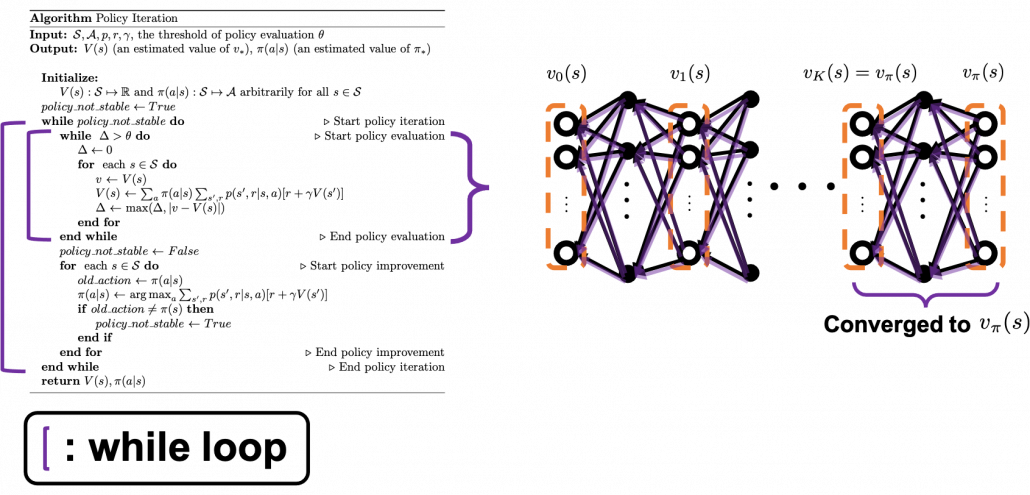
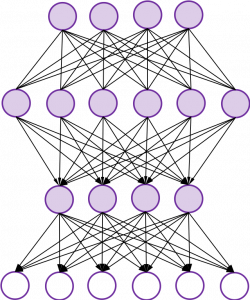
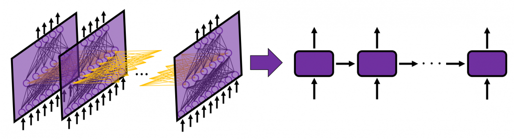
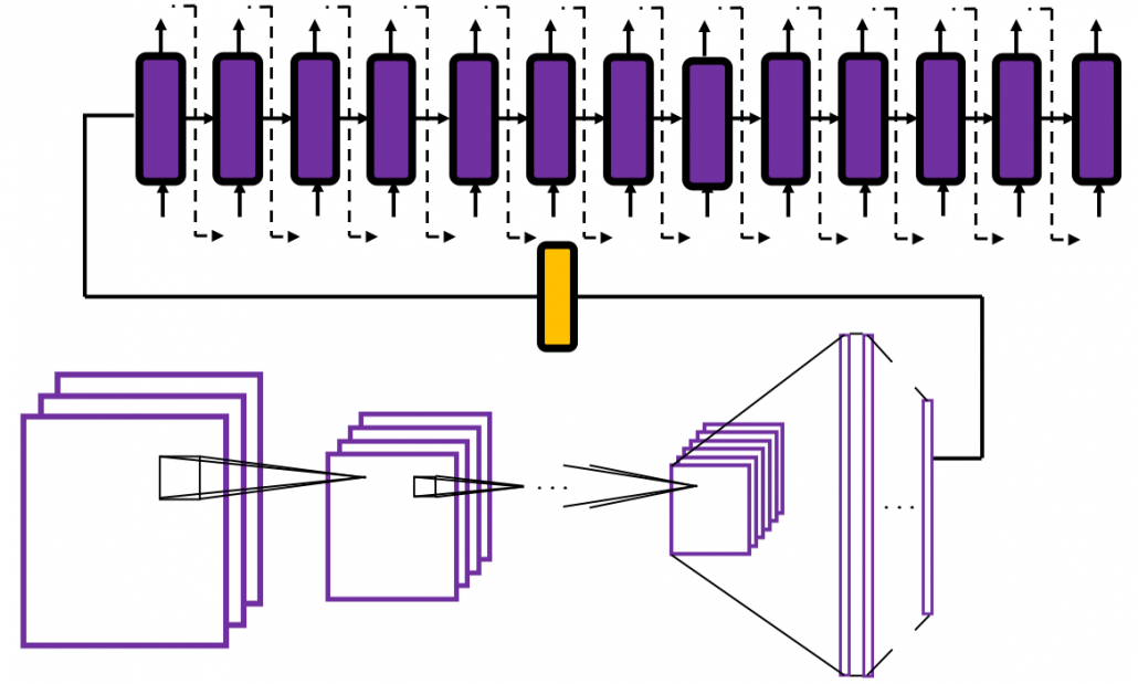
The convergence to is like the graph below. If you already know how to calculate forward propagation of a neural network, this should not be that hard to understand. You just expand recurrent relation of and  from the initial value at
  to the converged state at
  . But you have to be careful abut the directions of the arrows in purple. If you correspond the backup diagrams of the Bellman equation with the graphs below, the purple arrows point to the reverse side to the direction where the graphs extend. This process of converging an arbitrarily initialized
  to is called policy evaluation.
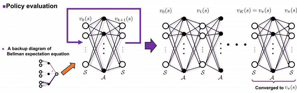
* are a set of states and actions respectively. Thus
  , the size of
  is the number of white nodes in each layer, and the number of black nodes.
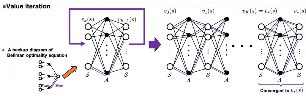
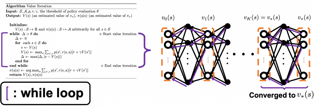
The same is true of the process of calculating an optimal value function . With the following recurrence relation
![v_{k+1}(s) =\max_a\sum_{s', r}{p(s', r | s, a) [r + \gamma v_k (s')]}](https://data-science-blog.com/en/wp-content/ql-cache/quicklatex.com-798ecf9bb29b6fcdecb3282f759d07d2_l3.png "Rendered by QuickLaTeX.com")
converges to an optimal value function . The graph below visualized the idea of convergence.
4, Pseudocode of policy iteration and value iteration
I prepared pseudocode of each algorithm based on the book by Sutton and Barto. These would be one the most typical DP algorithms you would encounter while studying RL, and if you just want to implement RL by yourself, these pseudocode would enough. Or rather these would be preferable to other more general and abstract pseudocode. But I would like to avoid explaining these pseudocode precisely because I think we need to be more conscious about more general ideas behind DP, which I am going to explain in the next article. I will cover only the important points of these pseudocode, and I would like to introduce some implementation of the algorithms in the latter part of next article. I think you should briefly read this section and come back to this section section or other study materials after reading the next article. In case you want to check the algorithms precisely, you could check the pseudocode I made with LaTeX in this link.
The biggest difference of policy iteration and value iteration is the timings of updating a policy. In policy iteration, a value function and are arbitrarily initialized. (1)The first process is policy evaluation. The policy is fixed, and the value function approximately converge to , which is a value function on the policy . This is conducted by the iterative calculation with the reccurence relation introduced in the last section.(2) The second process is policy improvement. Based on the calculated value function , the new policy is updated as below.
![\pi(a|s) \gets\text{argmax}_a {r + \sum_{s', r}{p(s', r|s, a)[r + \gamma V(s')]}}, \quad \forall s\in \mathcal{S}](https://data-science-blog.com/en/wp-content/ql-cache/quicklatex.com-5f4b9305832f16e171d2d5428f5251d8_l3.png "Rendered by QuickLaTeX.com")
The meaning of this update rule of a policy is quite simple: is updated in a greedy way with an action such that ![r + \sum_{s', r}{p(s', r|s, a)[r + \gamma V(s')]}](https://data-science-blog.com/en/wp-content/ql-cache/quicklatex.com-3cb4dfa2cd76474740b41aecacce9d84_l3.png "Rendered by QuickLaTeX.com") is maximized. And when the policy is not updated anymore, the policy has converged to the optimal one. At least I would like you to keep it in mind that a while loop of itrative calculation of is nested in another while loop. The outer loop continues till the policy is not updated anymore.
is maximized. And when the policy is not updated anymore, the policy has converged to the optimal one. At least I would like you to keep it in mind that a while loop of itrative calculation of is nested in another while loop. The outer loop continues till the policy is not updated anymore.
On the other hand in value iteration, there is mainly only one loop of updating , which converge to . And the output policy is the calculated the same way as policy iteration with the estimated optimal value function. According to the book by Sutton and Barto, value iteration can be comprehended this way: the loop of value iteration is truncated with only one iteration, and also policy improvement is done only once at the end.
As I repeated, I think policy iteration is more than just a single algorithm. And relations of values and policies should be discussed carefully rather than just following pseudocode. And whatever RL algorithms you learn, I think more or less you find some similarities to policy iteration. Thus in the next article, I would like to introduce policy iteration in more abstract ways. And I am going to take a rough look at various major RL algorithms with the keywords of “values” and “policies” in the next article.
Appendix
I mentioned the Bellman equation is nothing obvious. In this section, I am going to introduce a mathematical derivation, which I think is the most straightforward. If you are allergic to mathematics, the part blow is not recommendable, but the Bellman equation is the core of RL. I would not say this is difficult, and if you are going to read some texts on RL including some equations, I think mastering the operations I explain below is almost mandatory.
First of all, let’s organize some important points. But please tolerate inaccuracy of mathematical notations here. I am going to follow notations in the book by Sutton and Barto.
- Capital letters usually denote random variables. For example
 . And corresponding small letters are realized values of the random variables. For example
  . (*Please do not think too much about the number of
  s on the small letters.)
- Conditional probabilities in general are denoted as for example
 . This means the probability of
  are sampled given that
  is sampled.
- In the book by Sutton and Barto, a probilistic funciton
 means a probability of transition, but I am using to denote probabilities in general. Thus
  shows the probability that, given an agent being in state at time
  , the agent will do action , AND doing this action will cause the agent to proceed to state at time
  , and receive reward . is not defined in the book by Barto and Sutton.
- The following equation holds about any conditional probabilities:
 . Thus importantly,
- When random variables
 are discrete random variables, a conditional expectation of
  given
given  is calculated as follows:
 ![\mathbb{E}[X|Y=y] = \sum_{x}{p(x|Y=y)}](https://data-science-blog.com/en/wp-content/ql-cache/quicklatex.com-5bee0d95ebfa141ff0bc520462f4cfa9_l3.png "Rendered by QuickLaTeX.com") .
.
Keeping the points above in mind, let’s get down on business. First, according to definition of a value function on a policy  and linearity of an expectation, the following equations hold.
![v_{\pi}(s) = \mathbb{E} [G_t | S_t =s] = \mathbb{E} [R_{t+1} + \gamma G_{t+1} | S_t =s]](https://data-science-blog.com/en/wp-content/ql-cache/quicklatex.com-fbb4801687a26cb911e5675ac25002bd_l3.png "Rendered by QuickLaTeX.com")
![=\mathbb{E} [R_{t+1} | S_t =s] + \gamma \mathbb{E} [G_{t+1} | S_t =s]](https://data-science-blog.com/en/wp-content/ql-cache/quicklatex.com-f485080bf287c6c9156187adc49b1b4c_l3.png "Rendered by QuickLaTeX.com")
Thus we need to calculate ![\mathbb{E} [R_{t+1} | S_t =s]](https://data-science-blog.com/en/wp-content/ql-cache/quicklatex.com-a585f119409ea2b556c68a0c1378a356_l3.png "Rendered by QuickLaTeX.com") and
and ![\mathbb{E} [G_{t+1} | S_t =s]](https://data-science-blog.com/en/wp-content/ql-cache/quicklatex.com-7f1e5cf67a9196db4f0aace79e81e322_l3.png "Rendered by QuickLaTeX.com") . As I have explained is the sum of
. As I have explained is the sum of  over all the combinations of
  . And according to one of the points above,
  . Thus the following equation holds.
![\mathbb{E} [R_{t+1} | S_t =s] = \sum_{s', a, r}{p(s', a, r|s)r} =](https://data-science-blog.com/en/wp-content/ql-cache/quicklatex.com-dd202255b6a36417c897509dc2b69655_l3.png "Rendered by QuickLaTeX.com")
 .
.
Next we have to calculate
![\mathbb{E} [G_{t+1} | S_t =s]](https://data-science-blog.com/en/wp-content/ql-cache/quicklatex.com-6bc115f9e71f2fc3a69465acf6a91464_l3.png "Rendered by QuickLaTeX.com")
![= \mathbb{E} [R_{t + 2} + \gamma R_{t + 3} + \gamma ^2 R_{t + 4} + \cdots | S_t =s]](https://data-science-blog.com/en/wp-content/ql-cache/quicklatex.com-48b09c6d0d7d67902de3191e66a38be2_l3.png "Rendered by QuickLaTeX.com")
![= \mathbb{E} [R_{t + 2} | S_t =s] + \gamma \mathbb{E} [R_{t + 2} | S_t =s] + \gamma ^2\mathbb{E} [ R_{t + 4} | S_t =s] +\cdots](https://data-science-blog.com/en/wp-content/ql-cache/quicklatex.com-5cdf22993b5055312df2e1f797fd3b26_l3.png "Rendered by QuickLaTeX.com") .
.
Let’s first calculate ![\mathbb{E} [R_{t + 2} | S_t =s]](https://data-science-blog.com/en/wp-content/ql-cache/quicklatex.com-469530b7d89bba0e743a0a3b1015ccd3_l3.png "Rendered by QuickLaTeX.com") . Also
. Also ![\mathbb{E} [R_{t + 3} | S_t =s]](https://data-science-blog.com/en/wp-content/ql-cache/quicklatex.com-2bb7f6a67696da895bb485861837f1d2_l3.png "Rendered by QuickLaTeX.com") is a sum of
is a sum of  over all the combinations of (s”, a’, r’, s’, a, r).
![\mathbb{E}_{\pi} [R_{t + 2} | S_t =s] =\sum_{s'', a', r', s', a, r}{p(s'', a', r', s', a, r|s)r'}](https://data-science-blog.com/en/wp-content/ql-cache/quicklatex.com-616b7769fe43ea42b46e5ca3f604ccee_l3.png "Rendered by QuickLaTeX.com")


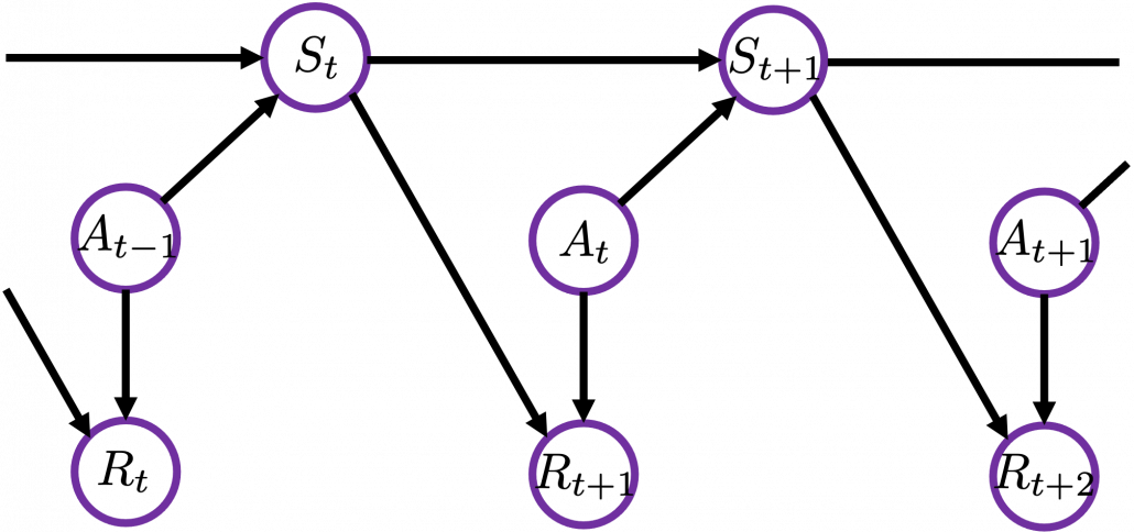
I would like you to remember that in Markov decision process the next state  and the reward only depends on the current state
  and the action
  at the time step.
Thus in variables  , only have the following variables
  . And again
  . Thus the following equations hold.
![\mathbb{E}_{\pi} [R_{t + 2} | S_t =s]=\sum_{ s', a, r}{p(s', a, r|s)} \sum_{s'', a', r'}{p(s'', a', r'| s', a, r', s)r'}](https://data-science-blog.com/en/wp-content/ql-cache/quicklatex.com-1e4e2cb83f6dd183dce4e2a51990bbc2_l3.png "Rendered by QuickLaTeX.com")

![= \sum_{ s', a, r}{p(s', r|a, s)\pi(a|s)} \mathbb{E}_{\pi} [R_{t+2} | s']](https://data-science-blog.com/en/wp-content/ql-cache/quicklatex.com-664e5538f363a0ef817dd5f48fbbae6a_l3.png "Rendered by QuickLaTeX.com") .
.
![\mathbb{E}_{\pi} [R_{t + 3} | S_t =s]](https://data-science-blog.com/en/wp-content/ql-cache/quicklatex.com-64827bc08e99d614dc3838a85798c7d8_l3.png "Rendered by QuickLaTeX.com") can be calculated the same way.
can be calculated the same way.
![\mathbb{E}_{\pi}[R_{t + 3} | S_t =s] =\sum_{s''', a'', r'', s'', a', r', s', a, r}{p(s''', a'', r'', s'', a', r', s', a, r|s)r''}](https://data-science-blog.com/en/wp-content/ql-cache/quicklatex.com-421e1a0b214d777abba77463656339f8_l3.png "Rendered by QuickLaTeX.com")


![=\sum_{ s', a, r}{ p(s', r | s, a)p(a|s)} \mathbb{E}_{\pi} [R_{t+3} | s']](https://data-science-blog.com/en/wp-content/ql-cache/quicklatex.com-6e0ec2657d6aca22c01de6f4b10a136a_l3.png "Rendered by QuickLaTeX.com") .
.
The same is true of calculating ![\mathbb{E}_{\pi} [R_{t + 4} | S_t =s]](https://data-science-blog.com/en/wp-content/ql-cache/quicklatex.com-5370726e4df48fa2beda19166dc02906_l3.png "Rendered by QuickLaTeX.com") ,
, ![\mathbb{E}_{\pi} [R_{t + 5} | S_t =s]\dots](https://data-science-blog.com/en/wp-content/ql-cache/quicklatex.com-c60185b7e16dd3c9d80041a6d63e4901_l3.png "Rendered by QuickLaTeX.com") . Thus
. Thus
![v_{\pi}(s) =\mathbb{E} [R_{t+1} | S_t =s] + \gamma \mathbb{E} [G_{t+1} | S_t =s]](https://data-science-blog.com/en/wp-content/ql-cache/quicklatex.com-e78cd95d37820f82e6dce3d5c5943815_l3.png "Rendered by QuickLaTeX.com")
= ![+ \mathbb{E} [R_{t + 2} | S_t =s] + \gamma \mathbb{E} [R_{t + 3} | S_t =s] + \gamma ^2\mathbb{E} [ R_{t + 4} | S_t =s] +\cdots](https://data-science-blog.com/en/wp-content/ql-cache/quicklatex.com-9d5855daab70bbee7810386c6fc52bc1_l3.png "Rendered by QuickLaTeX.com")

![+\sum_{ s', a, r}{p(s', r|a, s)\pi(a|s)} \mathbb{E}_{\pi} [R_{t+2} |S_{t+1}= s']](https://data-science-blog.com/en/wp-content/ql-cache/quicklatex.com-028766cd22f5479faa5a4f1ea907da6b_l3.png "Rendered by QuickLaTeX.com")
![+\gamma \sum_{ s', a, r}{ p(s', r | s, a)p(a|s)} \mathbb{E}_{\pi} [R_{t+3} |S_{t+1} = s']](https://data-science-blog.com/en/wp-content/ql-cache/quicklatex.com-6679a24522d25f8e36d5caf2a7a8ce06_l3.png "Rendered by QuickLaTeX.com")
![+\gamma^2 \sum_{ s', a, r}{ p(s', r | s, a)p(a|s)} \mathbb{E}_{\pi} [ R_{t+4}|S_{t+1} = s'] + \cdots](https://data-science-blog.com/en/wp-content/ql-cache/quicklatex.com-cb1b0cd6d79e351b146b9b5766c7f5e2_l3.png "Rendered by QuickLaTeX.com")
![=\sum_{ s', a, r}{ p(s', r | s, a)p(a|s)} [r + \mathbb{E}_{\pi} [\gamma R_{t+2}+ \gamma R_{t+3}+\gamma^2R_{t+4} + \cdots |S_{t+1} = s'] ]](https://data-science-blog.com/en/wp-content/ql-cache/quicklatex.com-641a5ebcd67a76dc3f5367ee009e9b14_l3.png "Rendered by QuickLaTeX.com")
![=\sum_{ s', a, r}{ p(s', r | s, a)p(a|s)} [r + \mathbb{E}_{\pi} [G_{t+1} |S_{t+1} = s'] ]](https://data-science-blog.com/en/wp-content/ql-cache/quicklatex.com-133e0a40144cd6b8d9d24eb9c62541a3_l3.png "Rendered by QuickLaTeX.com")
![=\sum_{ s', a, r}{ p(s', r | s, a)p(a|s)} [r + v_{\pi}(s') ]](https://data-science-blog.com/en/wp-content/ql-cache/quicklatex.com-942d98bd0c9d7cc3ed2939137e05df53_l3.png "Rendered by QuickLaTeX.com")


 The most remarkable invention in this time was of course perceptron by Frank Rosenblatt. Some people say that this is the first neural network. Even though you can implement perceptron with a-few-line codes in Python, obviously they did not have Jupyter Notebook in those days. The perceptron was implemented as a huge instrument named Mark 1 Perceptron, and it was composed of randomly connected wires. I do not precisely know how it works, but it was a huge effort to implement even the most primitive type of neural networks. They needed to use a big lighting fixture to get a 20*20 pixel image using 20*20 array of cadmium sulphide photocells. The research by Rosenblatt, however, was criticized by Marvin Minsky in his book because perceptrons could only be used for linearly separable data. To make matters worse the criticism prevailed as that more general, multi-layer perceptrons were also not useful for linearly inseparable data (as I mentioned in the first article, multi-layer perceptrons, namely normal neural networks, can be universal approximators, which have potentials to classify/regress various types of complex data). In case you do not know what “linearly separable” means, imagine that there are data plotted on a piece of paper. If an elementary school kid can draw a border line between two clusters of the data with a ruler and a pencil on the paper, the 2d data is “linearly separable”….
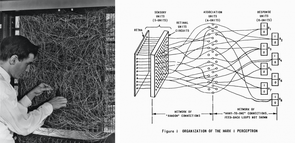


 , which most people would have seen in compulsory education, is a part of mapping. If you get a value x, you get a value y corresponding to the x.
 . If you have never studied linear algebra , imagine that a vector is a column of Excel data (only one column), a matrix is a sheet of Excel data (with some rows and columns), and a tensor is some sheets of Excel data (each sheet does not necessarily contain only one column.)
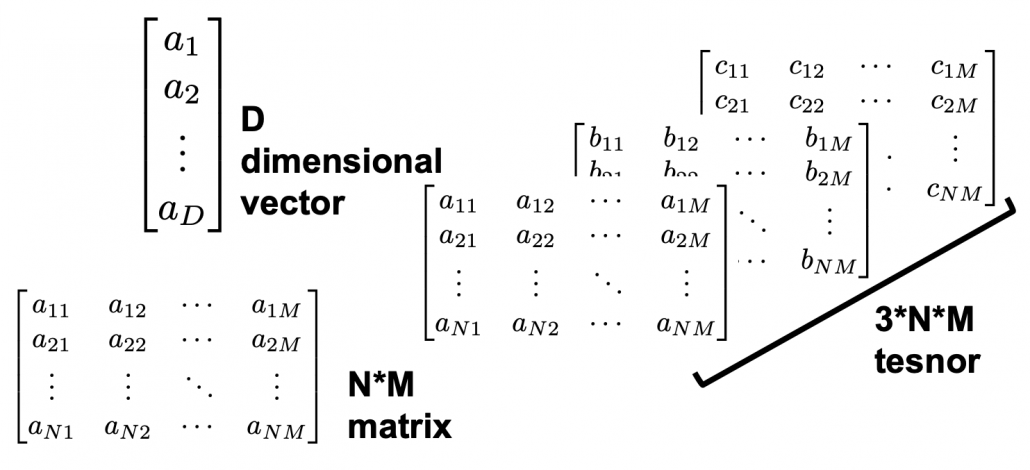


 Ronny Fehling is Partner and Associate Director for Artificial Intelligence as the Boston Consulting Group GAMMA. With more than 20 years of continually progressive experience in leading business and technology innovation, spearheading digital transformation, and aligning the corporate strategy with Artificial Intelligence he industry-leading organizations to grow their top-line and kick-start their digital transformation.