Hand Written Alphabet recognition Using Support Vector Machine

We have used image classification as an task in many cases, more often this has been done using an module like openCV in python or using pre-trained models like in case of MNIST data sets. The idea of using Support Vector Machines for carrying out the same task is to give a simpler approach for a complicated process. There are some pro’s and con’s in every algorithm. Support vector machine for data with very high dimension may prove counter productive. But in case of image data we are actually using a array. If its a mono chrome then its just a 2 dimensional array, if grey scale or color image stack then we may have a 3 dimensional array processing to be considered. You can get more clarity on the array part if you go through this article on Machine learning using only numpy array. While there are certainly advantages of using OCR packages like Tesseract or OpenCV or GPTs, I am putting forth this approach of using a simple SVM model for hand written text classification. As a student while doing linear regression, I learn’t a principle “Occam’s Razor”, Basically means, keep things simple if they can explain what you want to. In short, the law of parsimony, simplify and not complicate. Applying the same principle on Hand written Alphabet recognition is an attempt to simplify using a classic algorithm, the Support Vector Machine. We break the  problem of hand written alphabet recognition into a simple process rather avoiding usage of heavy packages. This is an attempt to create the data and then build a model using Support Vector Machines for Classification.

Data Preparation

Manually edit the data instead of downloading it from the web. This will help you understand your data from the beginning. Manually write some letters on white paper and get the photo from your mobile phone. Then store it on your hard drive. As we are doing a trial we don’t want to waste a lot of time in data creation at this stage, so it’s a good idea to create two or three different characters for your dry run. You may need to change the code as you add more instances of classes, but this is where the learning phase begins. We are now at the training level.

Data Structure

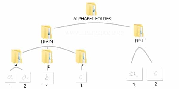
You can create the data yourself by taking standard pictures of hand written text in a 200 x 200 pixel dimension. Alternatively you can use a pen tab to manually write these alphabets and save them as files. If you know and photo editing tools you can use them as well. For ease of use, I have already created a sample data and saved it in the structure as below.

Image Source : From Author

You can download the data which I have used, right click on this download data link and open in new tab or window. Then unzip the folders and you should be able to see the same structure and data as above in your downloads folder. I would suggest, you should create your own data and repeat the  process. This would help you understand the complete flow.

Install the Dependency Packages for RStudio

We will be using the jpeg package in R for Image handling and the SVM implementation from the kernlab package.  Also we need to make sure that the image data has dimension’s of 200 x 200 pixels, with a horizontal and vertical resolution of 120dpi. You can vary the dimension’s like move it to 300 x 300 or reduce it to 100 x 100. The higher the dimension, you will need more compute power. Experiment around the color channels and resolution later once you have implemented it in the current form.

# install package "jpeg"

  install.packages("jpeg", dependencies = TRUE)

# install the "kernlab" package for building the model using support vector machines

install.packages("kernlab", dependencies  = TRUE)

Load the training data set

# load the "jpeg" package for reading the JPEG format files
library(jpeg)

# set the working directory for reading the training image data set
setwd("C:/Users/mohan/Desktop/alphabet_folder/Train")

# extract the directory names for using as image labels

f_train<-list.files()
 

# Create an empty data frame to store the image data labels and the extracted new features in training environment

df_train<- data.frame(matrix(nrow=0,ncol=5))

Feature Transformation

Since we don’t intend to use the typical CNN, we are going to use the white, grey and black pixel values for new feature creation. We will use the summation of all the pixel values of a image  and save it as a new feature called as “sum”, the count of all pixels adding up to zero as “zero”, the count of all pixels adding up to “ones” and the sum of all pixels between zero’s and one’s as “in_between”. The “label” feature names are extracted from the names of the folder

# names the columns of the data frame as per the feature name schema

names(df_train)<- c("sum","zero","one","in_between","label")

# loop to compute as per the logic

counter<-1 

for(i in 1:length(f_train))

{

setwd(paste("C:/Users/mohan/Desktop/alphabet_folder/Train/",f_train[i],sep=""))

 

data_list<-list.files()

 

  for(j in 1:length(data_list))

  {

    temp<- readJPEG(data_list[j])

    df_train[counter,1]<- sum(temp)

    df_train[counter,2]<- sum(temp==0)

    df_train[counter,3]<- sum(temp==1)

    df_train[counter,4]<- sum(temp > 0 & temp < 1)

    df_train[counter,5]<- f_train[i]

    counter=counter+1

  }

}


# Convert the labels from text to factor form

df_train$label<- factor(df_train$label)

Support Vector Machine model

# load the "kernlab" package for accessing the support vector machine implementation

library(kernlab)


# build the model using the training data

image_classifier <- ksvm(label~.,data=df_train)

Evaluate the Model on the Testing Data Set

# set the working directory for reading the testing image data set

setwd("C:/Users/mohan/Desktop/alphabet_folder/Test")


# extract the directory names for using as image labels

f_test <- list.files()

 
# Create an empty data frame to store the image data labels and the extracted new features in training environment

df_test<- data.frame(matrix(nrow=0,ncol=5))

 
# Repeat of feature extraction in test data

names(df_test)<- c("sum","zero","one","in_between","label")

 
# loop to compute as per the logic

for(i in 1:length(f_test))

{

temp<- readJPEG(f_test[i])

df_test[i,1]<- sum(temp)

df_test[i,2]<- sum(temp==0)

df_test[i,3]<- sum(temp==1)

df_train[counter,4]<- sum(temp > 0 & temp < 1)

df_test[i,5]<- strsplit(x = f_test[i],split = "[.]")[[1]][1]

}
 

# Use the classifier named "image_classifier" built in train environment to predict the outcomes on features in Test environment

df_test$label_predicted<- predict(image_classifier,df_test)
 

# Cross Tab for Classification Metric evaluation

table(Actual_data=df_test$label,Predicted_data=df_test$label_predicted) 

I would recommend you to learn concepts of SVM which couldn’t be explained completely in this article by going through my free Data Science and Machine Learning video courses. We have created the classifier using the Kerlab package in R, but I would advise you to study the mathematics involved in Support vector machines to get a clear understanding.

About Author

Mohan Rai

Mohan is Director at Simple & Real Analytics responsible for Analytics Deliverable’s of Clients for the Consulting Division. Simple & Real Analytics is into Analytics Consulting and Product Development, Machine Learning and Big Data Solutions for Enterprise. Simple & Real Analytics has clients in the Financial, Life Sciences, Logistics,Data Acquisition, Market Research, Manufacturing and Banking Domain. Along with this, Mohan works as contributor for his edtech startup Imurgence. He provides advisory services to a few other companies.

See author's posts