Tag Archive for: R Statistics

Support Vector Machines for Text Recognition

Hand Written Alphabet recognition Using Support Vector Machine

We have used image classification as an task in many cases, more often this has been done using an module like openCV in python or using pre-trained models like in case of MNIST data sets. The idea of using Support Vector Machines for carrying out the same task is to give a simpler approach for a complicated process. There are some pro’s and con’s in every algorithm. Support vector machine for data with very high dimension may prove counter productive. But in case of image data we are actually using a array. If its a mono chrome then its just a 2 dimensional array, if grey scale or color image stack then we may have a 3 dimensional array processing to be considered. You can get more clarity on the array part if you go through this article on Machine learning using only numpy array. While there are certainly advantages of using OCR packages like Tesseract or OpenCV or GPTs, I am putting forth this approach of using a simple SVM model for hand written text classification. As a student while doing linear regression, I learn’t a principle “Occam’s Razor”, Basically means, keep things simple if they can explain what you want to. In short, the law of parsimony, simplify and not complicate. Applying the same principle on Hand written Alphabet recognition is an attempt to simplify using a classic algorithm, the Support Vector Machine. We break the  problem of hand written alphabet recognition into a simple process rather avoiding usage of heavy packages. This is an attempt to create the data and then build a model using Support Vector Machines for Classification.

Data Preparation

Manually edit the data instead of downloading it from the web. This will help you understand your data from the beginning. Manually write some letters on white paper and get the photo from your mobile phone. Then store it on your hard drive. As we are doing a trial we don’t want to waste a lot of time in data creation at this stage, so it’s a good idea to create two or three different characters for your dry run. You may need to change the code as you add more instances of classes, but this is where the learning phase begins. We are now at the training level.

Data Structure

You can create the data yourself by taking standard pictures of hand written text in a 200 x 200 pixel dimension. Alternatively you can use a pen tab to manually write these alphabets and save them as files. If you know and photo editing tools you can use them as well. For ease of use, I have already created a sample data and saved it in the structure as below.

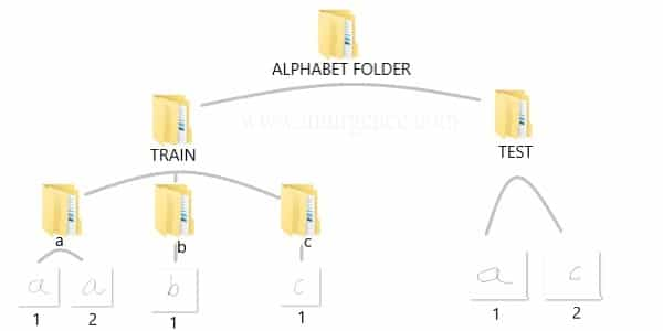
Image Source : From Author

You can download the data which I have used, right click on this download data link and open in new tab or window. Then unzip the folders and you should be able to see the same structure and data as above in your downloads folder. I would suggest, you should create your own data and repeat the  process. This would help you understand the complete flow.

Install the Dependency Packages for RStudio

We will be using the jpeg package in R for Image handling and the SVM implementation from the kernlab package.  Also we need to make sure that the image data has dimension’s of 200 x 200 pixels, with a horizontal and vertical resolution of 120dpi. You can vary the dimension’s like move it to 300 x 300 or reduce it to 100 x 100. The higher the dimension, you will need more compute power. Experiment around the color channels and resolution later once you have implemented it in the current form.

# install package "jpeg"

  install.packages("jpeg", dependencies = TRUE)


# install the "kernlab" package for building the model using support vector machines

install.packages("kernlab", dependencies  = TRUE)

Load the training data set

# load the "jpeg" package for reading the JPEG format files
library(jpeg)

# set the working directory for reading the training image data set
setwd("C:/Users/mohan/Desktop/alphabet_folder/Train")

# extract the directory names for using as image labels

f_train<-list.files()
 

# Create an empty data frame to store the image data labels and the extracted new features in training environment

df_train<- data.frame(matrix(nrow=0,ncol=5))

Feature Transformation

Since we don’t intend to use the typical CNN, we are going to use the white, grey and black pixel values for new feature creation. We will use the summation of all the pixel values of a image  and save it as a new feature called as “sum”, the count of all pixels adding up to zero as “zero”, the count of all pixels adding up to “ones” and the sum of all pixels between zero’s and one’s as “in_between”. The “label” feature names are extracted from the names of the folder

# names the columns of the data frame as per the feature name schema

names(df_train)<- c("sum","zero","one","in_between","label")

# loop to compute as per the logic

counter<-1 

for(i in 1:length(f_train))

{

setwd(paste("C:/Users/mohan/Desktop/alphabet_folder/Train/",f_train[i],sep=""))


data_list<-list.files()


  for(j in 1:length(data_list))

  {

    temp<- readJPEG(data_list[j])

    df_train[counter,1]<- sum(temp)

    df_train[counter,2]<- sum(temp==0)

    df_train[counter,3]<- sum(temp==1)

    df_train[counter,4]<- sum(temp > 0 & temp < 1)

    df_train[counter,5]<- f_train[i]

    counter=counter+1

  }

}


# Convert the labels from text to factor form

df_train$label<- factor(df_train$label)

Support Vector Machine model

# load the "kernlab" package for accessing the support vector machine implementation

library(kernlab)


# build the model using the training data

image_classifier <- ksvm(label~.,data=df_train)

Evaluate the Model on the Testing Data Set

# set the working directory for reading the testing image data set

setwd("C:/Users/mohan/Desktop/alphabet_folder/Test")


# extract the directory names for using as image labels

f_test <- list.files()

 
# Create an empty data frame to store the image data labels and the extracted new features in training environment

df_test<- data.frame(matrix(nrow=0,ncol=5))

 
# Repeat of feature extraction in test data

names(df_test)<- c("sum","zero","one","in_between","label")

 
# loop to compute as per the logic

for(i in 1:length(f_test))

{

temp<- readJPEG(f_test[i])

df_test[i,1]<- sum(temp)

df_test[i,2]<- sum(temp==0)

df_test[i,3]<- sum(temp==1)

df_train[counter,4]<- sum(temp > 0 & temp < 1)

df_test[i,5]<- strsplit(x = f_test[i],split = "[.]")[[1]][1]

}
 

# Use the classifier named "image_classifier" built in train environment to predict the outcomes on features in Test environment

df_test$label_predicted<- predict(image_classifier,df_test)
 

# Cross Tab for Classification Metric evaluation

table(Actual_data=df_test$label,Predicted_data=df_test$label_predicted) 

I would recommend you to learn concepts of SVM which couldn’t be explained completely in this article by going through my free Data Science and Machine Learning video courses. We have created the classifier using the Kerlab package in R, but I would advise you to study the mathematics involved in Support vector machines to get a clear understanding.

A common trap when it comes to sampling from a population that intrinsically includes outliers

I will discuss a common fallacy concerning the conclusions drawn from calculating a sample mean and a sample standard deviation and more importantly how to avoid it.

Suppose you draw a random sample x_1, x_2, … x_N of size N and compute the ordinary (arithmetic) sample mean  x_m and a sample standard deviation sd from it.  Now if (and only if) the (true) population mean µ (first moment) and population variance (second moment) obtained from the actual underlying PDF  are finite, the numbers x_m and sd make the usual sense otherwise they are misleading as will be shown by an example.

By the way: The common correlation coefficient will also be undefined (or in practice always point to zero) in the presence of infinite population variances. Hopefully I will create an article discussing this related fallacy in the near future where a suitable generalization to Lévy-stable variables will be proposed.

 Drawing a random sample from a heavy tailed distribution and discussing certain measures

As an example suppose you have a one dimensional random walker whose step length is distributed by a symmetric standard Cauchy distribution (Lorentz-profile) with heavy tails, i.e. an alpha-stable distribution with alpha being equal to one. The PDF of an individual independent step is given by p(x) = \frac{\pi^{-1}}{(1 + x^2)} , thus neither the first nor the second moment exist whereby the first exists and vanishes at least in the sense of a principal value due to symmetry.

Still let us generate N = 3000 
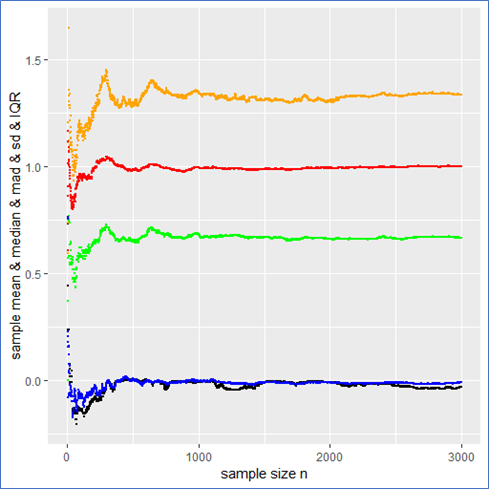
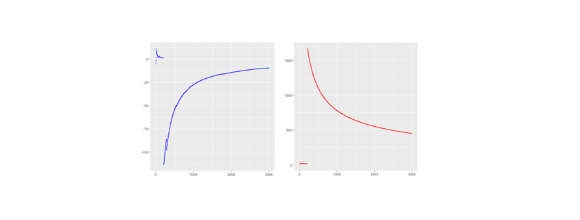
(pseudo) standard Cauchy random numbers in R* to analyze the behavior of their sample mean and standard deviation sd as a function of the reduced sample size n \leq N.

*The R-code is shown at the end of the article.

Here are the piecewise sample mean (in blue) and standard deviation (in red) for the mentioned Cauchy sampling. We see that both the sample mean and sd include jumps and do not converge.

Especially the mean deviates relatively largely from zero even after 3000 observations. The sample sd has no target due to the population variance being infinite.

If the data is new and no prior distribution is known, computing the sample mean and sd will be misleading. Astonishingly enough the sample mean itself will have the (formally exact) same distribution as the single step length p(x)
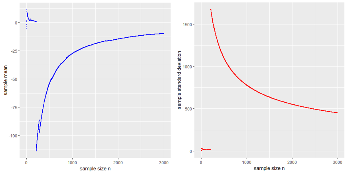
. This means that the sample mean is also standard Cauchy distributed implying that with a different Cauchy sample one could have easily observed different sample means far of the presented values in blue.

What sense does it make to present the usual interval x_m \pm sd / \sqrt{N} in such a case? What to do?

The sample median, median absolute difference (mad) and Inter-Quantile-Range (IQR) are more appropriate to describe such a data set including outliers intrinsically. To make this plausible I present the following plot, whereby the median is shown in black, the mad in green and the IQR in orange.

This example shows that the median, mad and IQR converge quickly against their assumed values and contain no major jumps. These quantities do an obviously better job in describing the sample. Even in the presence of outliers they remain robust, whereby the mad converges more quickly than the IQR. Note that a standard Cauchy sample will contain half of its sample in the interval median \pm 
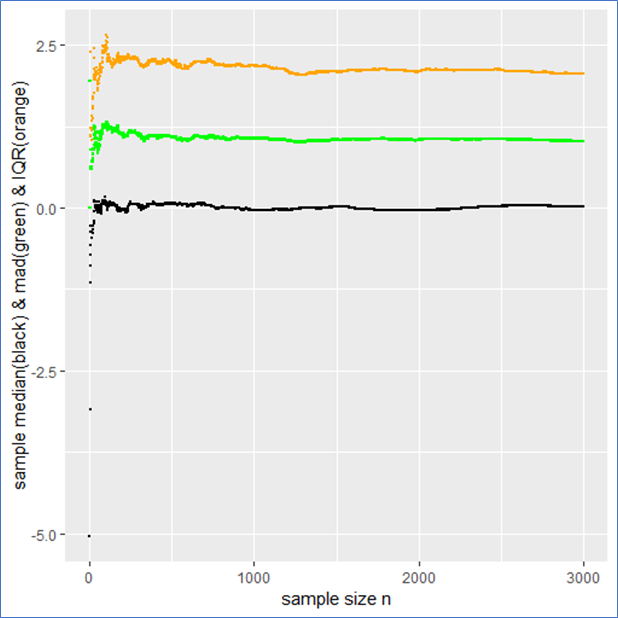
mad meaning that the IQR is twice the mad.

Drawing a random sample from a PDF that has finite moments

Just for comparison I also show the above quantities for a standard normal (pseudo) sample labeled with the same color as before as a counter example. In this case not only do both the sample mean and median but also the sd and mad converge towards their expected values (see plot below). Here all the quantities describe the data set properly and there is no trap since there are no intrinsic outliers. The sample mean itself follows a standard normal, so that the sd in deed makes sense and one could calculate a standard error \frac{sd}{\sqrt{N}} from it to present the usual stochastic confidence intervals for the sample mean.

A careful observation shows that in contrast to the Cauchy case here the sampled mean and sd converge more quickly than the sample median and the IQR. However still the sampled mad performs about as well as the sd. Again the mad is twice the IQR.

And here are the graphs of the prementioned quantities for a pseudo normal sample:

The take-home-message:

Just be careful when you observe outliers and calculate sample quantities right away, you might miss something. At best one carefully observes how the relevant quantities change with sample size as demonstrated in this article.

Such curves should become of broader interest in order to improve transparency in the Data Science process and reduce fallacies as well.

Thank you for reading.

P.S.: Feel free to play with the set random seed in the R-code below and observe how other quantities behave with rising sample size. Of course you can also try different PDFs at the beginning of the code. You can employ a Cauchy, Gaussian, uniform, exponential or Holtsmark (pseudo) random sample.


QUIZ: Which one of the recently mentioned random samples contains a trap** and why?

**in the context of this article


R-code used to generate the data and for producing plots:


#R-script for emphasizing convergence and divergence of sample means

####install and load relevant packages ####

#uncomment these lines if necessary
#install.packages(c('ggplot2',’stabledist’))
#library(ggplot2)
#library(stabledist)

#####drawing random samples #####

#Setting a random seed for being able to reproduce results  
set.seed(1234567)   
N= 2000     #sample size

#Choose a PDF from which a sample shall be drawn
#To do so (un)comment the respective lines of following code

data <- rcauchy(N)    # option1(default): standard Cauchy sampling

#data <- rnorm(N)     #option2: standard Gaussian sampling
                               
#data <- rexp(N)    # option3: standard exponential sampling

#data <- rstable(N,alpha=1.5,beta=0)  # option4: standard symmetric Holtsmark sampling

#data <- runif(N)              #option5: standard uniform sample

#####descriptive statistics####
#preparations/declarations

SUM = vector()
sd =vector()
mean = vector()
SQ =vector()
SQUARES = vector()
median = vector()
mad =vector()
quantiles = data.frame()
sem =vector()

#piecewise calculaion of descrptive quantities

for (k in 1:length(data)){              #mainloop
SUM[k] <- sum(data[1:k])            # sum of sample
mean[k] <- mean(data[1:k])          # arithmetic mean
sd[k] <- sd(data[1:k])              # standard deviation
sem[k] <- sd[k]/(sqrt(k))          #standard error of the sample mean (for finite variances)
mad[k] <- mad(data[1:k],const=1)   # median absolute deviation    

for (j in 1:5){
qq <- quantile(data[1:k],na.rm = T)
quantiles[k,j] <- qq[j]         #quantiles of sample
}
colnames(quantiles) <- c('min','Q1','median','Q3','max')

for (i in 1:length(data[1:k])){
SQUARES[i] <- data[i]*data[i]    
}
SQ[k] <- sum(SQUARES[1:k])    #sum of squares of random sample
}  #end of mainloop

#create table containing all relevant data
TABLE <-  as.data.frame(cbind(quantiles,mean,sd,SQ,SUM,sem))


#####plotting results###
x11()
print(ggplot(TABLE,aes(1:N,median))+
geom_point(size=.5)+xlab('sample size n')+ylab('sample median'))
x11()
print(ggplot(TABLE,aes(1:N,mad))+geom_point(size=.5,color ='green')+
xlab('sample size n')+ylab('sample median absolute difference'))
x11()
print(ggplot(TABLE,aes(1:N,sd))+geom_point(size=.5,color ='red')+
xlab('sample size n')+ylab('sample standard deviation'))
x11()
print(ggplot(TABLE,aes(1:N,mean))+geom_point(size=.5, color ='blue')+
xlab('sample size n')+ylab('sample mean'))
x11()
print(ggplot(TABLE,aes(1:N,Q3-Q1))+geom_point(size=.5, color ='blue')+
xlab('sample size n')+ylab('IQR'))

#uncomment the following lines of code to see further plots

#x11()
#print(ggplot(TABLE,aes(1:N,sem))+geom_point(size=.5)+
#xlab('sample size n')+ylab('sample sum of r.v.'))
#x11()
#print(ggplot(TABLE,aes(1:N,SUM))+geom_point(size=.5)+
#xlab('sample size n')+ylab('sample sum of r.v.'))
#x11()
#print(ggplot(TABLE,aes(1:N,SQ))+geom_point(size=.5)+
#xlab('sample size n')+ylab('sample sum of squares'))


Bringing intelligence to where data lives: Python & R embedded in T-SQL

Introduction

Did you know that you can write R and Python code within your T-SQL statements? Machine Learning Services in SQL Server eliminates the need for data movement. Instead of transferring large and sensitive data over the network or losing accuracy with sample csv files, you can have your R/Python code execute within your database. Easily deploy your R/Python code with SQL stored procedures making them accessible in your ETL processes or to any application. Train and store machine learning models in your database bringing intelligence to where your data lives.

You can install and run any of the latest open source R/Python packages to build Deep Learning and AI applications on large amounts of data in SQL Server. We also offer leading edge, high-performance algorithms in Microsoft’s RevoScaleR and RevoScalePy APIs. Using these with the latest innovations in the open source world allows you to bring unparalleled selection, performance, and scale to your applications.

If you are excited to try out SQL Server Machine Learning Services, check out the hands on tutorial below. If you do not have Machine Learning Services installed in SQL Server,you will first want to follow the getting started tutorial I published here: 

How-To Tutorial

In this tutorial, I will cover the basics of how to Execute R and Python in T-SQL statements. If you prefer learning through videos, I also published the tutorial on YouTube.

Basics

Open up SQL Server Management Studio and make a connection to your server. Open a new query and paste this basic example: (While I use Python in these samples, you can do everything with R as well)

EXEC sp_execute_external_script @language = N'Python',
@script = N'print(3+4)'

Sp_execute_external_script is a special system stored procedure that enables R and Python execution in SQL Server. There is a “language” parameter that allows us to choose between Python and R. There is a “script” parameter where we can paste R or Python code. If you do not see an output print 7, go back and review the setup steps in this article.

Parameter Introduction

Now that we discussed a basic example, let’s start adding more pieces:

EXEC sp_execute_external_script  @language =N'Python', 
@script = N' 
OutputDataSet = InputDataSet;
',
@input_data_1 =N'SELECT 1 AS Col1';

Machine Learning Services provides more natural communications between SQL and R/Python with an input data parameter that accepts any SQL query. The input parameter name is called “input_data_1”.
You can see in the python code that there are default variables defined to pass data between Python and SQL. The default variable names are “OutputDataSet” and “InputDataSet” You can change these default names like this example:

EXEC sp_execute_external_script  @language =N'Python', 
@script = N' 
MyOutput = MyInput;
',
@input_data_1_name = N'MyInput',
@input_data_1 =N'SELECT 1 AS foo',
@output_data_1_name =N'MyOutput';

As you executed these examples, you might have noticed that they each return a result with “(No column name)”? You can specify a name for the columns that are returned by adding the WITH RESULT SETS clause to the end of the statement which is a comma separated list of columns and their datatypes.

EXEC sp_execute_external_script  @language =N'Python', 
@script=N' 
MyOutput = MyInput;
',
@input_data_1_name = N'MyInput',
@input_data_1 =N'
SELECT 1 AS foo,
2 AS bar
',
@output_data_1_name =N'MyOutput'
WITH RESULT SETS ((MyColName int, MyColName2 int));

Input/Output Data Types

Alright, let’s discuss a little more about the input/output data types used between SQL and Python. Your input SQL SELECT statement passes a “Dataframe” to python relying on the Python Pandas package. Your output from Python back to SQL also needs to be in a Pandas Dataframe object. If you need to convert scalar values into a dataframe here is an example:

EXEC sp_execute_external_script  @language =N'Python', 
@script=N' 
import pandas as pd
c = 1/2
d = 1*2
s = pd.Series([c,d])
df = pd.DataFrame(s)
OutputDataSet = df
'

Variables c and d are both scalar values, which you can add to a pandas Series if you like, and then convert them to a pandas dataframe. This one shows a little bit more complicated example, go read up on the python pandas package documentation for more details and examples:

EXEC sp_execute_external_script  @language =N'Python', 
@script=N' 
import pandas as pd
s = {"col1": [1, 2], "col2": [3, 4]}
df = pd.DataFrame(s)
OutputDataSet = df
'

You now know the basics to execute Python in T-SQL!

Did you know you can also write your R and Python code in your favorite IDE like RStudio and Jupyter Notebooks and then remotely send the execution of that code to SQL Server? Check out these documentation links to learn more: https://aka.ms/R-RemoteSQLExecution https://aka.ms/PythonRemoteSQLExecution

Check out the SQL Server Machine Learning Services documentation page for more documentation, samples, and solutions. Check out these E2E tutorials on github as well.

Would love to hear from you! Leave a comment below to ask a question, or start a discussion!