Prerequisites for understanding RNN at a more mathematical level

Writing the A gentle introduction to the tiresome part of understanding RNN Article Series on recurrent neural network (RNN) is nothing like a creative or ingenious idea. It is quite an ordinary topic. But still I am going to write my own new article on this ordinary topic because I have been frustrated by lack of sufficient explanations on RNN for slow learners like me.

I think many of readers of articles on this website at least know that RNN is a type of neural network used for AI tasks, such as time series prediction, machine translation, and voice recognition. But if you do not understand how RNNs work, especially during its back propagation, this blog series is for you.

After reading this articles series, I think you will be able to understand RNN in more mathematical and abstract ways. But in case some of the readers are allergic or intolerant to mathematics, I tried to use as little mathematics as possible.

Ideal prerequisite knowledge:

• Some understanding on densely connected layers (or fully connected layers, multilayer perception) and how their forward/back propagation work.
•  Some understanding on structure of Convolutional Neural Network.

*In this article “Densely Connected Layers” is written as “DCL,” and “Convolutional Neural Network” as “CNN.”

1, Difficulty of Understanding RNN

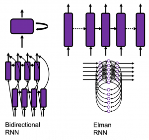
I bet a part of difficulty of understanding RNN comes from the variety of its structures. If you search “recurrent neural network” on Google Image or something, you will see what I mean. But that cannot be helped because RNN enables a variety of tasks.

Another major difficulty of understanding RNN is understanding its back propagation algorithm. I think some of you found it hard to understand chain rules in calculating back propagation of densely connected layers, where you have to make the most of linear algebra. And I have to say backprop of RNN, especially LSTM, is a monster of chain rules. I am planing to upload not only a blog post on RNN backprop, but also a presentation slides with animations to make it more understandable, in some external links.

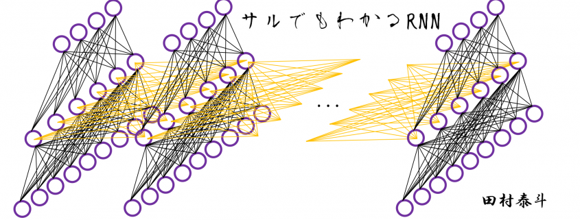
In order to avoid such confusions, I am going to introduce a very simplified type of RNN, which I call a “simple RNN.” The RNN displayed as the head image of this article is a simple RNN.

2, How Neurons are Connected

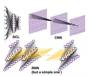
How to connect neurons and how to activate them is what neural networks are all about. Structures of those neurons are easy to grasp as long as that is about DCL or CNN. But when it comes to the structure of RNN, many study materials try to avoid showing that RNNs are also connections of neurons, as well as DCL or CNN(*If you are not sure how neurons are connected in CNN, this link should be helpful. Draw a random digit in the square at the corner.). In fact the structure of RNN is also the same, and as long as it is a simple RNN, and it is not hard to visualize its structure.

Even though RNN is also connections of neurons, usually most RNN charts are simplified, using blackboxes. In case of simple RNN, most study material would display it as the chart below.

But that also cannot be helped because fancier RNN have more complicated connections of neurons, and there are no longer advantages of displaying RNN as connections of neurons, and you would need to understand RNN in more abstract way, I mean, as you see in most of textbooks.

I am going to explain details of simple RNN in the next article of this series.

3, Neural Networks as Mappings

If you still think that neural networks are something like magical spider webs or models of brain tissues, forget that. They are just ordinary mappings.

If you have been allergic to mathematics in your life, you might have never heard of the word “mapping.” If so, at least please keep it in mind that the equation , which most people would have seen in compulsory education, is a part of mapping. If you get a value x, you get a value y corresponding to the x.

But in case of deep learning, x is a vector or a tensor, and it is denoted with . If you have never studied linear algebra , imagine that a vector is a column of Excel data (only one column), a matrix is a sheet of Excel data (with some rows and columns), and a tensor is some sheets of Excel data (each sheet does not necessarily contain only one column.)

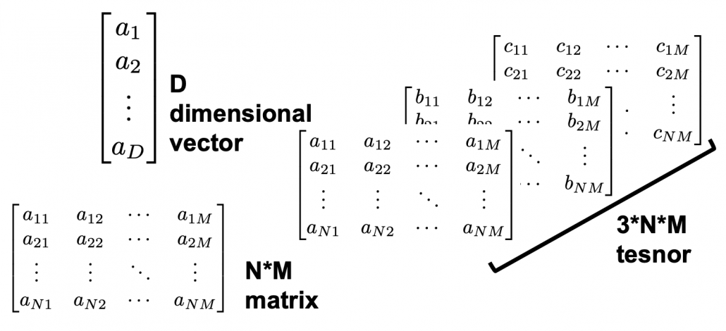
CNNs are mainly used for image processing, so their inputs are usually image data. Image data are in many cases (3, hight, width) tensors because usually an image has red, blue, green channels, and the image in each channel can be expressed as a hight*width matrix (the “height” and the “width” are number of pixels, so they are discrete numbers).

The convolutional part of CNN (which I call “feature extraction part”) maps the tensors to a vector, and the last part is usually DCL, which works as classifier/regressor. At the end of the feature extraction part, you get a vector. I call it a “semantic vector” because the vector has information of “meaning” of the input image. In this link you can see maps of pictures plotted depending on the semantic vector. You can see that even if the pictures are not necessarily close pixelwise, they are close in terms of the “meanings” of the images.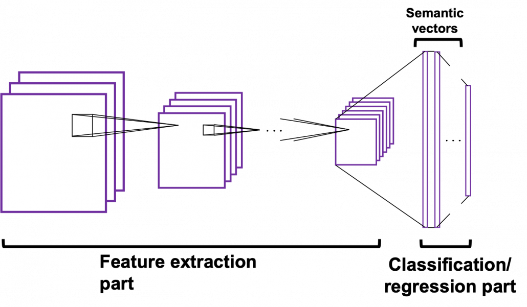

In the example of a dog/cat classifier introduced by François Chollet, the developer of Keras, the CNN maps (3, 150, 150) tensors to 2-dimensional vectors, (1, 0) or (0, 1) for (dog, cat).

Wrapping up the points above, at least you should keep two points in mind: first, DCL is a classifier or a regressor, and CNN is a feature extractor used for image processing. And another important thing is, feature extraction parts of CNNs map images to vectors which are more related to the “meaning” of the image.

Importantly, I would like you to understand RNN this way. An RNN is also just a mapping.

*I recommend you to at least take a look at the beautiful pictures in this link. These pictures give you some insight into how CNN perceive images.

4, Problems of DCL and CNN, and needs for RNN

Taking an example of RNN task should be helpful for this topic. Probably machine translation is the most famous application of RNN, and it is also a good example of showing why DCL and CNN are not proper for some tasks. Its algorithms is out of the scope of this article series, but it would give you a good insight of some features of RNN. I prepared three sentences in German, English, and Japanese, which have the same meaning. Assume that each sentence is divided into some parts as shown below and that each vector corresponds to each part. In machine translation we want to convert a set of the vectors into another set of vectors.

Then let’s see why DCL and CNN are not proper for such task.

• The input size is fixed: In case of the dog/cat classifier I have mentioned, even though the sizes of the input images varies, they were first molded into (3, 150, 150) tensors. But in machine translation, usually the length of the input is supposed to be flexible.
• The order of inputs does not mater: In case of the dog/cat classifier the last section, even if the input is “cat,” “cat,” “dog” or “dog,” “cat,” “cat” there’s no difference. And in case of DCL, the network is symmetric, so even if you shuffle inputs, as long as you shuffle all of the input data in the same way, the DCL give out the same outcome . And if you have learned at least one foreign language, it is easy to imagine that the orders of vectors in sequence data matter in machine translation.

*It is said English language has phrase structure grammar, on the other hand Japanese language has dependency grammar. In English, the orders of words are important, but in Japanese as long as the particles and conjugations are correct, the orders of words are very flexible. In my impression, German grammar is between them. As long as you put the verb at the second position and the cases of the words are correct, the orders are also relatively flexible.

5, Sequence Data

We can say DCL and CNN are not useful when you want to process sequence data. Sequence data are a type of data which are lists of vectors. And importantly, the orders of the vectors matter. The number of vectors in sequence data is usually called time steps. A simple example of sequence data is meteorological data measured at a spot every ten minutes, for instance temperature, air pressure, wind velocity, humidity. In this case the data is recorded as 4-dimensional vector every ten minutes.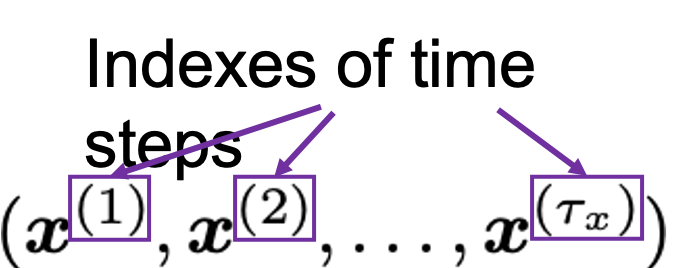

But this “time step” does not necessarily mean “time.” In case of natural language processing (including machine translation), which you I mentioned in the last section, the numberings of each vector denoting each part of sentences are “time steps.”

And RNNs are mappings from a sequence data to another sequence data.

*At least I found a paper on the RNN’s capability of universal approximation on many-to-one RNN task. But I have not found any papers on universal approximation of many-to-many RNN tasks. Please let me know if you find any clue on whether such approximation is possible. I am desperate to know that. 

6, Types of RNN Tasks

RNN tasks can be classified into some types depending on the lengths of input/output sequences (the “length” means the times steps of input/output sequence data).

If you want to predict the temperature in 24 hours, based on several time series data points in the last 96 hours, the task is many-to-one. If you sample data every ten minutes, the input size is 96*6=574 (the input data is a list of 574 vectors), and the output size is 1 (which is a value of temperature). Another example of many-to-one task is sentiment classification. If you want to judge whether a post on SNS is positive or negative, the input size is very flexible (the length of the post varies.) But the output size is one, which is (1, 0) or (0, 1), which denotes (positive, negative).

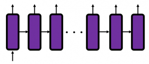
*The charts in this section are simplified model of RNN used for each task. Please keep it in mind that they are not 100% correct, but I tried to make them as exact as possible compared to those in other study materials.

Music/text generation can be one-to-many tasks. If you give the first sound/word you can generate a phrase.

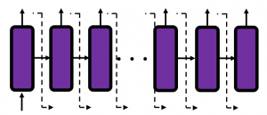
Next, let’s look at many-to-many tasks. Machine translation and voice recognition are likely to be major examples of many-to-many tasks, but here name entity recognition seems to be a proper choice. Name entity recognition is task of finding proper noun in a sentence . For example if you got two sentences “He said, ‘Teddy bears on sale!’ ” and ‘He said, “Teddy Roosevelt was a great president!” ‘ judging whether the “Teddy” is a proper noun or a normal noun is name entity recognition.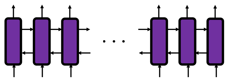

Machine translation and voice recognition, which are more popular, are also many-to-many tasks, but they use more sophisticated models. In case of machine translation, the inputs are sentences in the original language, and the outputs are sentences in another language. When it comes to voice recognition, the input is data of air pressure at several time steps, and the output is the recognized word or sentence. Again, these are out of the scope of this article but I would like to introduce the models briefly.

Machine translation uses a type of RNN named sequence-to-sequence model (which is often called seq2seq model). This model is also very important for other natural language processes tasks in general, such as text summarization. A seq2seq model is divided into the encoder part and the decoder part. The encoder gives out a hidden state vector and it used as the input of the decoder part. And decoder part generates texts, using the output of the last time step as the input of next time step.

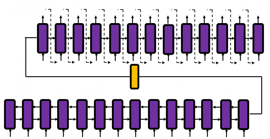
Voice recognition is also a famous application of RNN, but it also needs a special type of RNN.

*To be honest, I don’t know what is the state-of-the-art voice recognition algorithm. The example in this article is a combination of RNN and a collapsing function made using Connectionist Temporal Classification (CTC). In this model, the output of RNN is much longer than the recorded words or sentences, so a collapsing function reduces the output into next output with normal length.

You might have noticed that RNNs in the charts above are connected in both directions. Depending on the RNN tasks you need such bidirectional RNNs.  I think it is also easy to imagine that such networks are necessary. Again, machine translation is a good example.

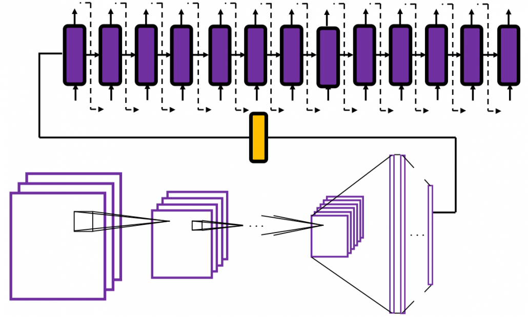
And interestingly, image captioning, which enables a computer to describe a picture, is one-to-many-task. As the output is a sentence, it is easy to imagine that the output is “many.” If it is a one-to-many task, the input is supposed to be a vector.

Where does the input come from? I told you that I was obsessed with the beauty of the last vector of the feature extraction part of CNN. Surprisingly the the “beautiful” vector, which I call a “semantic vector” is the input of image captioning task (after some transformations, depending on the network models).

I think this articles includes major things you need to know as prerequisites when you want to understand RNN at more mathematical level. In the next article, I would like to explain the structure of a simple RNN, and how it forward propagate.

* I make study materials on machine learning, sponsored by DATANOMIQ. I do my best to make my content as straightforward but as precise as possible. I include all of my reference sources. If you notice any mistakes in my materials, please let me know (email: yasuto.tamura@datanomiq.de). And if you have any advice for making my materials more understandable to learners, I would appreciate hearing it.

About Author

Yasuto Tamura

Data Science Intern at DATANOMIQ.
Majoring in computer science. Currently studying mathematical sides of deep learning, such as densely connected layers, CNN, RNN, autoencoders, and making study materials on them. Also started aiming at Bayesian deep learning algorithms.

See author's posts