Air Quality Forecasting Python Project
You will find the full python code and all visuals for this article here in this gitlab repository. The repository contains a series of analysis, transforms and forecasting models frequently used when dealing with time series. The aim of this repository is to showcase how to model time series from the scratch, for this we are using a real usecase dataset
This project forecast the Carbon Dioxide (Co2) emission levels yearly. Most of the organizations have to follow government norms with respect to Co2 emissions and they have to pay charges accordingly, so this project will forecast the Co2 levels so that organizations can follow the norms and pay in advance based on the forecasted values. In any data science project the main component is data, for this project the data was provided by the company, from here time series concept comes into the picture. The dataset for this project contains 215 entries and two components which are Year and Co2 emissions which is univariate time series as there is only one dependent variable Co2 which depends on time. from year 1800 to year 2014 Co2 levels were present in the dataset.
The dataset used: The dataset contains yearly Co2 emmisions levels. data from 1800 to 2014 sampled every 1 year. The dataset is non stationary so we have to use differenced time series for forecasting.
After getting data the next step is to analyze the time series data. This process is done by using Python. The data was present in excel file so first we need to read that excel file. This task is done by using Pandas which is python libraries to creates Pandas Data Frame. After that preprocessing like changing data types of time from object to DateTime performed for the coding purpose. Time series contain 4 main components Level, Trend, Seasonality and Noise. To study this component, we need to decompose our time series so that we can batter understand our time series and we can choose the forecasting model accordingly because each component behave different on the model. also by decomposing we can identify that the time series is multiplicative or additive.
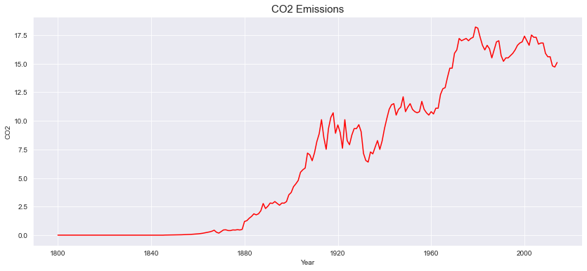
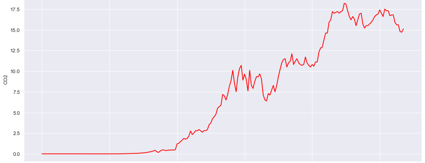
CO2 emissions – plotted via python pandas / matplotlib
Decomposing time series using python statesmodels libraries we get to know trend, seasonality and residual component separately. the components multiply together to make the time series multiplicative and in additive time series components added together. Taking the deep dive to understand the trend component, moving average of 10 steps were applied which shows nonlinear upward trend, fit the linear regression model to check the trend which shows upward trend. talking about seasonality there were combination of multiple patterns over time period which is common in real world time series data. capturing the white noise is difficult in this type of data. the time series contains values from 1800 where the Co2 values are less then 1 because of no human activities so levels were decreasing. By the time numbers of industries and human activities are rapidly increasing which causes Co2 levels rapidly increasing. In time series the highest Co2 emission level was 18.7 in 1979. It was challenging to decide whether to consider this values which are less then 0.5 as white noise or not because 30% of the Co2 values were less then 1, in real world looking at current scenario the chances of Co2 emission level being 0 is near to impossible still there are chances that Co2 levels can be 0.0005. So considering each data point as a valuable information we refused to remove that entries.
Next step is to create Lag plot so we can see the correlation between the current year Co2 level and previous year Co2 level. the plot was linear which shows high correlation so we can say that the current Co2 levels and previous levels have strong relationship. the randomness of the data were measured by plotting autocorrelation graph. the autocorrelation graph shows smooth curves which indicates the time series is non–stationary thus next step is to make time series stationary. in non–stationary time series, summary statistics like mean and variance change over time.
To make time series stationary we have to remove trend and seasonality from it. Before that we use dickey fuller test to make sure our time series is non–stationary. the test was done by using python, and the test gives p–value as output. here the null hypothesis is that the data is non–stationary while alternate hypothesis is that the data is stationary, in this case the significance values is 0.05 and the p–values which is given by dickey fuller test is greater than 0.05 hence we failed to reject null hypothesis so we can say the time series is non–stationery. Differencing is one of the techniques to make time series stationary. On this time series, first order differencing technique applied to make the time series stationary. In first order differencing we have to subtract previous value from current value for all the data points. also different transformations like log, sqrt and reciprocal were applied in the context of making the time series stationary. Smoothing techniques like simple moving average, exponential weighted moving average, simple exponential smoothing and double exponential smoothing techniques can be applied to remove the variation between time stamps and to see the smooth curves.
Smoothing techniques also used to observe trend in time series as well as to predict the future values. But performance of other models was good compared to smoothing techniques. First 200 entries taken to train the model and remaining last for testing the performance of the model. performance of different models measured by Root Mean Squared Error (RMSE) and Mean Absolute Error (MAE) as we are predicting future Co2 emissions so basically it is regression problem. RMSE is calculated by root of the average of squared difference between actual values and predicted values by the model on testing data. Here RMSE values were calculated using python sklearn library. For model building two approaches are there, one is data–driven and another one is model based. models from both the approaches were applied to find the best fitted model. ARIMA model gives the best results for this kind of dataset as the model were trained on differenced time series. The ARIMA model predicts a given time series based on its own past values. It can be used for any non–seasonal series of numbers that exhibits patterns and is not a series of random events. ARIMA takes 3 parameters which are AR, MA and the order of difference. Hyper parameter tuning technique gives best parameters for the model by trying different sets of parameters. Although The autocorrelation and partial autocorrelation plots can be use to decide AR and MA parameter because partial autocorrelation function shows the partial correlation of a stationary time series with its own lagged values so using PACF we can decide the value of AR and from ACF we can decide the value of MA parameter as ACF shows how data points in a time series are related.
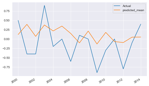
Yearly difference of CO2 emissions – ARIMA Prediction
Apart from ARIMA, few other model were trained which are AR, ARMA, Simple Linear Regression, Quadratic method, Holts winter exponential smoothing, Ridge and Lasso Regression, LGBM and XGboost methods, Recurrent neural network (RNN) – Long Short Term Memory (LSTM) and Fbprophet. I would like to mention my experience with LSTM here because it is another model which gives good result as ARIMA. the reason for not choosing LSTM as final model is its complexity. As ARIMA is giving appropriate results and it is simple to understand and requires less dependencies. while using lstm, lot of data preprocessing and other dependencies required, the dataset was small thus we used to train the model on CPU, otherwise gpu is required to train the LSTM model. we face one more challenge in deployment part. the challenge is to get the data into original form because the model was trained on differenced time series, so it will predict the future values in differenced format. After lot of research on the internet and by deeply understanding mathematical concepts finally we got the solution for it. solution for this issue is we have to add previous value from the original data from into first order differencing and then we have to add the last value of this time series into predicted values. To create the user interface streamlit was used, it is commonly used python library. the pickle file of the ARIMA model were used to predict the future values based on user input. The limit for forecasting is the year 2050. The project was uploaded on google cloud platform. so the flow is, first the starting year from which user want to forecast was taken and the end year till which year user want to forecast was taken and then according to the range of this inputs the prediction takes place. so by taking the inputs the pickle file will produce the future Co2 emissions in differenced format, then the values will be converted to original format and then the original values will be displayed on the user interface as well as the interactive line graph were displayed on the interface.
You will find the full python code and all visuals for this article here in this gitlab repository.