Geschriebene Artikel über Big Data Analytics

Statistical Relational Learning

An Introduction to Statistical Relational Learning – Part 1

Statistical Relational Learning (SRL) is an emerging field and one that is taking centre stage in the Data Science age. Big Data has been one of the primary reasons for the continued prominence of this relational learning approach given, the voluminous amount of data available now to learn interesting and unknown patterns from data. Moreover, the tools have also improved their processing prowess especially, in terms of scalability.

This introductory blog is a prelude on SRL and later on I would also touch base on more advanced topics, specifically Markov Logic Networks (MLN). To start off, let’s look at how SRL fits into one of the 5 different Machine Learning paradigms.

Five Machine Learning Paradigms

Lets look at the 5 Machine Learning Paradigms: Each of which is inspired by ideas from a different field!

  1. Connectionists as they are called and led by Geoffrey Hinton (University of Toronto & Google and one of the major names in the Deep Learning community) think that a learning algorithm should mimic the brain! After all it is the brain that does all the complex actions for us and, this idea stems from Neuroscience.
  2. Another group of Evolutionists whose leader is the late John Holland (from the University of Michigan) believed it is not the brain but evolution that was precedent and hence the master algorithm to build anything. And using this approach of having the fittest ones program the future they are currently building 3D prints of future robots.
  3. Another thought stems from Philosophy where Analogists like Douglas R. Hofstadter an American writer and author of popular and award winning book – Gödel, Escher, Bach: an Eternal Golden Braid believe that Analogy is the core of Cognition.
  4. Symbolists like Stephen Muggleton (Imperial College London) think Psychology is the base and by developing Rules in deductive reasoning they built Adam – a robot scientist at the University of Manchester!
  5. Lastly we have a school of thought which has its foundations rested on Statistics & Logic, which is the focal point of interest in this blog. This emerging field has started to gain prominence with the invention of Bayesian networks 2011 by Judea Pearl (University of California Los Angeles – UCLA) who was awarded with the Turing award (the highest award in Computer Science). Bayesians as they are called, are the most fanatical of the lot as they think everything can be represented by the Bayes theorem using hypothesis which can be updated based on new evidence.

SRL fits into the last paradigm of Statistics and Logic. As such it offers another alternative to the now booming Deep Learning approach inspired from Neuroscience.

Background

In many real world scenario and use cases, often the underlying data is assumed to be independent and identically distributed (i.i.d.). However, real world data is not and instead consists of many relationships. SRL as such attempts to represent, model, and learn in the relational domain!

There are 4 main Models in SRL

  1. Probabilistic Relational Models (PRM)
  2. Markov Logic Networks (MLN)
  3. Relational Dependency Networks (RDN)
  4. Bayesian Logic Programs (BLP)

It is difficult to cover all major models and hence the focus of this blog is only on the emerging field of Markov Logic Networks.
MLN is a powerful framework that combines statistics (i.e. it uses Markov Random Fields) and logical reasoning (first order logic).


markov-random-fields-first-order-logic

Academia

Some of the prominent names in academic and the research community in MLN include:

  1. Professor Pedro Domingos from the University of Washington is credited with introducing MLN in his paper from 2006. His group created the tool called Alchemy which was one of the first, First Order Logic tools.
  2. Another famous name – Professor Luc De Raedt from the AI group at University of Leuven in Belgium, and their team created the tool ProbLog which also has a Python Wrapper.
  3. HAZY Project (Stanford University) led by Prof. Christopher Ré from the InfoLab is doing active research in this field and Tuffy, Felix, Elementary, Deep Dive are some of the tools developed by them. More on it later!
  4. Talking about academia close by i.e. in Germany, Prof. Michael Beetz and his entire team moved from TUM to TU Bremen. Their group invented the tool – ProbCog
  5. At present, Prof. Volker Tresp from Ludwig Maximilians University (LMU), Munich & Dr. Matthias Nickles at Technical University of Munich (TUM) have research interests in SRL.

Theory & Formulation

A look at some background and theoretical concepts to understand MLN better.

A. Basics – Probabilistic Graphical Models (PGM)

The definition of a PGM goes as such:

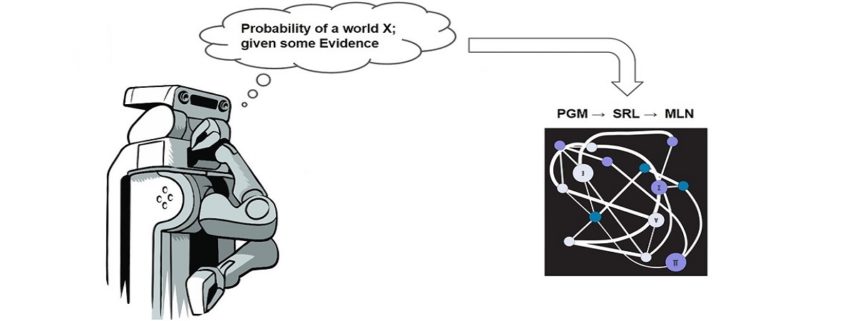
A PGM encodes a joint p(x,y) or conditional p(y|x) probability distribution such that given some observations we are provided with a full probability distribution over all feasible solutions.

A PGM helps to encode relationships between a set of random variables. And it achieves this by making use of a graph! These graphs can be either be Directed or Undirected Graphs.

B. Markov Blanket

A Markov Blanket is a Directed Acyclic graph. It is a Bayesian network and as you can see the central node A highlighted in red is dependent on its parents and parents of descendents (moralization) by the circle drawn around it. Thus these nodes are the only knowledge needed to predict node A.

C. Markov Random Fields (MRF)

A MRF is an Undirected graphical model. Every node in an MRF satisfies the Local Markov property of Conditional Independence, i.e. a node is conditionally independent of another node, given its neighbours. And now relating it to Markov Blanket as explained previously, a Markov blanket for a node is simply its adjacent nodes!

Intuition

We now that Probability handles uncertainty whereas Logic handles complexity. So why not make use of both of them to model relationships in data that is both uncertain and complex. Markov Logic Networks (MLN) precisely does that for us!

MLN is composed of a set of pairs of  <w, F> where F is the formula (written in FO logic) and weights (real numbers identifying the strength of the constraint).

MLN basically provides a template to ground a Markov network. Grounding would be explained in detail in the next but one section on “Weight Learning”.

It can be defined as a Log linear model where probability of a world is given by the weighted sum of all true groundings of a formula i under an exponential function. It is then divided by Z which is termed as the partition function and used to normalize and get probability values between 0 and 1.

propability_of_a_world_x

The MLN Template

Rules or Predicates

The relation to be learned is expressed in FO logic. Some of the different possible FO logical connectives and quantifiers are And (^), Or (V), Implication (→), and many more. Plus, Formulas may contain one or more predicates, connected to each other with logical connectives and quantified symbols.

Evidence

Evidence represent known facts i.e. the ground predicates. Each fact is expressed with predicates that contain only constants from their corresponding domains.

Weight Learning

Discover the importance of relations based on grounded evidence.

Inference

Query relations, given partial evidence to infer a probabilistic estimate of the world.

More on Weight Learning and Inference in the next part of this series!

Hope you enjoyed the read. I have deliberately kept the content basic and a mix of non technical and technical so as to highlight first the key players and some background concepts and generate the reader’s interest in this topic, the technicalities of which can easily be read in the paper. Any feedback as a comment below or through a message are more than welcome!

Continue reading with Statistical Relational Learning – Part II.

References

Data Science on a large scale – can it be done?

Analytics drives business

In today’s digital world, data has become the crucial success factor for businesses as they seek to maintain a competitive advantage, and there are numerous examples of how companies have found smart ways of monetizing data and deriving value accordingly.

On the one hand, many companies use data analytics to streamline production lines, optimize marketing channels, minimize logistics costs and improve customer retention rates.  These use cases are often described under the umbrella term of operational BI, where decisions are based on data to improve a company’s internal operations, whether that be a company in the manufacturing industry or an e-commerce platform.

On the other hand, over the last few years, a whole range of new service-oriented companies have popped up whose revenue models wholly depend on data analytics.  These Data-Driven Businesses have contributed largely to the ongoing development of new technologies that make it possible to process and analyze large amounts of data to find the right insights.  The better these technologies are leveraged, the better their value-add and the better for their business success.  Indeed, without data and data analytics, they don’t have a business.

Data Science – hype or has it always been around?Druck

In my opinion, there is too much buzz around the new era of data scientists.  Ten years ago, people simply called it data mining, describing similar skills and methods.  What has actually changed is the fact that businesses are now confronted with new types of data sources such as mobile devices and data-driven applications rather than statistical methodologies.  I described that idea in detail in my recent post Let’s replace the Vs of Big Data with a single D.

But, of course, you cannot deny that the importance of these data crunchers has increased significantly. The art of mining data mountains (or perhaps I should say “diving through data lakes”) to find appropriate insights and models and then find the right answers to urgent, business-critical questions has become very popular these days.

The challenge: Data Science with large volumes?

Michael Stonebraker, winner of the Turing Award 2014, has been quoted as saying: “The change will come when business analysts who work with SQL on large amounts of data give way to data EXASOL Pipelinescientists, which will involve more sophisticated analysis, predictive modeling, regressions and Bayesian classification. That stuff at scale doesn’t work well on anyone’s engine right now. If you want to do complex analytics on big data, you have a big problem right now.”

And if you look at the limitations of existing statistical environments out there using R, Python, Java, Julia and other languages, I think he is absolutely right.  Once the data scientists have to handle larger volumes, the tools are just not powerful and scalable enough.  This results in data sampling or aggregation to make statistical algorithms applicable at all.

A new architecture for “Big Data Science”

We at EXASOL have worked hard to develop a smart solution to respond to this challenge.  Imagine that it is possible to use raw data and intelligent statistical models on very large data sets, directly at the place where the data is stored.  Where the data is processed in-memory to achieve optimal performance, all distributed across a powerful MPP cluster of servers, in an environment where you can now “install” the programming language of your choice.

Sounds far-fetched?  If you are not convinced, then I highly recommend you have a look at our brand-new in-database analytic programming platform, which is deeply integrated in our parallel in-memory engine and extensible through using nearly any programming language and statistical library.

For further information on our approach to big data science, go ahead and download a copy of our technical whitepaper:  Big Data Science – The future of analytics.

Neural Nets: Time Series Prediction

Artificial neural networks are very strong universal approximators. Google recently defeated the worlds strongest Go (“chinese chess”) player with two neural nets, which captured the game board as a picture. Aside from these classification tasks, neural nets can be used to predict future values, behaviors or patterns solely based on learned history. In the machine learning literature, this is often referred to as time series prediction, because, you know, values over time need to be predicted. Hah! To illustrate the concept, we will train a neural net to learn the shape of a sinusoidal wave, so it can continue to draw the shape without any help. We will do this with Scala. Scala is a great lang, because it is strongly typed but feels easy like Python. Throughout this article, I will use the library NeuroFlow, which is a simple, lightweight library I wrote to build and train nets. Because Open Source is the way to go, feel free to check (and contribute to? :-)) the code on GitHub.

Introduction of the shape

If we, as humans, want to predict the future based on historic observations, we would have no other chance but to be guided by the shape drawn so far. Let’s study the plot below, asking ourselves: How would a human continue the plot?

sinuspredictdr
f(x) = sin(10*x)

Intuitively, we would keep on oscillating up and down, just like the grey dotted line tries to rough out. To us, the continuation of the shape is reasonably easy to understand, but a machine does not have a gut feeling to ask for a good guess. However, we can summon a Frankenstein, which will be able to learn and continue the shape based on numbers. In order to do so, let’s have a look at the raw, discrete data of our sinusoidal wave:

x f(x)
0.0 0.0
0.05 0.479425538604203
0.10 0.8414709848078965
0.15 0.9974949866040544
0.20 0.9092974268256817
0.25 0.5984721441039564
0.30 0.1411200080598672
0.35 -0.35078322768961984
0.75 0.9379999767747389

Ranging from 0.0 until 0.75, these discrete values drawn from our function with step size 0.05 will be the basis for training. Now, one could come up with the idea to just memorize all values, so a sufficiently reasonable value can be picked based on comparison. For instance, to continue at the point 0.75 in our plot, we could simply examine the area close to 0.15, noticing a similar value close to 1, and hence go downwards. Well, of course this is cheating, but if a good cheat is a superior solution, why not cheat? Being hackers, we wouldn’t care. What’s really limiting here is the fact that the whole data set needs to be kept in memory, which can be infeasible for large sets, plus for more complex shapes, this approach would quickly result in a lot of weird rules and exceptions to be made in order to find comprehensible predictions.

Net to the rescue

Let’s go back to our table and see if a neural net can learn the shape, instead of simply memorizing it. Here, we want our net architecture to be of kind [3, 5, 3, 1]. Three input neurons, two hidden layers with five and three neurons respectively, as well as one neuron for the output layer will capture the data shown in the table.

sinuspredictnet

A supervised training mode means, that we want to train our net with three discrete steps as input and the fourth step as the supervised training element. So we will train a, b, c -> d and e, f, g -> h et cetera, hoping that this way our net will capture the slope pattern of our sinusoidal wave. Let’s code this in Scala:

import neuroflow.core.Activator.Tanh 
import neuroflow.core.WeightProvider.randomWeights 
import neuroflow.nets.DynamicNetwork.constructor

First, we want a Tanh activation function, because the domain of our sinusoidal wave is [-1, 1], just like the hyperbolic tangent. This way we can be sure that we are not comparing apples with oranges. Further, we want a dynamic network (adaptive learning rate) and random initial weights. Let’s put this down:

val fn = Tanh.apply
val sets = Settings(true, 10.0, 0.0000001, 500, None, None, Some(Map("τ" -> 0.25, "c" -> 0.25)))
val net = Network(Input(3) :: Hidden(5, fn) :: Hidden(3, fn) :: Output(1, fn) :: Nil, sets)

No surprises here. After some experiments, we can pick values for the settings instance, which will promise good convergence during training. Now, let’s prepare our discrete steps drawn from the sinus function:

val group = 4
val sinusoidal = Range.Double(0.0, 0.8, 0.05).grouped(group).toList.map(i => i.map(k => (k, Math.sin(10 * k))))
val xsys = sinusoidal.map(s => (s.dropRight(1).map(_._2), s.takeRight(1).map(_._2)))
val xs = xsys.map(_._1)
val ys = xsys.map(_._2)
net.train(xs, ys)

We will draw samples from the range with step size 0.05. After this, we will construct our training values xs as well as our supervised output values ys. Here, a group consists of 4 steps, with 3 steps as input and the last step as the supervised value.

[INFO] [25.01.2016 14:07:51:677] [run-main-5] Taking step 499 - error: 1.4395661497489177E-4  , error per sample: 3.598915374372294E-5
[INFO] [25.01.2016 14:07:51:681] [run-main-5] Took 500 iterations of 500 with error 1.4304189739640242E-4  
[success] Total time: 4 s, completed 25.01.2016 14:20:56

After a pretty short time, we will see good news. Now, how can we check if our net can successfully predict the sinusoidal wave? We can’t simply call our net like a sinus function to map from one input value to one output value, e. g. something like net(0.75) == sin(0.75). Our net does not care about any x values, because it was trained purely based on the function values f(x), or the slope pattern in general. We need to feed our net with a three-dimensional input vector holding the first three, original function values to predict the fourth step, then drop the first original step and append the recently predicted step to predict the fifth step, et cetera. In other words, we need to traverse the net. Let’s code this:

val initial = Range.Double(0.0, 0.15, 0.05).zipWithIndex.map(p => (p._1, xs.head(p._2)))
val result = predict(net, xs.head, 0.15, initial)
result.foreach(r => println(s"${r._1}, ${r._2}"))

with

@tailrec def predict(net: Network, last: Seq[Double], i: Double, results: Seq[(Double, Double)]): Seq[(Double, Double)] = {
  if (i < 4.0) {
    val score = net.evaluate(last).head
    predict(net, last.drop(1) :+ score, i + 0.05, results :+ (i, score))
  } else results
}

So, basically we don’t just continue to draw the sinusoidal shape at the point 0.75, we draw the entire shape right from the start until 4.0 – solely based on our trained net! Now, let’s see how our Frankenstein will complete the sinusoidal shape from 0.75 on:

sinuspredictfintwo

I’d say, pretty neat? Keep in mind, here, the discrete predictions are connected through splines. Another interesting property of our trained net is its prediction compared to the original sinus function when taking the limit towards 4.0. Let’s plot both:

sinuspredictfin

The purple line is the original sinusoidal wave, whereas the green line is the prediction of our net. The first steps show great consistency, but slowly the curves diverge a little over time, as uncertainties will add up. To keep this divergence rather low, one could fine tune settings, for instance numeric precision. However, if one is taking the limit towards infinity, a perfect fit is illusory.

Final thoughts

That’s it! We have trained our net to learn and continue the sinusoidal shape. Now, I know that this is a rather academic example, but to train a neural net to learn more complex shapes is straightforward from here.

Thanks for reading!

A quick primer on TensorFlow – Google’s machine learning workhorse

Introducing Google Brains‘ TensorFlow™

This week started with major news for the machine learning and data science community: the Google Brain Team announced the open sourcing of TensorFlow, their numerical library for tensor network computations. This software is actively developed (and used!) within Google and builds on many of Google’s large scale neural network applications such as automatic image labeling and captioning as well as the speech recognition in Google’s apps.

TensorFlow in bullet points

Here are the main features:

  • Supports deep neural networks – and much more machine learning approaches
  • Highly scalable across many machines and huge data sets
  • Runs on desktops, servers, in cloud and even mobile devices
  • Computation can run on CPUs, GPUs or both
  • All this flexibility is covered by a single API making the execution very streamlined
  • Available interfaces: C++ and Python. More will follow (Java, R, Lua, Go…)
  • Comes with many tools helping to build and visualize the data flow networks
  • Includes a powerful gradient based optimizer with auto-differentiation
  • Extensible with C++
  • Usable for commercial applications – released under Apache Software Licence 2.0

Tensor, what? Tensor, why?

„Numerical library for tensor network computations“ maybe doesn’t sound too exciting, but let’s  consider the implications.

Application of tensors and their networks is a relatively new (but fast evolving) approach in machine learning. Tensors, if you recall your algebra classes, are simply n-dimensional data arrays (so a scalar is a 0th order tensor, a vector is 1st order, and a matrix a 2nd order matrix).

A simple practical example of is color image’s RGB layers (essentially three 2D matrices combined into a 3rd order tensor). Or a more business minded example – if your data source generates a table (a 2D array) every hour, you can look at the full data set as a 3rd order tensor – time being the extra dimension.

Tensor networks then represent “data flow graphs”, where the edges are your multi-dimensional data sets and nodes are the mathematical operations on this data.

Example of of a data flow graph with multiple nodes (data operations). Notice how the execution of nodes is asynchronous. This allows incredible scalability across many machines. Image Source.

Looking at your data through the tensor formalism gives you a lot of powerful tools that were already developed for tensor algebra, allowing fast, complex computations.  

Tensor networks are also a natural fit for computations done on graphical processing units (GPUs) as they are built exactly for the purpose of very fast numerical operations on such a data – speeding up your calculations significantly compared to standard CPU execution!

The importance of flexible architecture & scaling

The data flow graph approach has also further advantages. Most notably, you can split the design of your data flows (i.e. data cleaning, processing, transformations, model building etc.) from its execution. You first build up the graph of your data flow and then you send it to for execution: either on the CPUs of your machines (and it can be your laptop just as well as cluster) or GPUs or a combination. This happens through a single interface that hides all the complexities from you.

Since the execution is asynchronous it scales across many machines and can deal with huge amounts of data.

You can count on the Google guys to build tools not only for academic use, but also heavy-duty operations in the industry!

Is this just another deep learning library?

TensorFlow is of course not the first library to embrace the tensor formalism and GPU execution. The nearest comparisons (and competitors) are Theano, Torch and CGT (Caffe to a limited degree).

While there are significant overlaps between the libraries, TensorFlow tries to provide a broader framework. It is not only a deep learning library – the Data Flow Graphs can incorporate any data processing/analysis applications. It also comes with a very powerful gradient based optimizer with automatic calculations of derivatives offering huge flexibility.

Given this broad vision the closest competitor is probably Theano (while Caffe and the existing Theano wrappers have a narrower focus on deep learning). TensorFlow’s distinguishing feature is that by design its focus is on large, scalable architectures with a complete flexibility in the hardware, best suited for industry/operational use, whereas the other libraries have more academic pedigrees.

Initial analyses also indicate that TensorFlow should bring also performance improvements compared to Theano, although no comprehensive benchmarks have yet been published.

As the other packages are out already for a while, they have large, active communities and often additional supporting software (examples are the very useful wrappers around Theano like Lasagne, Keras and Blocks that provider higher level abstractions to its engine).

Of course, with Google’s gravitas, one can expect that TensorFlow’s open source community will grow very fast and the contributors will quickly add a lot of additional features (and find hidden bugs).

Finally, keep in mind, that while Google provided us with this great data processing framework and some of its machine learning capabilities, it is likely that the most powerful machine learning algorithms still remain Google’s proprietary secret.

Nonetheless, TensorFlow is a huge and very welcome contribution to the open source machine learning world!

Where to go next?

You can find Google’s getting started guide here. The TensorFlow white paper is worth a read too. Source code can be found at the Github page. There is also a Vagrant virtual machine with TensorFlow pre-installed available here.