Die Notwendigkeit von DevOps in Data Science

Datenwissenschaft und maschinelles Lernen werden häufig mit Mathematik, Statistik, Algorithmen und Datenstreitigkeiten in Verbindung gebracht. Während diese Fähigkeiten für den Erfolg der Implementierung von maschinellem Lernen in einem Unternehmen von zentraler Bedeutung sind, gewinnt eine Funktion zunehmend an Bedeutung – DevOps for Data Science. DevOps umfasst die Bereitstellung der Infrastruktur, das Konfigurationsmanagement, die kontinuierliche Integration und Bereitstellung, das Testen und die Überwachung. Die DevOps Consulting – Teams haben eng mit den Entwicklungsteams zusammengearbeitet, um den Lebenszyklus von Anwendungen effektiv zu verwalten.

Data Science bringt DevOps zusätzliche Verantwortung. Data Engineering, eine Nischendomäne, die sich mit komplexen Pipelines befasst, die die Daten transformieren, erfordert eine enge Zusammenarbeit von Data Science-Teams mit DevOps. Datenwissenschaftler untersuchen transformierte Daten, um Erkenntnisse und Korrelationen zu finden. Von den DevOps-Teams wird erwartet, dass sie Datenwissenschaftler unterstützen, indem sie Umgebungen für die Datenexploration und -visualisierung erstellen.

Das Erstellen von Modellen für maschinelles Lernen unterscheidet sich grundlegend von der herkömmlichen Anwendungsentwicklung. Die Entwicklung ist nicht nur iterativ, sondern auch heterogen. Datenwissenschaftler und -entwickler verwenden eine Vielzahl von Sprachen, Bibliotheken, Toolkits und Entwicklungsumgebungen, um Modelle für maschinelles Lernen zu entwickeln. Beliebte Sprachen für die Entwicklung des maschinellen Lernens wie Python, R und Julia werden in Entwicklungsumgebungen verwendet, die auf Jupyter Notebooks, PyCharm, Visual Studio Code, RStudio und Juno basieren. Diese Umgebungen müssen Datenwissenschaftlern und Entwicklern zur Verfügung stehen, die ML-Probleme lösen.

Maschinelles Lernen und Deep Learning erfordern eine massive Computerinfrastruktur, die auf leistungsstarken CPUs und GPUs ausgeführt wird. Frameworks wie TensorFlow, Caffe, Apache MXNet und Microsoft CNTK nutzen die GPUs, um komplexe Berechnungen für das Training von ML-Modellen durchzuführen. Das Bereitstellen, Konfigurieren, Skalieren und Verwalten dieser Cluster ist eine typische DevOps-Funktion. DevOps-Teams müssen möglicherweise Skripts erstellen, um die Bereitstellung und Konfiguration der Infrastruktur für eine Vielzahl von Umgebungen zu automatisieren.

Ähnlich wie bei der modernen Anwendungsentwicklung ist die Entwicklung des maschinellen Lernens iterativ.

Wenn ein vollständig trainiertes ML-Modell verfügbar ist, wird von DevOps-Teams erwartet, dass sie das Modell in einer skalierbaren Umgebung hosten, beispielsweise mit Microsoft Azure und die dazugehörige DevOps-Lösung. Sie können Orchestrierungs-Engines wie Apache Mesos oder Kubernetes nutzen, um die Modellbereitstellung zu skalieren.

DevOps-Teams nutzen Container für die Bereitstellung von Entwicklungsumgebungen, Datenverarbeitungs-Pipelines, Schulungsinfrastrukturen und Modellbereitstellungsumgebungen. Neue Technologien wie Kubeflow und MlFlow konzentrieren sich darauf, DevOps-Teams in die Lage zu versetzen, die neuen Herausforderungen im Umgang mit der ML-Infrastruktur zu bewältigen.

Maschinelles Lernen verleiht DevOps eine neue Dimension. Zusammen mit den Entwicklern müssen die Betreiber mit Datenwissenschaftlern und Dateningenieuren zusammenarbeiten, um Unternehmen zu unterstützen, die das ML-Paradigma annehmen.

Positional encoding, residual connections, padding masks: covering the rest of Transformer components

This is the fourth article of my article series named “Instructions on Transformer for people outside NLP field, but with examples of NLP.”

1 Wrapping points up so far

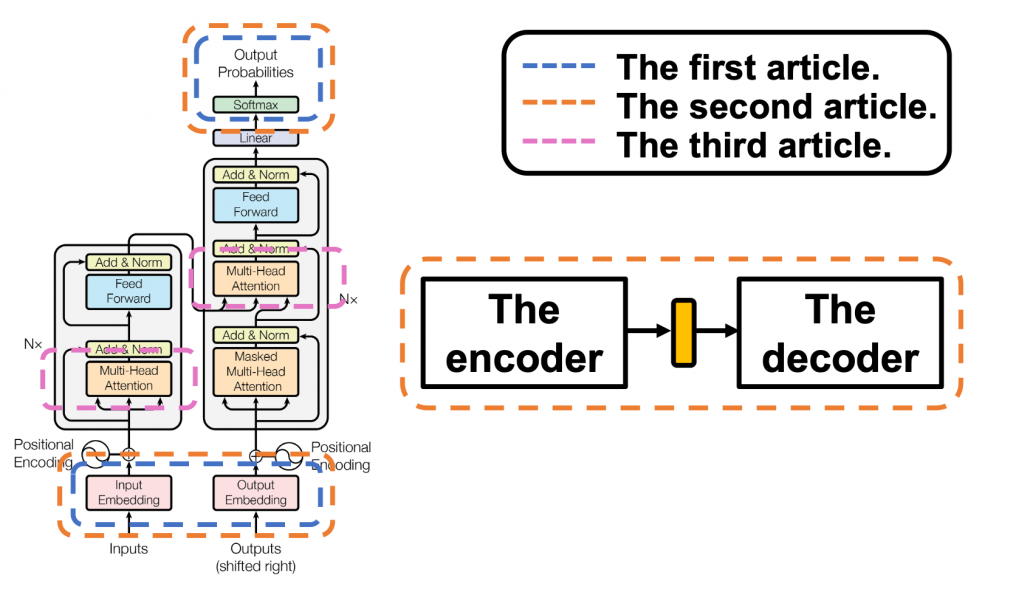
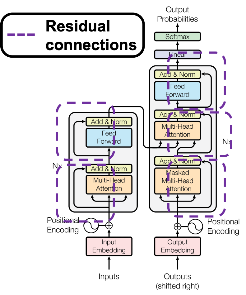
This article series has already covered a great deal of the Transformer mechanism. Whether you have read my former articles or not, I bet you are more or less lost in the course of learning Transformer model. The left side of the figure below is from the original paper on Transformer model, and my previous articles explained the parts in each colored frame. In the first article, I  mainly explained how language is encoded in deep learning task and how that is evaluated.

This is more of a matter of inputs and the outputs of deep learning networks, which are in blue dotted frames in the figure. They are not so dependent on types of deep learning NLP tasks. In the second article, I explained seq2seq models, which are encoder-decoder models used in machine translation. Seq2seq models can can be simplified like the figure in the orange frame. In the article I mainly explained seq2seq models with RNNs, but the purpose of this article series is ultimately replace them with Transformer models. In the last article, I finally wrote about some actual components of Transformer models: multi-head attention mechanism. I think this mechanism is the core of Transformed models, and I did my best to explain it with a whole single article, with a lot of visualizations. However, there are still many elements I have not explained.

First, you need to do positional encoding to the word embedding so that Transformer models can learn the relations of the positions of input tokens. At least I was too stupid to understand what this is only with the original paper on Transformer. I am going to explain this algorithm in illustrative ways, which I needed to self-teach it. The second point is residual connections.

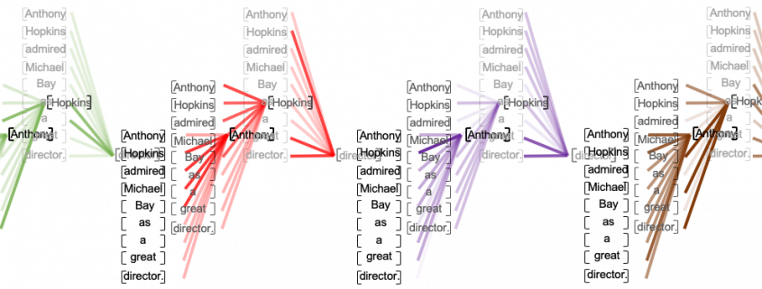
The last article has already explained multi-head attention, as precisely as I could do, but I still have to say I covered only two multi-head attention parts in a layer of Transformer model, which are in pink frames. During training, you have to mask some tokens at the decoder part so that some of tokens are invisible, and masked multi-head attention enables that.

You might be tired of the words “queries,” “keys,” and “values,” if you read the last article. But in fact that was not enough. When you think about applying Transformer in other tasks, such as object detection or image generation, you need to reconsider what the structure of data and how “queries,” “keys,” and “values,” correspond to each elements of the data, and probably one of my upcoming articles would cover this topic.

2 Why Transformer?

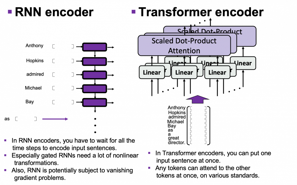
One powerful strength of Transformer model is its parallelization. As you saw in the last article, Trasformer models enable calculating relations of tokens to all other tokens, on different standards, independently in each head. And each head requires very simple linear transformations. In case of RNN encoders, if an input has \tau tokens, basically you have to wait for \tau time steps to finish encoding the input sentence. Also, at the time step (\tau) the RNN cell retains the information at the time step (1) only via recurrent connections. In this way you cannot attend to tokens in the earlier time steps, and this is obviously far from how we compare tokens in a sentence. You can bring information backward by bidirectional connection s in RNN models, but that all the more deteriorate parallelization of the model. And possessing information via recurrent connections, like a telephone game, potentially has risks of vanishing gradient problems. Gated RNN, such as LSTM or GRU mitigate the problems by a lot of nonlinear functions, but that adds to computational costs. If you understand multi-head attention mechanism, I think you can see that Transformer solves those problems.

I guess this is closer to when you speak a foreign language which you are fluent in. You wan to say something in a foreign language, and you put the original sentence in your mother tongue in the “encoder” in your brain. And you decode it, word by word, in the foreign language. You do not have to wait for the word at the end in your language, or rather you have to consider the relations of of a chunk of words to another chunk of words, in forward and backward ways. This is crucial especially when Japanese people speak English. You have to make the conclusion clear in English usually with the second word, but the conclusion is usually at the end of the sentence in Japanese.

3 Positional encoding

I explained disadvantages of RNN in the last section, but RNN has been a standard algorithm of neural machine translation. As I mentioned in the fourth section of the first article of my series on RNN, other neural nets like fully connected layers or convolutional neural networks cannot handle sequence data well. I would say RNN could be one of the only algorithms to handle sequence data, including natural language data, in more of classical methods of time series data processing.

*As I explained in this article, the original idea of RNN was first proposed in 1997, and I would say the way it factorizes time series data is very classical, and you would see similar procedures in many other algorithms. I think Transformer is a successful breakthrough which gave up the idea of processing sequence data time step by time step.

You might have noticed that multi-head attention mechanism does not explicitly uses the the information of the orders or position of input data, as it basically calculates only the products of matrices. In the case where the input is “Anthony Hopkins admired Michael Bay as a great director.”, multi head attention mechanism does not uses the information that “Hopkins” is the second token, or the information that the token two time steps later is “Michael.” Transformer tackles this problem with an almost magical algorithm named positional encoding.

In order to learn positional encoding, you should first think about what kind of encoding is ideal. According to this blog post, ideal encoding of positions of tokens have the following features.

  • Positional encoding of one token deterministically represents the position of the token.
  • The actual values of positional encoding should not be too big compared to the values of elements of embedding vectors.
  • Positional encodings of different tokens should successfully express their relative positions.

The most straightforward way to give the information of position is implementing the index of times steps (t), but if you naively give the term (t) to the data, the term could get too big compared to the values of data ,for example when the sequence data is 100 time steps long. The next straightforward idea is compressing the idea of time steps to for example the range [0, 1]. With this approach, however, the resolution of encodings can vary depending on the length of the input sequence data. Thus these naive approaches do not meet the requirements above, and I guess even conventional RNN-based models were not so successful in these points.

*I guess that is why attention mechanism of RNN seq2seq models, which I explained in the second article, was successful. You can constantly calculate the relative positions of decoder tokens compared to the encoder tokens.

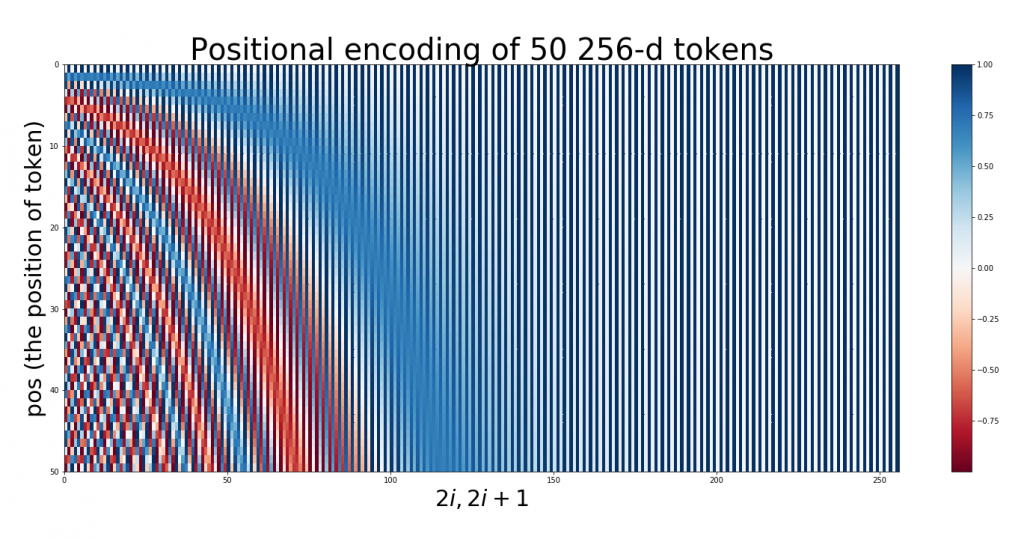
Positional encoding, to me almost magically, meets the points I have mentioned. However the explanation of positional encoding in the original paper of Transformer is unkindly brief. It says you can encode positions of tokens with the following vector PE_{(pos, 2i)} = sin(pos / 10000^{2i/d_model}), PE_{(pos, 2i+1)} = cos(pos / 10000^{2i/d_model}), where i = 0, 1, \dots, d_{model}/2 - 1. d_{model} is the dimension of word embedding. The heat map below is the most typical type of visualization of positional encoding you would see everywhere, and in this case d_{model}=256, and pos is discrete number which varies from 0 to 49, thus the heat map blow is equal to a 50\times 256 matrix, whose elements are from -1 to 1. Each row of the graph corresponds to one token, and you can see that lower dimensional part is constantly changing like waves. Also it is quite easy to encode an input with this positional encoding: assume that you have a matrix of an input sentence composed of 50 tokens, each of which is a 256 dimensional vector, then all you have to do is just adding the heat map below to the matrix.

Concretely writing down, the encoding of the 256-dim token at pos  is (PE_{(pos, 0)}, PE_{(pos, 1)}, \dots ,  PE_{(pos, 254)}, PE_{(pos, 255)})^T = \bigl( sin(pos / 10000^{0/256}), cos(pos / 10000^{0/256}) \bigr),  \dots , \bigl( sin(pos / 10000^{254/256}), cos(pos / 10000^{254/256}) \bigr)^T.

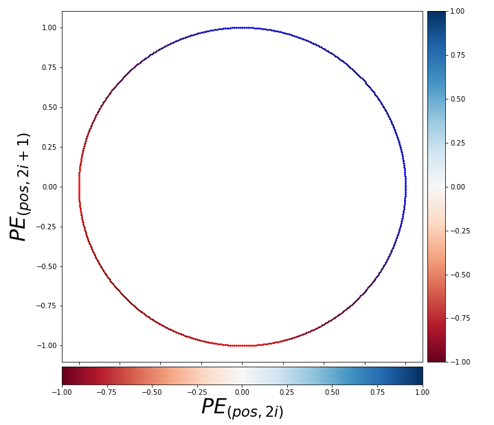
You should see this encoding more as d_{model} / 2 pairs of circles rather than d_{model} dimensional vectors. When you fix the i, the index of the depth of each encoding, you can extract a 2 dimensional vector \boldsymbol{PE}_i = \bigl( sin(pos / 10000^{2i/d_model}), cos(pos / 10000^{2i/d_model}) \bigr). If you constantly change the value pos, the vector \boldsymbol{PE}_i rotates clockwise on the unit circle in the figure below.

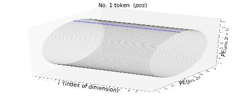
Also, the deeper the dimension of the embedding is, I mean the bigger the index i is, the smaller the frequency of rotation is. I think the video below is a more intuitive way to see how each token is encoded with positional encoding. You can see that the bigger pos is, that is the more tokens an input has, the deeper part positional encoding starts to rotate on the circles.


Very importantly, the original paper of Transformer says, “We chose this function because we hypothesized it would allow the model to easily learn to attend by relative positions, since for any fixed offset k, PE_{pos+k} can be represented as a linear function of PE_{pos}.” For each circle at any depth, I mean for any i, the following simple equation holds:

\left( \begin{array}{c} sin(\frac{pos+k}{10000^{2i/d_{model}}}) \\ cos(\frac{pos+k}{10000^{2i/d_{model}}}) \end{array} \right) =
\left( \begin{array}{ccc} cos(\frac{k}{10000^{2i/d_{model}}}) & sin(\frac{k}{10000^{2i/d_{model}}}) \\ -sin(\frac{k}{10000^{2i/d_{model}}}) & cos(\frac{k}{10000^{2i/d_{model}}}) \\ \end{array} \right) \cdot \left( \begin{array}{c} sin(\frac{pos}{10000^{2i/d_{model}}}) \\ cos(\frac{pos}{10000^{2i/d_{model}}}) \end{array} \right)

The matrix is a simple rotation matrix, so if i is fixed the rotation only depends on k, how many positions to move forward or backward. Then we get a very important fact: as the pos changes (pos is a discrete number), each point rotates in proportion to the offset of “pos,” with different frequencies depending on the depth of the circles. The deeper the circle is, the smaller the frequency is. That means, this type of positional encoding encourages Transformer models to learn definite and relative positions of tokens with rotations of those circles, and the values of each element of the rotation matrices are from -1 to 1, so they do not get bigger no matter how many tokens inputs have.

For example when an input is “Anthony Hopkins admired Michael Bay as a great director.”, a shift from the token “Hopkins” to “Bay” is a rotation matrix  \left( \begin{array}{ccc} cos(\frac{k}{10000^{2i/d_{model}}}) & sin(\frac{k}{10000^{2i/d_{model}}}) \\ -sin(\frac{k}{10000^{2i/d_{model}}}) & cos(\frac{k}{10000^{2i/d_{model}}}) \\ \end{array} \right), where k=3. Also the shift from “Bay” to “great” has the same rotation.

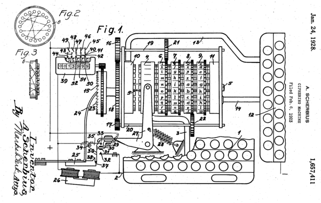
*Positional encoding reminded me of Enigma, a notorious cipher machine used by Nazi Germany. It maps alphabets to different alphabets with different rotating gear connected by cables. With constantly changing gears and keys, it changed countless patterns of alphabetical mappings, every day, which is impossible for humans to solve. One of the first form of computers was invented to break Enigma.

*As far as I could understand from “Imitation Game (2014).”

*But I would say Enigma only relied on discrete deterministic algebraic mapping of alphabets. The rotations of positional encoding is not that tricky as Enigma, but it can encode both definite and deterministic positions of much more variety of tokens. Or rather I would say AI algorithms developed enough to learn such encodings with subtle numerical changes, and I am sure development of NLP increased the possibility of breaking the Turing test in the future.

5 Residual connections

If you naively stack neural networks with simple implementation, that would suffer from vanishing gradient problems during training. Back propagation is basically multiplying many gradients, so

One way to mitigate vanishing gradient problems is quite easy: you have only to make a bypass of propagation. You would find a lot of good explanations on residual connections, so I am not going to explain how this is effective for vanishing gradient problems in this article.

In Transformer models you add positional encodings to the input only in the first layer, but I assume that the encodings remain through the layers by these bypass routes, and that might be one of reasons why Transformer models can retain information of positions of tokens.

6 Masked multi-head attention

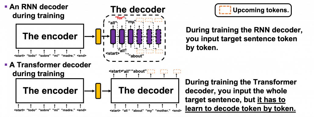
Even though Transformer, unlike RNN, can attend to the whole input sentence at once, the decoding process of Transformer-based translator is close to RNN-based one, and you are going to see that more clearly in the codes in the next article. As I explained in the second article, RNN decoders decode each token only based on the tokens the have generated so far. Transformer decoder also predicts the output sequences autoregressively one token at a time step, just as RNN decoders. I think it easy to understand this process because RNN decoder generates tokens just as you connect RNN cells one after another, like connecting rings to a chain. In this way it is easy to make sure that generating of one token in only affected by the former tokens. On the other hand, during training Transformer decoders, you input the whole sentence at once. That means Transformer decoders can see the whole sentence during training. That is as if a student preparing for a French translation test could look at the whole answer French sentences. It is easy to imagine that you cannot prepare for the French test effectively if you study this way. Transformer decoders also have to learn to decode only based on the tokens they have generated so far.

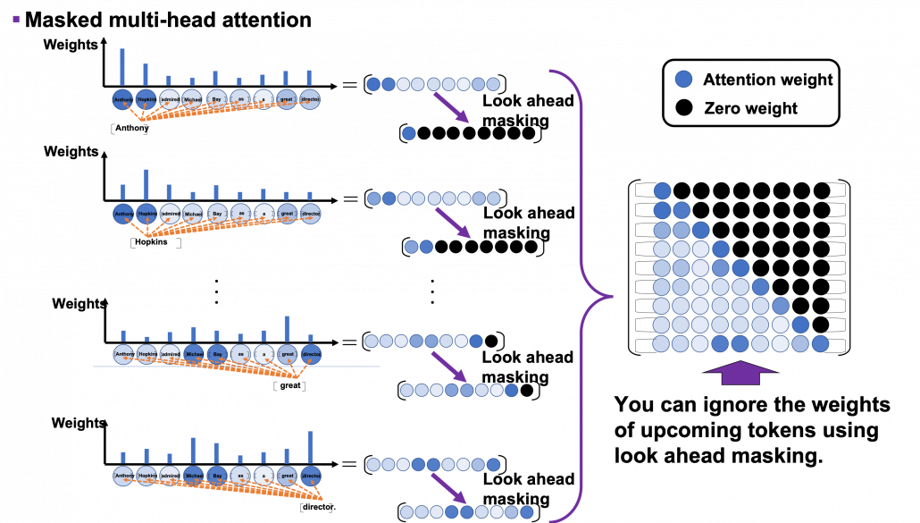
In order to properly train a Transformer-based translator to learn such decoding, you have to hide the upcoming tokens in target sentences during training. During calculating multi-head attentions in each Transformer layer, if you keep ignoring the weights from up coming tokens like in the figure below, it is likely that Transformer models learn to decode only based on the tokens generated so far. This is called masked multi-head attention.

*I am going to take an input “Anthonly Hopkins admire Michael Bay as a great director.” as an example of calculating masked multi-head attention mechanism, but this is supposed to be in the target laguage. So when you train an translator from English to German, in practice you have to calculate masked multi-head atetntion of “Anthony Hopkins hat Michael Bay als einen großartigen Regisseur bewundert.”

As you can see from the whole architecture of Transformer, you only need to consider masked multi-head attentions of of self-attentions of the input sentences at the decoder side. In order to concretely calculate masked multi-head attentions, you need a technique named look ahead masking. This is also quite simple. Just as well as the last article, let’s take an example of calculating self attentions of an input “Anthony Hopkins admired Michael Bay as a great director.” Also in this case you just calculate multi-head attention as usual, but when you get the histograms below, you apply look ahead masking to each histogram and delete the weights from the future tokens. In the figure below the black dots denote zero, and the sum of each row of the resulting attention map is also one. In other words, you get a lower triangular matrix, the sum of whose each row is 1.

Also just as I explained in the last article, you reweight vlaues with the triangular attention map. The figure below is calculating a transposed masked multi-head attention because I think it is a more straightforward way to see how vectors are reweighted in multi-head attention mechanism.

When you closely look at how each column of the transposed multi-head attention is reweighted, you can clearly see that the token is reweighted only based on the tokens generated so far.

*If you are still not sure why you need such masking in multi-head attention of target sentences, you should proceed to the next article for now. Once you check the decoding processes of Transformer-based translators, you would see why you need masked multi-head attention mechanism on the target sentence during training.

If you have read my articles, at least this one and the last one, I think you have gained more or less clear insights into how each component of Transfomer model works. You might have realized that each components require simple calculations. Combined with the fact that multi-head attention mechanism is highly parallelizable, Transformer is easier to train, compared to RNN.

In this article, we are going to see how masking of multi-head attention is implemented and how the whole Transformer structure is constructed. By the end of the next article, you would be able to create a toy English-German translator with more or less clear understanding on its architecture.

Appendix

You can visualize positional encoding the way I explained with simple Python codes below. Please just copy and paste them, importing necessary libraries. You can visualize positional encoding as both heat maps and points rotating on rings, and in this case the dimension of word embedding is 256, and the maximum length of sentences is 50.

# I borrowed this code from Tensorflow official tutorial. 
# https://www.tensorflow.org/tutorials/text/transformer

import matplotlib as mpl
from mpl_toolkits.mplot3d import Axes3D
import numpy as np
import matplotlib.pyplot as plt
from matplotlib import cm

def get_angles(pos, i, d_model):
  angle_rates = 1 / np.power(10000, (2 * (i//2)) / np.float32(d_model))
  return pos * angle_rates

def positional_encoding(position, d_model):
  angle_rads = get_angles(np.arange(position)[:, np.newaxis],
                          np.arange(d_model)[np.newaxis, :],
                          d_model)

  # apply sin to even indices in the array; 2i
  angle_rads[:, 0::2] = np.sin(angle_rads[:, 0::2])

  # apply cos to odd indices in the array; 2i+1
  angle_rads[:, 1::2] = np.cos(angle_rads[:, 1::2])

  pos_encoding = angle_rads[np.newaxis, ...]

  return pos_encoding.astype(np.float32)

resolution = 50
d_model = 256

n, d = resolution, d_model
pos_encoding = positional_encoding(n, d)
pos_encoding = pos_encoding[0]

plt.figure(figsize=(25, 10))
plt.pcolormesh(pos_encoding, cmap='RdBu')
plt.gca().invert_yaxis()
plt.ylabel('pos (the position of token)', fontsize=30)
plt.xlabel('2i, 2i+1', fontsize=30)
plt.colorbar()
plt.title("Positional encoding of 50 256-d tokens", fontsize=40)
plt.savefig("positional_encoding_heat_map.png")
plt.show()


import matplotlib as mpl
from mpl_toolkits.mplot3d import Axes3D
import numpy as np
import matplotlib.pyplot as plt
from matplotlib import cm

def get_angles(pos, i, d_model):
  angle_rates = 1 / np.power(10000, (2 * (i//2)) / np.float32(d_model))
  return pos * angle_rates

def positional_encoding(position, d_model):
  angle_rads = get_angles(np.arange(position)[:, np.newaxis],
                          np.arange(d_model)[np.newaxis, :],
                          d_model)

  # apply sin to even indices in the array; 2i
  angle_rads[:, 0::2] = np.sin(angle_rads[:, 0::2])

  # apply cos to odd indices in the array; 2i+1
  angle_rads[:, 1::2] = np.cos(angle_rads[:, 1::2])

  pos_encoding = angle_rads[np.newaxis, ...]

  return pos_encoding.astype(np.float32)


# A function to mix blue and red colors. 
def blue_red_gradation(x, y):
    red = np.array([1.0, 0.0, 0.0])
    blue = np.array([0.0, 0.0, 1.0])
    combined_color_x = (max(0, x)*blue + abs(min(x, 0))*red)/(abs(x) + abs(y))
    combined_color_y = (max(0, y)*blue + abs(min(y, 0))*red)/(abs(x) + abs(y))
    combined_color = (combined_color_x*abs(x) + combined_color_y*abs(y))/(abs(x) + abs(y))
    return combined_color[np.newaxis, ...]


resolution = 50
d_model = 256
x_range = 512
x_coordinates = np.linspace(0, d_model//2 - 1, d_model//2)
radius = 1
angular_velocity = np.pi / 12
y_coordinates = radius*np.cos(np.linspace(0, 1, resolution)*2*np.pi)
z_coordinates = radius*np.sin(np.linspace(0, 1, resolution)*2*np.pi)


n, d = resolution, d_model
pos_encoding = positional_encoding(n, d)
pos_encoding = pos_encoding[0]


#ax = fig.add_subplot(1, 1, 1, projection='3d')
color_vec = [[1., 0., 1.]]

markersize = 1
for j in range(resolution):
#for j in range(5):
    fig = plt.figure(figsize=(25, 10))
    ax = fig.gca(projection='3d')
    for i in range(d_model//2):
        ax.plot(x_coordinates[i]*np.ones(len(y_coordinates)), y_coordinates, z_coordinates, c='black', alpha=0.2)
    
    
    for i in range(len(x_coordinates)):
        ax.scatter(x_coordinates[i], radius*pos_encoding[:, 0::2][j, i], radius*pos_encoding[:, 1::2][j, i], 
                   c=blue_red_gradation(pos_encoding[:, 0::2][j, i], pos_encoding[:, 1::2][j, i]), alpha=0.5, s=20)
        ax.grid(False)

    ax.set_title(r'No. {} token  (pos)'.format(j+1), fontsize=40)
    ax.set_xlabel(r"i  (index of dimension)", fontsize=40)
    ax.set_ylabel(r'PE_{(pos, 2i)}', fontsize=40)
    ax.set_zlabel(r'PE_{(pos, 2i+1)}', fontsize=40)
    ax.set_xticks(np.arange(0, d_model//2, 10))
    plt.subplots_adjust(left=0, right=1, bottom=0, top=1)
    #plt.savefig('./positional_encoding_gif/{}.png'.format(j+1))
    plt.show()


*In fact some implementations use different type of positional encoding, as you can see in the codes below. In this case, embedding vectors are roughly divided into two parts, and each part is encoded with different sine waves. I have been using a metaphor of rotating rings or gears in this article to explain positional encoding, but to be honest that is not necessarily true of all the types of Transformer implementation. Some papers compare different types of pairs of positional encoding. The most important point is, Transformer models is navigated to learn positions of tokens with certain types of mathematical patterns.

[References]

[1] Ashish Vaswani, Noam Shazeer, Niki Parmar, Jakob Uszkoreit, Llion Jones, Aidan N. Gomez, Lukasz Kaiser, Illia Polosukhin, “Attention Is All You Need” (2017)

[2] “Transformer model for language understanding,” Tensorflow Core
https://www.tensorflow.org/overview

[3] Jay Alammar, “The Illustrated Transformer,”
http://jalammar.github.io/illustrated-transformer/

[4] “Stanford CS224N: NLP with Deep Learning | Winter 2019 | Lecture 14 – Transformers and Self-Attention,” stanfordonline, (2019)
https://www.youtube.com/watch?v=5vcj8kSwBCY

[5]Harada Tatsuya, “Machine Learning Professional Series: Image Recognition,” (2017), pp. 191-193
原田達也 著, 「機械学習プロフェッショナルシリーズ 画像認識」, (2017), pp. 191-193

[6] Amirhossein Kazemnejad, “Transformer Architecture: The Positional Encoding
Let’s use sinusoidal functions to inject the order of words in our model”, Amirhossein Kazemnejad’s Blog, (2019)
https://kazemnejad.com/blog/transformer_architecture_positional_encoding/

[7] Nicolas Carion, Francisco Massa, Gabriel Synnaeve, Nicolas Usunier, Alexander Kirillov, Sergey Zagoruyko, “End-to-End Object Detection with Transformers,” (2020)

[8]中西 啓、「【第5回】機械式暗号機の傑作~エニグマ登場~」、HH News & Reports, (2011)
https://www.hummingheads.co.jp/reports/series/ser01/110714.html

[9]中西 啓、「【第6回】エニグマ解読~第2次世界大戦とコンピュータの誕生~」、HH News & Reports, (2011)

[10]Tsuboi Yuuta, Unno Yuuya, Suzuki Jun, “Machine Learning Professional Series: Natural Language Processing with Deep Learning,” (2017), pp. 91-94
坪井祐太、海野裕也、鈴木潤 著, 「機械学習プロフェッショナルシリーズ 深層学習による自然言語処理」, (2017), pp. 191-193

[11]”Stanford CS224N: NLP with Deep Learning | Winter 2019 | Lecture 8 – Translation, Seq2Seq, Attention”, stanfordonline, (2019)
https://www.youtube.com/watch?v=XXtpJxZBa2c

* I make study materials on machine learning, sponsored by DATANOMIQ. I do my best to make my content as straightforward but as precise as possible. I include all of my reference sources. If you notice any mistakes in my materials, including grammatical errors, please let me know (email: yasuto.tamura@datanomiq.de). And if you have any advice for making my materials more understandable to learners, I would appreciate hearing it.


How Data Science Is Helping to Detect Child Abuse

Image Source: pixabay.com

There is no good way to begin a conversation about child abuse or neglect. It is a sad and oftentimes sickening topic. But the fact of the matter is it exists in our world today and frequently goes unnoticed or unreported, leaving many children and young adults to suffer. Of the nearly 3.6 million events that do get reported, there are rarely enough resources to go around for thorough follow up investigations.

This means that at least some objective decisions have to be made by professionals in the field. These individuals must assess reports, review, and ultimately decide which cases to prioritize for investigation on a higher level, which ones are probably nothing, and which ones are worrisome but don’t quite meet the definition of abuse or neglect.

Overall, it can be a challenging job that wears on a person, and one that many think is highly based on subjective information and bias. Because of this, numerous data researchers have worked to develop risk assessment models that can help these professionals discover hidden patterns and/or biases and make more informed decisions.

Defining the Work Space

Defining exactly what falls under the category of child abuse or neglect can be a surprisingly sticky topic. Broadly, it means anything that causes lasting physical or mental harm to children and young adults or negligence that could potentially harm or threaten a child’s wellbeing. What exactly constitutes child abuse can depend upon the state you live in.

Ultimately, a lot of the defining aspects are gray. Does spanking count as physical abuse or is the line drawn when it becomes hitting with a closed fist? Likewise, are parents negligent if they must leave their kids home alone to go to work? Does living in poverty automatically make people bad parents because there may not always be enough food in the house?

Sadly, many of these questions have become more prevalent during the COVID-19 pandemic. With many families cooped up at home together, not going to work or to school, kids who live in violent households are more likely to be abused and fewer people are seeing the children regularly to observe and report signs of abuse. Unfortunately, limited statistical data is available at this point, but with so many people having lost jobs, especially amongst families that may have already been teetering on the edge of poverty, situations that could be defined as neglectful are thought to be exploding in prevalence.

Identifying Patterns

The idea of using data science to help determine the risk of abuse and neglect that many children face can be seen by many as a powerful means of tackling a difficult issue. Much like many other aspects of our world today — data has become a very useful and highly valued commodity that can work to help us understand some of the deeper or hidden patterns.

That is exactly what has been incorporated in Allegheny County, Pennsylvania. The algorithm that was developed assesses the “risk factor” for each maltreatment allegation that is made in the county. The system takes into account several factors including mental health and drug treatment services, criminal histories, past calls, and more. All of this ultimately adds up to helping employees take into account how at-risk a child may actually be and whether or not the case will be prioritized for further investigation. Generalized reports indicate that the program works well, but that even it can ‘learn’ to make decisions based on bias.

In this situation, the goal of the program isn’t to take all of the power away from the employees but rather to work as a tool to help them make a sounder decision. Some risk factors will automatically be referred to a case handler for further investigation, but most will allow for the case assessor to weigh the algorithm with research and other information that may not be well accounted for in the model. If there are significant differences between the case assessor’s conclusion and the model’s conclusion, a supervisor reviews the information and makes the final decision.

Dealing with Bias

Of course, using a model such as this one can be a double-edged sword. Certain things are difficult to account for. For instance, if parents take financial advantage of their children by using their clean Social SecuNumbers to open credit cards and other credit accounts, their children can then be saddled with poor credit they did not create. Because this type of financial abuse is difficult to prove, it can be difficult for young adults to repair their credit later in life or hold their parents or guardians responsible. And the algorithm may struggle to recognize this as abuse. But it can also take out some of the bias that many of the call takers can inadvertently have when they are assessing the risk level of certain cases. A difference in conclusion from the model can force them to take a second look at the hard facts.

But there is a flip side. All models are created based on some level of personal decisions from the algorithm designer — those decisions can carry into biases that get carried into the model’s outputs. For example, the Alleghany County model has come under significant scrutiny for being biased against people who are living in poverty and using government programs to get by.

Because some of the major components the model uses to assess risk are public data, statistically, more people who rely on government programs are likely to be flagged regardless of how serious a call that comes in appears. Whereas families in the upper and middle class with private health insurance, drug treatment centers, and food security may be less likely to be picked up.

***

Big data can play a profound role in our lives and has the potential to be a powerful tool in helping identify and address child abuse cases. The available models can aid caseworkers in prioritizing risk assessments for further investigation and make a difference in the lives of children that are facing unacceptable situations. Being aware of and working to address any biases in models is an ongoing issue and those that aid in child abuse detection are no exception. Ultimately, if used correctly, this can be a powerful tool.

Seq2seq models and simple attention mechanism: backbones of NLP tasks

This is the second article of my article series “Instructions on Transformer for people outside NLP field, but with examples of NLP.”

1 Machine translation and seq2seq models

I think machine translation is one of the most iconic and commercialized tasks of NLP. With modern machine translation you can translate relatively complicated sentences, if you tolerate some grammatical errors. As I mentioned in the third article of my series on RNN, research on machine translation already started in the early 1950s, and their focus was translation between English and Russian, highly motivated by Cold War. In the initial phase, machine translation was rule-based, like most students do in their foreign language classes. They just implemented a lot of rules for translations. In the next phase, machine translation was statistics-based. They achieved better performance with statistics for constructing sentences. At any rate, both of them highly relied on feature engineering, I mean, you need to consider numerous rules of translation and manually implement them. After those endeavors of machine translation, neural machine translation appeared. The advent of neural machine translation was an earthshaking change of machine translation field. Neural machine translation soon outperformed the conventional techniques, and it is still state of the art. Some of you might felt that machine translation became more or less reliable around that time.

Source: Monty Python’s Life of Brian (1979)

I think you have learnt at least one foreign or classical language in school. I don’t know how good you were at the classes, but I think you had to learn some conjugations of them and I believe that was tiresome to most of students. For example, as a foreign person, I still cannot use “der”, “die”, “das” properly. Some of my friends recommended I do not care them for the time being while I speak, but I usually care grammar very much. But this method of learning language is close to the rule base machine translation, and modern neural machine translation basically does not rely on such rules.

As far as I understand, machine translation is pattern recognition learned from a large corpus. Basically no one implicitly teach computers how grammar works. Machine translation learns very complicated mapping from a source language to a target language, based on a lot of examples of word or sentence pairs. I am not sure, but this might be close to how bilingual kids learn how the two languages are related. You do not need to navigate the translator to learn specific grammatical rules.

Source: Monty Python’s Flying Circus (1969)

Since machine translation does not rely on manually programming grammatical rules, basically you do not need to prepare another specific network architecture for another pair of languages. The same method can be applied to any pairs of languages, as long as you have an enough size of corpus for that. You do not have to think about translation rules between other pairs of languages.

Source: Monty Python’s Flying Circus (1969)

*I do not follow the cutting edge studies on machine translation, so I am not sure, but I guess there are some heuristic methods for machine translation. That is, designing a network depending on the pair of languages could be effective. When it comes grammatical word orders, English and Japanese have totally different structures, I mean English is basically SVO and Japanese is basically SOV. In many cases, the structures of sentences with the same meaning in both of the languages are almost like reflections in a mirror. A lot of languages have similar structures to English, even in Asia, for example Chinese. On the other hand relatively few languages have Japanese-like structures, for example Korean, Turkish. I guess there would be some grammatical-structure-aware machine translation networks.

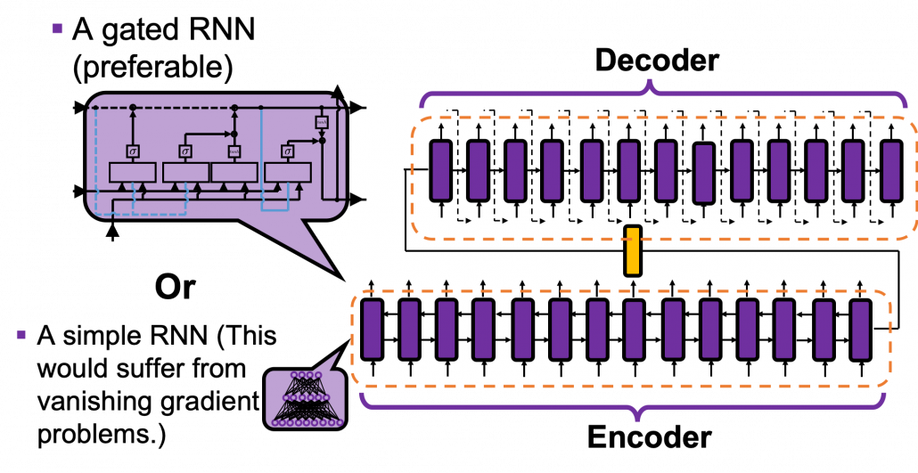
Not only machine translations, but also several other NLP tasks, such as summarization, question answering, use a model named seq2seq model (sequence to sequence model). As well as other deep learning techniques, seq2seq models are composed of an encoder and a decoder. In the case of seq2seq models, you use RNNs in both the encoder and decoder parts. For the RNN cells, you usually use a gated RNN such as LSTM or GRU because simple RNNs would suffer from vanishing gradient problem when inputs or outputs are long, and those in translation tasks are long enough. In the encoder part, you just pass input sentences. To be exact, you input them from the first time step to the last time step, every time giving an output, and passing information to the next cell via recurrent connections.

*I think you would be confused without some understandings on how RNNs propagate forward. You do not need to understand this part that much if you just want to learn Transformer. In order to learn Transformer model, attention mechanism, which I explain in the next section is more important. If you want to know how basic RNNs work, an article of mine should help you.

*In the encoder part of the figure below, the cell also propagate information backward. I assumed an encoder part with bidirectional RNNs, and they “forward propagate” information backwards. But in the codes below, we do not consider such complex situation. Please just keep it in mind that seq2seq model could use bidirectional RNNs.

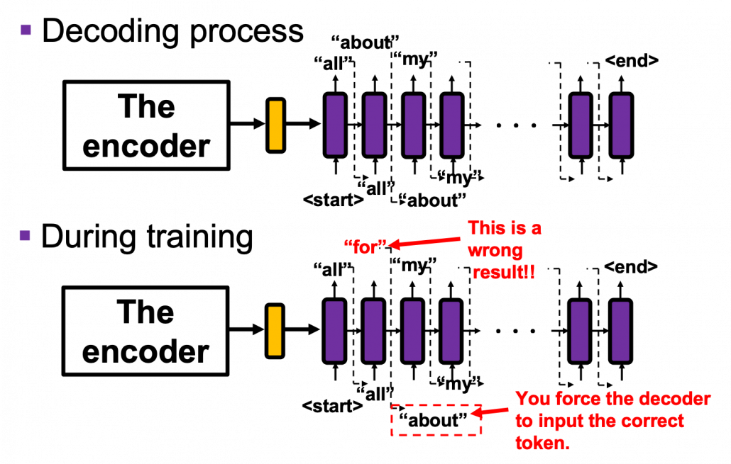
At the last time step in the encoder part, you pass the hidden state of the RNN to the decoder part, which I show as a yellow cell in the figure below, and the yellow cell/layer is the initial hidden layer of the first RNN cell of the decoder part. Just as normal RNNs, the decoder part start giving out outputs, and passing information via reccurent connections. At every time step you choose a token to give out from the vocabulary you use in the task. That means, each cell of decoder RNNs does a classification task and decides which word to write out at the time step. Also, very importantly, in the decoder part, the output at one time step is the input at the next time step, as I show as dotted lines in the figure below.

*The translation algorithm I explained depends on greedy decoding, which has to decide a token at every time step. However it is easy to imagine that that is not how you translate a word. You usually erase the earlier words or you construct some possibilities in your mind. Actually, for better translations you would need decoding strategies such as beam search, but it is out of the scope of at least this article. Thus we are going to make a very simplified translator based on greedy decoding.

2 Learning by making

*It would take some hours on your computer to train the translator if you do not use a GPU. I recommend you to run it at first and continue reading this article.

Seq2seq models do not have that complicated structures, and for now you just need to understand the points I mentioned above. Rather than just formulating the models, I think it would be better to understand this model by actually writing codes. If you copy and paste the codes in this Github page or the official Tensorflow tutorial, installing necessary libraries, it would start training the seq2seq model for Spanish-English translator. In the Github page, I just added comments to the codes in the official tutorial so that they are more understandable. If you can understand the codes in the tutorial without difficulty, I have to say this article itself is not compatible to your level. Otherwise, I am going to help you understand the tutorial with my original figures. I made this article so that it would help you read the next article. If you have no idea what RNN is, at least the second article of my RNN series should be helpful to some extent.

*If you try to read the the whole article series of mine on RNN, I think you should get prepared. I mean, you should prepare some pieces of paper and a pen. It would be nice if you have some stocks of coffee and snacks. Though I do not think you have to do that to read this article.

2.1 The corpus and datasets

In the codes in the Github page, please ignore the part sandwiched by “######”.  Handling language data is not the focus of this article. All you have to know is that the codes below first create datasets from the Spanish-English corpus in http://www.manythings.org/anki/ , and you datasets for training the translator as the tensors below.

Each token is encoded with integers as the codes below, thus after encoding, the Spanish sentence “Todo sobre mi madre.” is [1, 74, 514, 19, 237, 3, 2].

2.2 The encoder

The encoder part is relatively simple. All you have to keep in mind is that you put input sentences, and pass the hidden layer of the last cell to the decoder part. To be more concrete, an RNN cell receives an input word every time step, and gives out an output vector at each time step, passing hidden states to the next cell. You make a chain of RNN cells by the process, like in the figure below. In this case “time steps” means the indexes of the order of the words. If you more or less understand how RNNs work, I think this is nothing difficult. The encoder part passes the hidden state, which is in yellow in the figure below, to the decoder part.

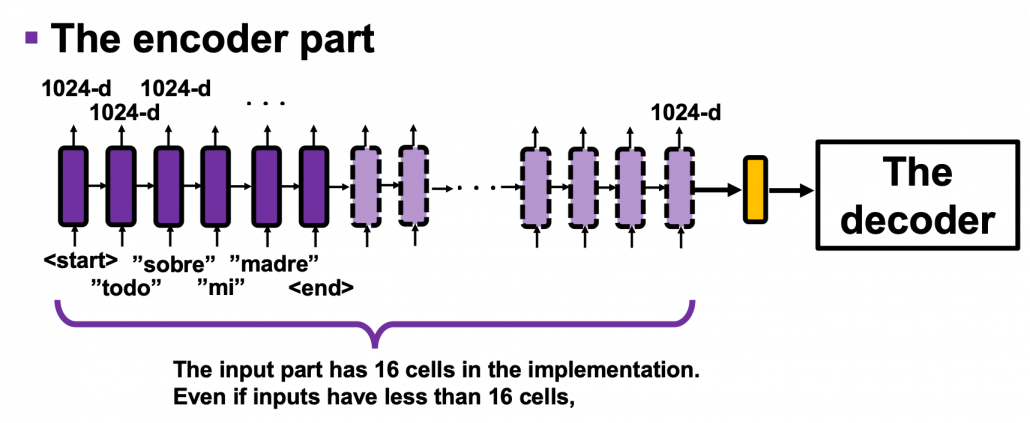
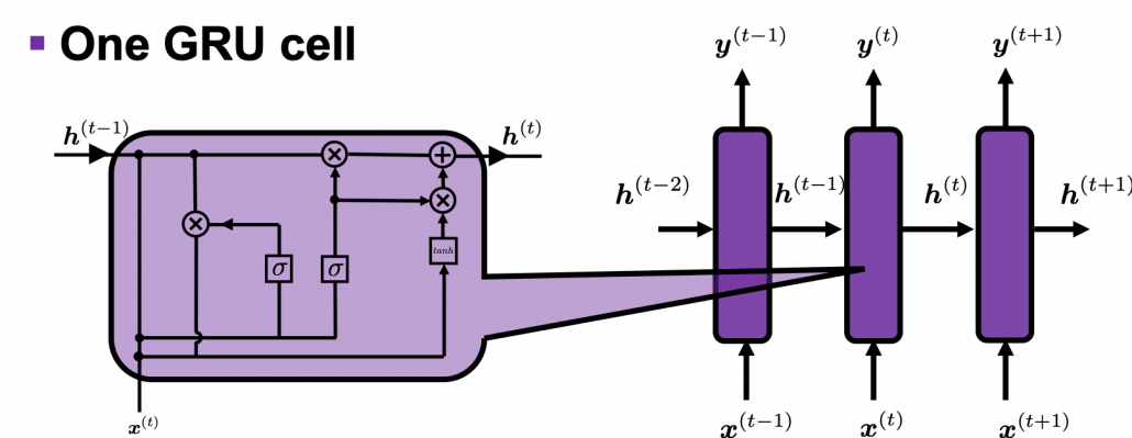
Let’s see how encoders are implemented in the code below. We use a type of RNN named GRU (Gated Recurrent Unit). GRU is simpler than LSTM (Long Short-Term Memory). One GRU cell gets an input every time step, and passes one hidden state via recurrent connections. As well as LSTM, GRU is a gated RNN so that it can mitigate vanishing gradient problems. GRU was invented after LSTM for smaller computation costs. At time step (t) one GRU cell gets an input \boldsymbol{x}^{(t)} and passes its hidden state/vector \boldsymbol{h}^{(t)} to the next cell like the figure below. But in the implementation, you put the whole input sentence as a 16 dimensional vector whose elements are integers, as you saw in the figure in the last subsection 2.1. That means, the ‘Encoder’ class in the implementation below makes a chain of 16 GRU cells every time you put an input sentence in Spanish, even if input sentences have less than 16 tokens.

*TO BE  VERY HONEST, I am not sure why the encoder part of  seq2seq models are implemented this way in the codes below. In the implementation below, the number of total time steps in the encoder part is fixed to 16. If input sentences have less than 16 tokens, it seems the RNN cells get no inputs after the time step of the token “<end>”. As far as I could check, if RNN cells get no inputs, they repeats giving out similar 1024-d vectors. I think in this implementation, RNN cells after the <end> token, which I showed as the dotted RNN cells in the figure above, do not change so much. And the encoder part passes the hidden state of the 16th RNN cell, which is in yellow, to the decoder.

2.3 The decoder

The decoder part is also not that hard to understand. As I briefly explained in the last section, you initialize the first cell of the decoder, using the hidden layer of the last cell the encoder. During decoding, I mean while writing a translation, at the beginning you put the token “<start>” as the first input of the decoder. Given the input “<start>”, the first cell outputs “all” in the example in the figure below, and the output “all” is the input of the next cell. The output of the next cell “about” is also passed to the next cell, and you repeat this till the decoder gives out the token “<end>”.

A more important point is how to get losses in the decoder part during training. We use a technique named teacher enforcing during training the decoder part of a seq2seq model. This is also quite simple: you just have to make sure you input a correct answer to RNN cells, regardless of the outputs generated by the cell last time step. You force the decoder to get the correct input every time step, and that is what teacher forcing is all about.

You can see how the decoder part and teacher forcing is implemented in the codes below. You have to keep it in mind that unlike the ‘Encoder’ class, you put a token into a ‘Decoder’ class every time step. To be exact you also need the outputs of the encoder part to calculate attentions in the decoder part. I am going to explain that in the next subsection.

2.4 Attention mechanism

I think you have learned at least one foreign language, and usually you have to translate some sentences. Remember the processes of writing a translation of a sentence in another language. Imagine that you are about to write a new word after writing some. If you are not used to translations in the language, you must have cared about which parts of the original language correspond to the very new word you are going to write. You have to pay “attention” to the original sentence. This is what attention mechanism is all about.

*I would like you to pay “attention” to this section. As you can see from the fact that the original paper on Transformer model is named “Attention Is All You Need,” attention mechanism is a crucial idea of Transformer.

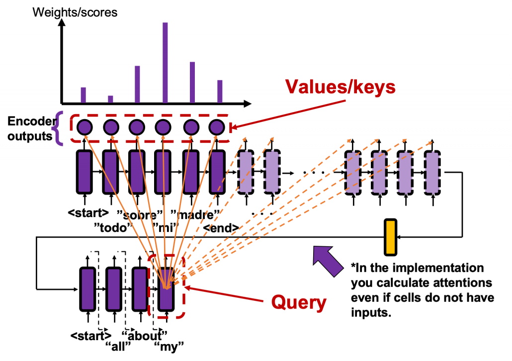
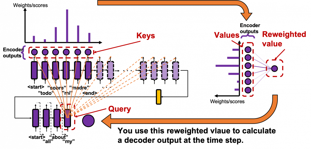
In the decoder part you initialize the hidden layer with the last hidden layer of the encoder, and its first input is “<start>”.  The decoder part start decoding, , as I explained in the last subsection. If you use attention mechanism in the seq2seq model, you calculate attentions every times step.  Let’s consider an example in the figure below, where the next input in the decoder is “my”, and given the token “my”, the GRU cell calculates a hidden state at the time step. The hidden state is the “query” in this case, and you compare the “query” with the 6 outputs of the encoder, which are “keys”. You get weights/scores, I mean “attentions”, which is the histogram in the figure below.

And you reweight the “values” with the weights in the histogram. In this case the “values” are the outputs of the encoder themselves. You used use the reweighted “values” to calculate the hidden state of the decoder at the times step again. And you used the hidden state updated by the attentions to predict the next word.

*In the implementation, however, the size of the output of the ‘Encoder’ class is always (16, 2024). You calculate attentions for all those 16 output vectors, but virtually only the first 6 1024-d output vectors important.

Summing up the points I have explained, you compare the “query” with the “keys” and get a scores/weights for the “values.” Each score/weight is in short relevance between the “query” and each “key”. And you reweight the “values” with the scores/weights.  In the case of attention mechanism in this article, we can say that “values” and “keys” are the same. You would also see that more clearly in the implementation below.

You especially have to pay attention to the terms “query”, “key”, and “value.” “Keys” and “values” are basically in the same language, and in the case above, they are in Spanish. “Queries” and “keys” can be in either different or the same. In the example above, the “query” is in English, and the “keys” are in Spanish.

You can compare a “query” with “keys” in various ways. The implementation uses the one called  Bahdanau’s additive style, and in Transformer, you use more straightforward ways. You do not have to care about how Bahdanau’s additive style calculates those attentions. It is much more important to learn the relations of “queries”, “keys”, and “values” for now.

*A problem is that Bahdanau’s additive style is slightly different from the figure above. It seems in Bahdanau’s additive style, at the time step (t) in the decoder part, the query is the hidden state at the time step (t-1). You would notice that if you closely look at the implementation below.As you can see in the figure above, you can see that you have to calculate the hidden state of the decoder cell two times at the time step (t): first in order to generate a “query”, second in order to predict the translated word at the time step. That would not be so computationally efficient, and I guess that is why Bahdanau’s additive style uses the hidden layer at the last time step as a query rather than calculating hidden layers twice.

2.5 Translating and displaying attentions

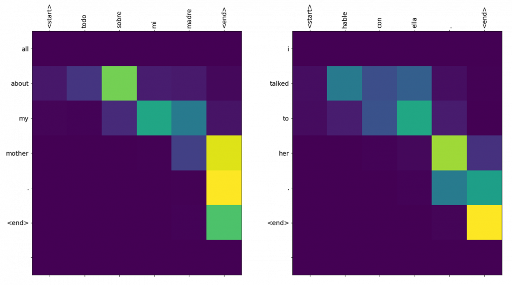
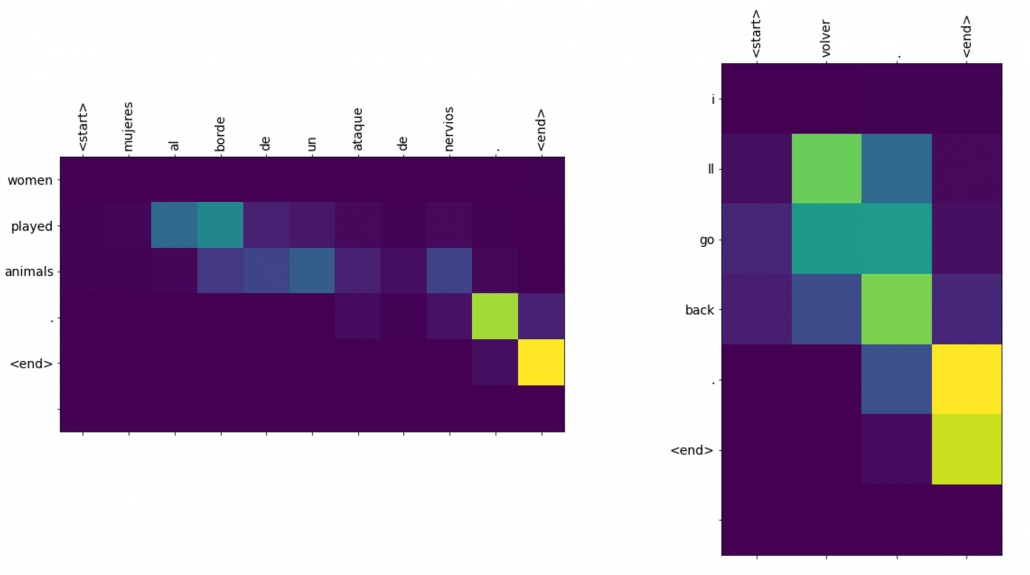
After training the translator for 20 epochs, I could translate Spanish sentences, and the implementation also displays attention scores for between the input and output sentences. For example the translation of the inputs “Todo sobre mi madre.” and “Habre con ella.” were “all about my mother .” and “i talked to her .” respectively, and the results seem fine. One powerful advantage of using attention mechanism is you can display this type of word alignment, I mean correspondences of words in a sentence, easily as in the heat maps below. The yellow parts shows high scores of attentions, and you can see that the distributions of relatively highs scores are more or less diagonal, which implies that English and Spanish have similar word orders.

For other inputs like “Mujeres al borde de un ataque de nervious.” or “Volver.”, the translations are not good.

You might have noticed there is one big problem in this implementation: you can use only the words appeared in the corpus. And actually I had to manually add some pairs of sentences with the word “borde” to the corpus to get the translation in the figure.

* I make study materials on machine learning, sponsored by DATANOMIQ. I do my best to make my content as straightforward but as precise as possible. I include all of my reference sources. If you notice any mistakes in my materials, including grammatical errors, please let me know (email: yasuto.tamura@datanomiq.de). And if you have any advice for making my materials more understandable to learners, I would appreciate hearing it.

How to Efficiently Manage Big Data

The benefits of big data today can’t be ignored, especially since these benefits encompass industries. Despite the misconceptions around big data, it has shown potential in helping organizations move forward and adapt to an ever-changing market, where those that can’t respond appropriately or quickly enough are left behind. Data analytics is the name of the game, and efficient data management is the main differentiator.

A digital integration hub (DIH) will provide the competitive edge an organization needs in the efficient handling of data. It’s an application architecture that aggregates operational data into a low-latency data fabric and helps in digital transformation by offloading from legacy architecture and providing a decoupled API layer that effectively supports modern online applications. Data management entails the governance, organization, and administration of large, and possibly complex, datasets. The rapid growth of data pooIs has left unprepared companies scrambling to find solutions that will help keep them above water. Data in these pools originate from a myriad of sources, including websites, social media sites, and system logs. The variety in data types and their sheer size make data management a fairly complex undertaking.

Big Data Management for Big Wins

In today’s data-driven world, the capability to efficiently analyze and store data are vital factors in enhancing current business processes and setting up new ones. Data has gone beyond the realm of data analysts and into the business mainstream. As such, businesses should add data analysis as a core competency to ensure that the entire organization is on the same page when it comes to data strategy. Below are a few ways you can make big data work for you and your business.

Define Specific Goals

The data you need to capture will depend on your business goals so it’s imperative that you know what these are and ensure that these are shared across the organization. Without definite and specific goals, you’ll end up with large pools of data and nowhere to use them in. As such, it’s advisable to involve the entire team in mapping out a data strategy based on the company’s objectives. This strategy should be part of the organization’s overall business strategy to avoid the collection of irrelevant data that has no impact on business performance. Setting the direction early on will help set you up for long-term success.

Secure Your Data

Because companies have to contend with large amounts of data each day, storage and management could become very challenging. Security is also a main concern; no organization wants to lose it’s precious data after spending time and money processing and storing them. While keeping data accessible for analysis, you should also ensure that it’s kept secure at all times. When handling data, you should have security measures in place, such as firewall security, malware scanning, and spam filtering. Data security is especially important when collecting customer data to avoid violating data privacy regulations. Ideally, it should be one of the main considerations in data management because it’s a critical factor that could mean the difference between a successful venture and a problematic one.

Interlink Your Data

Different channels can be used to access a database, but this doesn’t necessarily mean that you should use several or all of them. There’s no need to deploy different tools for each application your organization uses. One of the ways to prevent miscommunication between applications and ensure that data is synchronized at all times is to keep data interlinked. Synchronicity of data is vital if your organization or team plans to use a single database. An in-memory data grid, cloud storage system, and remote database administrator are just some of the tools a company can use to interlink data.

Ensure Compliance With Audit Regulations

One thing that could be easy to overlook is how compliant systems are to audit regulations. A database and it is conducted to check on the actions of database users and managers. It is typically done for security purposes—to ensure that data or information can be accessed only by those authorized to do so. Adhering to audit regulations is a must, even for offsite database administrators, so it’s critical that they maintain compliant database components.

Be Prepared for Change

There have been significant changes in the field of data processing and management in recent years, which indicates a promising yet constantly changing landscape. To get ahead of the data analytics game, it’s vital that you keep up with current data trends. New tools and technology are made available at an almost regular pace, and keeping abreast of them will ensure that a business keeps its database up to date. It’s also important to be flexible and be able to pivot or restrategize at a moment’s notice so the business can adapt to change accordingly.

Big Data for the Long Haul

Traditional data warehouses and relational database platforms are slowly becoming things of the past. Big data analytics has changed the game, with data management moving away from being a complex, IT-team focused function and becoming a core competency of every business. Ensuring efficient data management means giving your business a competitive edge, and implementing the tips above ensures that a business manages its data effectively. Changes in data strategies are certain, and they may come sooner than later. Equipping your people with the appropriate skills and knowledge will ensure that your business can embrace change with ease.

Data Mining Process flow – Easy Understanding

1 Overview

Development of computer processing power, network and automated software completely change and give new concept of each business. And data mining play the vital part to solve, finding the hidden patterns and relationship from large dataset with business by using sophisticated data analysis tools like methodology, method, process flow etc.

On this paper, proposed a process flow followed CRISP-DM methodology and has six steps where data understanding does not considered.

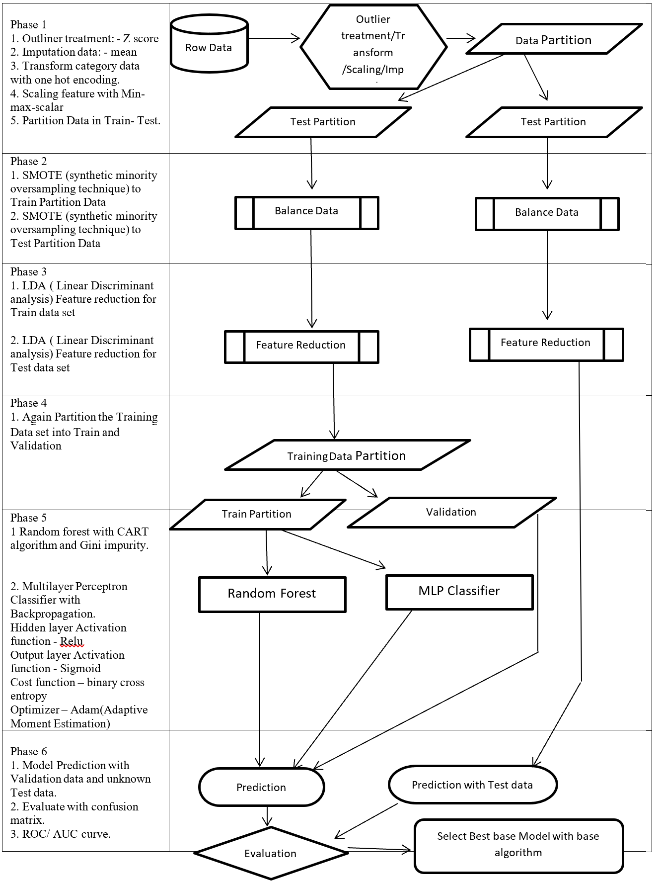
Phase of new process flow given below:-

Phase 1: Involved with collection, outliner treatment, imputation, transformation, scaling, and partition dataset in to two sub-frames (Training and Testing). Here as an example for outliner treatment, imputation, transformation, scaling consider accordingly Z score, mean, One hot encoding and Min Max Scaler.

Phase 2: On this Phase training and testing data balance with same balancing algorithm but separately. As an example here SMOTE (synthetic minority oversampling technique) is considered.

Phase 3: This phase involved with reduction, selection, aggregation, extraction. But here for an example considering same feature reduction algorithm (LDA -Linear Discriminant analysis) on training and testing data set separately.

Phase 4: On this Phase Training data set again partition into two more set (Training and Validation).

Phase 5: This Phase considering several base algorithms as a base model like CNN, RNN, Random forest, MLP, Regression, Ensemble method. This phase also involve to find out best hyper parameter and sub-algorithm for each base algorithm. As an example on this paper consider two class classification problems and also consider Random forest (Included CART – Classification and Regression Tree and GINI index impurity) and MLP classifier (Included (Relu, Sigmoid, binary cross entropy, Adam – Adaptive Moment Estimation) as base algorithms.

Phase 6: First, Prediction with validation data then evaluates with Test dataset which is fully unknown for these (Random forest, MLP classifier) two base algorithms. Then calculate the confusion matrix, ROC, AUC to find the best base algorithm.

New method from phase 1 to phase 4 followed CRISP-DM methodology steps such as data collection, data preparation then phase 5 followed modelling and phase 6 followed evaluation and implementation steps.

Structure of proposed process flow for two class problem combined with algorithm and sub-algorithm display on figure – 1.

These articles mainly focus to describe all algorithms which are going to implementation for better understanding.


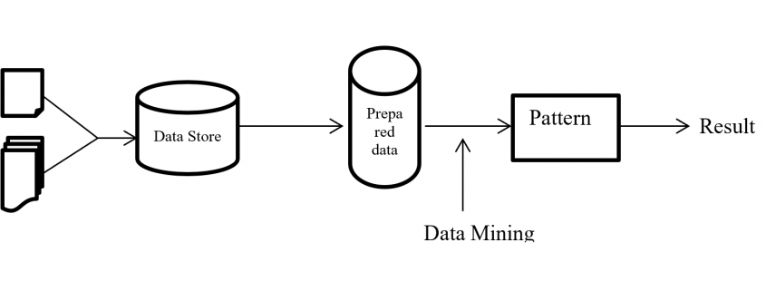
Data Mining Process Flow

Figure 1 – Data Mining Process Flow

2 Phase 1: Outlier treatment, Transform, Scaling, Imputation

This phase involved with outlier treatment, imputation, scaling, and transform data.

2.1 Outliner treatment: – Z score

Outlier is a data point which lies far from all other data point in a data set. Outlier need to treat because it may bias the entire result. Outlier treatment with Z score is a common technique.  Z score is a standard score in statistics.  Z score provides information about data value is smaller or grater then mean that means how many standard deviations away from the mean value. Z score equation display below:

Z = \frac{(x - \mu)}{\sigma}

Here x = data point
σ = Standard deviation
μ = mean value

Equation- 1 Z-Score

In a normal distribution Z score represent 68% data lies on +/- 1, 95% data point lies on +/- 2, 99.7% data point lies on +/- 3 standard deviation.

2.2 Imputation data: – mean

Imputation is a way to handle missing data by replacing substituted value. There are many imputation technique represent like mean, median, mode, k-nearest neighbours. Mean imputation is the technique to replacing missing information with mean value. On the mean imputation first calculate the particular features mean value and then replace the missing value with mean value. The next equation displays the mean calculation:

\mu = \frac{(\sum x)}{n}

Here x = value of each point
n = number of values
μ = mean value

Equation- 2 Mean

2.3 Transform: – One hot encoding

Encoding is a pre-processing technique which represents data in such a way that computer can understand.  For understanding of machine learning algorithm categorical columns convert to numerical columns, this process called categorical encoding. There are multiple way to handle categorical variable but most widely used techniques are label encoding and one host encoding. On label encoding give a numeric (integer number) for each category. Suppose there are 3 categories of foods like apples, orange, banana. When label encoding is used then 3 categories will get a numerical value like apples = 1, banana = 2 and orange = 3. But there is very high probability that machine learning model can capture the relationship in between categories such as apple < banana < orange or calculate average across categories like 1 +3 = 4 / 2 = 2 that means model can understand average of apple and orange together is banana which is not acceptable because model correlation calculation is wrong. For solving this problem one hot encoding appear. The following table displays the label encoding is transformed into one hot encoding.

Label Encoding and One-Hot-Encoding

Table- 1 Encoding example

On hot encoding categorical value split into columns and each column contains 0 or 1 according to columns placement.

2.4 Scaling data: – Min Max Scaler

Feature scaling method is standardized or normalization the independent variable that means it is used to scale the data in a particular range like -1 to +1 or depending on algorithm. Generally normalization used where data distribution does not follow Gaussian distribution and standardization used where data distribution follow Gaussian distribution. On standardization techniques transform data values are cantered around the mean and unit is standard deviation. Formula for standardization given below:

Standardization X = \frac{(X - \mu)}{\sigma}

Equation-3 Equations for Standardization

X represent the feature value, µ represent mean of the feature value and σ represent standard deviation of the feature value. Standardized data value does not restrict to a particular range.

Normalization techniques shifted and rescaled data value range between 0 and 1. Normalization techniques also called Min-Max scaling. Formula for normalization given below:

Normalization X = \frac{(X - X_{min})}{X_{max} - X_{min}}

Equation – 4 Equations for Normalization

Above X, Xmin, Xmax are accordingly feature values, feature minimum value and feature maximum value. On above formula when X is minimums then numerator will be 0 (  is 0) or if X is maximums then the numerator is equal to the denominator (  is 1). But when X data value between minimum and maximum then  is between 0 and 1. If ranges value of data does not normalized then bigger range can influence the result.

3 Phase 2: – Balance Data

3.1 SMOTE

SMOTE (synthetic minority oversampling technique) is an oversampling technique where synthetic observations are created based on existing minority observations. This technique operates in feature space instead of data space. Under SMOTE each minority class observation calculates k nearest neighbours and randomly chose the neighbours depending on over-sampling requirements. Suppose there are 4 data point on minority class and 10 data point on majority class. For this imbalance data set, balance by increasing minority class with synthetic data point.   SMOTE creating synthetic data point but it is necessary to consider k nearest neighbours first. If k = 3 then SMOTE consider 3 nearest neighbours. Figure-2 display SMOTE with k = 3 and x = x1, x2, x3, x4 data point denote minority class. And all circles represent majority class.
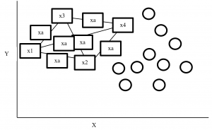
SMOTE Example

Figure- 2 SMOTE example


4 Phase 3: – Feature Reduction

4.1 LDA

LDA stands for Linear Discriminant analysis supervised technique are commonly used for classification problem.  On this feature reduction account continuous independent variable and output categorical variable. It is multivariate analysis technique. LDA analyse by comparing mean of the variables.  Main goal of LDA is differentiate classes in low dimension space. LDA is similar to PCA (Principal component analysis) but in addition LDA maximize the separation between multiple classes. LDA is a dimensionality reduction technique where creating synthetic feature from linear combination of original data set then discard less important feature. LDA calculate class variance, it maximize between class variance and minimize within class variance. Table-2 display the process steps of LDA.

LDA Process

Table- 2 LDA process

5 Phase 5: – Base Model

Here we consider two base model ensemble random forest and MLP classifier.

5.1 Random Forest

Random forest is an ensemble (Bagging) method where group of weak learner (decision tree) come together to form a strong leaner. Random forest is a supervised algorithm which is used for regression and classification problem. Random forests create several decisions tree for predictions and provide solution by voting (classification) or mean (regression) value. Working process of Random forest given below (Table -3).

Random Forest

Table-3 Random Forest process

When training a Random forest root node contains a sample of bootstrap dataset and the feature is as same as original dataset. Suppose the dataset is D and contain d record and m number of columns. From the dataset D random forest first randomly select sample of rows (d) with replacement and sample of features (n) and give it to the decision tree. Suppose Random forest created several decision trees like T1, T2, T3, T4 . . . Tn. Then randomly selected dataset D = d + n is given to the decision tree T1, T2, T3, T4 . . . Tn where D < D, m > n and d > d.  After taking the dataset decision tree give the prediction for binary classification 1 or 0 then aggregating the decision and select the majority voted result. Figure-3 describes the structure of random forest process.
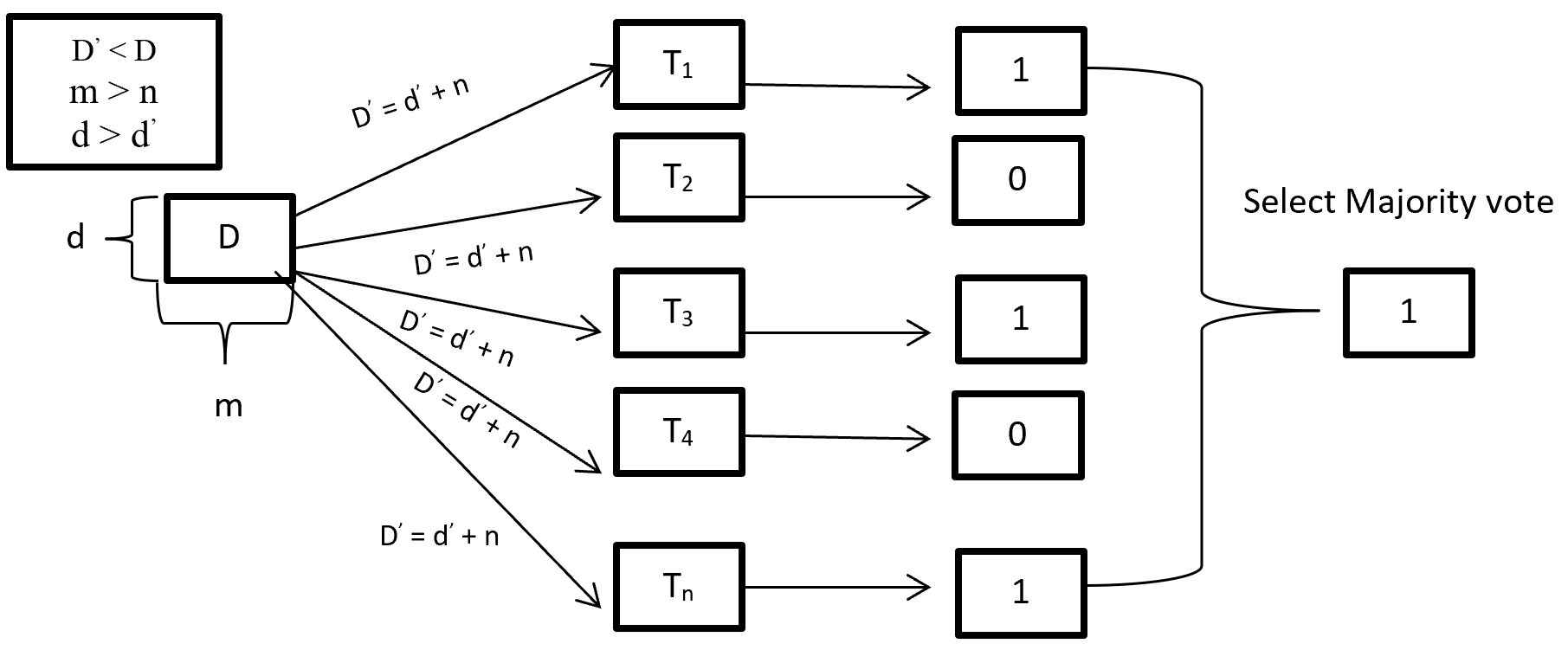
Random Forest Process

Figure- 3 Random Forest process

On Random forest base learner Decision Tree grows complete depth where bias (properly train on training dataset) is low and variance is high (when implementing test data give big error) called overfitting. On Random forest using multiple decision trees where each Decision tree is high variance but when combining all decision trees with the respect of majority vote then high variance converted into low variance because using row and feature sampling with replacement and taking the majority vote where decision is not depend on one decision tree.

CART (Classification and Regression Tree) is binary segmentation technique. CART is a Gini’s impurity index based classical algorithm to split a dataset and build a decision tree. By splitting a selected dataset CART created two child nodes repeatedly and builds a tree until the data no longer be split. There are three steps CART algorithm follow:

  1. Find best split for each features. For each feature in binary split make two groups of the ordered classes. That means possibility of split for k classes is k-1. Find which split is maximized and contain best splits (one for each feature) result.
  2. Find the best split for nodes. From step 1 find the best one split (from all features) which maximized the splitting criterion.
  3. Split the best node from step 2 and repeat from step 1 until fulfil the stopping criterion.


For splitting criteria CART use GINI index impurity algorithm to calculate the purity of split in a decision tree. Gini impurity randomly classified the labels with the same distribution in the dataset. A Gini impurity of 0 (lowest) is the best possible impurity and it is achieve when everything is in a same class. Gini index varies from 0 to 1. 0 indicate the purity of class where only one class exits or all element under a specific class. 1 indicates that elements are randomly distributed across various classes. And 0.5 indicate equal elements distributed over classes. Gini index (GI) described by mathematically that sum of squared of probabilities of each class (pi) deducted from one (Equation-5).

Gini Impurities

Equation – 5 Gini impurities

Here (Equation-5) pi represent the probability (probability of p+ or yes and probability of p- or no) of distinct class with classified element. Suppose randomly selected feature (a1) which has 8 yes and 4 no. After the split right had side (b1 on equation-6) has 4 yes and 4 no and left had side (b2 on equation – 7) has 4 yes and 0 no. here b2 is a pure split (leaf node) because only one class yes is present. By using the GI (Gini index) formula for b1 and b2:-
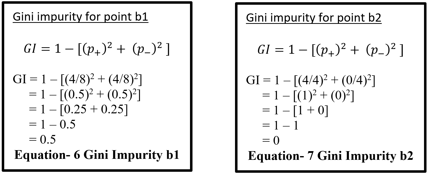
Equation- 6 & 7 – Gini Impurity b1 & Gini Impurity b2

Here for b1 value 0.5 indicates that equal element (yes and no) distribute over classes which is not pure split. And b2 value 0 indicates pure split. On GINI impurity indicates that when probability (yes or no) increases GINI value also increases. Here 0 indicate pure split and .5 indicate equal split that means worst situation. After calculating the GINI index for b1 and b2 now calculate the reduction of impurity for data point a1. Here total yes 8 (b1 and b2 on Equation – 8) and total no 4 (b1) so total data is 12 on a1. Below display the weighted GINI index for feature a1:

Total data point on b1 with Gini index (m) = 8/12 * 0.5 = 0.3333

Total data point on b2 with Gini index (n) = 4/12 * 0 = 0

Weighted Gini index for feature a1 = m + n = 0.3333

Equation- 8 Gini Impurity b1 & b2

After computing the weighted Gini value for every feature on a dataset taking the highest value feature as first node and split accordingly in a decision tree. Gini is less costly to compute.

5.2 Multilayer Perceptron Classifier (MLP Classifier)

Multilayer perceptron classifier is a feedforward neural network utilizes supervised learning technique (backpropagation) for training. MLP Classifier combines with multiple perceptron (hidden) layers. For feedforward taking input send combining with weight bias and then activation function from one hidden layer output goes to other hidden and this process continuing until reached the output. Then output calculates the error with error algorithm. These errors send back with backpropagation for weight adjustment by decreasing the total error and process is repeated, this process is call epoch. Number of epoch is determined with the hyper-parameter and reduction rate of total error.

5.2.1 Back-Propagation

Backpropagation is supervised learning algorithm that is used to train neural network. A neural network consists of input layer, hidden layer and output layer and each layer consists of neuron. So a neural network is a circuit of neurons. Backpropagation is a method to train multilayer neural network the updating of the weights of neural network and is done in such a way so that the error observed can be reduced here, error is only observed in the output layer and that error is back propagated to the previous layers and previous layer is proportionally updated weight. Backpropagation maintain chain rule to update weight. Mainly three steps on backpropagation are (Table-4):

Step Process
Step 1 Forward Pass
Step 2 Backward Pass
Step 3 Sum of all values and calculate updated weight value with Chain – rules.

Table-4 Back-Propagation process

5.2.2 Forward pass/ Forward propagation

Forward propagation is the process where input layer send the input value with randomly selected weight and bias to connected neuron and inside neuron selected activation function combine them and forward to other connected neuron layer after layer then give an output with the help of output layer. Below (Figure-4) display the forward propagation.
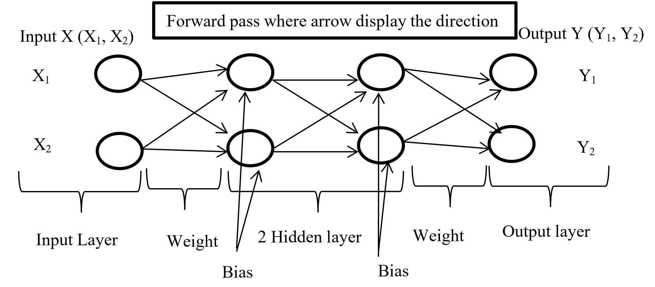
Foreward Pass

Figure-4 Forward passes

Input layer take the input of X (X1, X2) combine with randomly selected weight for each connection and with fixed bias (different hidden layer has different bias) send it to first hidden layer where first multiply the input with corresponding weight and added all input with single bias then selected activation function (may different form other layer) combine all input and give output according to function and this process is going on until reach in output layer. Output layer give the output like Y (Y1, Y2) (here output is binary classification as an example) according to selected activation function.

5.2.3 Backward Pass

After calculating error (difference between Forward pass output and actual output) backward pass try to minimize the error with optimisation function by sending backward with proportionally distribution and maintain a chain rule. Backward pass distribution the error in such a way where weighted value is taking under consideration. Below (Figure-5) diagram display the Backward pass process.
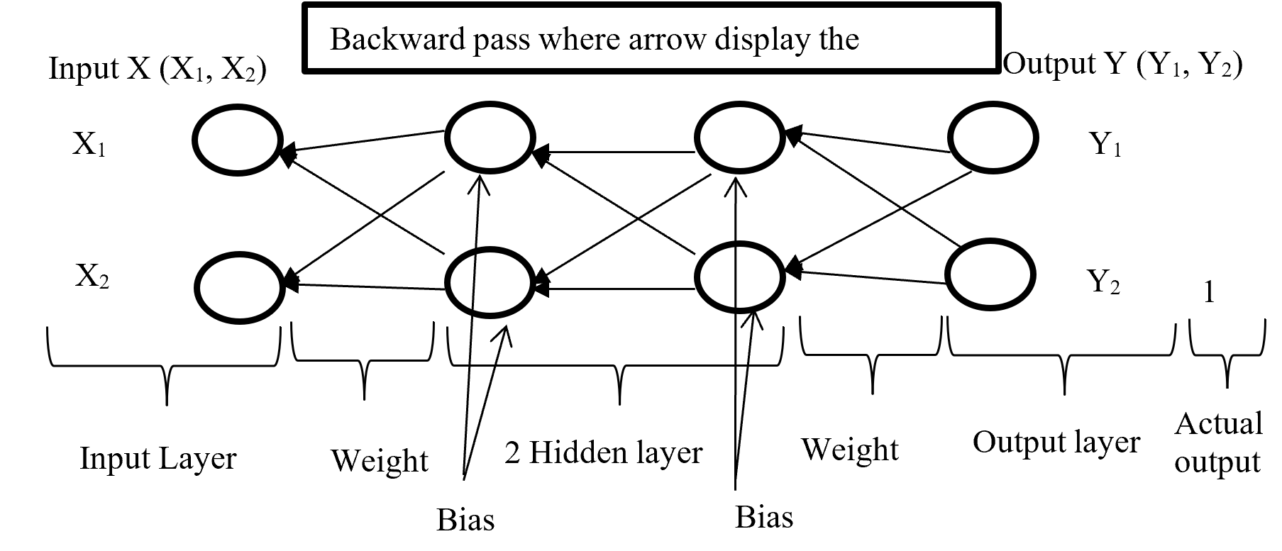
Backward Pass

Figure-5 Backward passes

Backpropagation push back the error which is calculated with error function or loss function for update proportional distribution with the help of optimisation algorithm. Division of Optimisation algorithm given below on Figure – 6
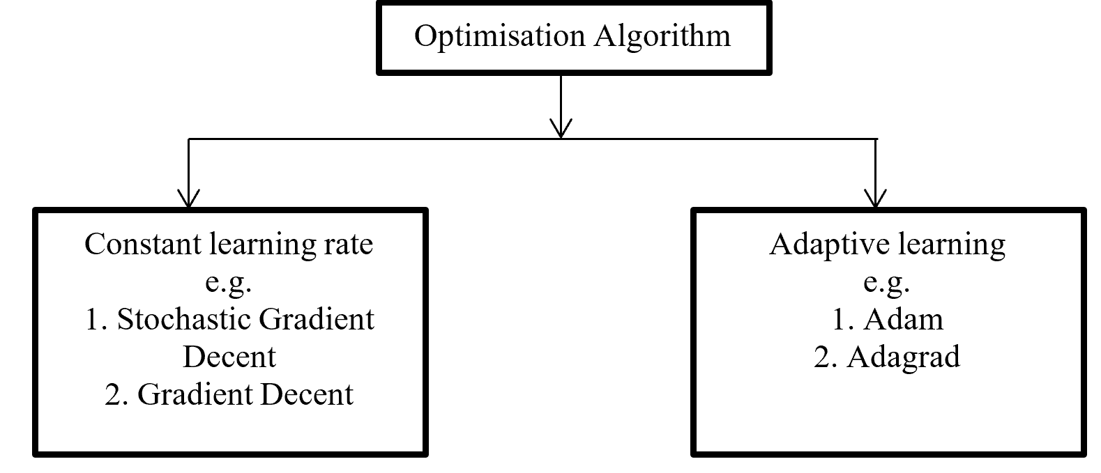
Optimisation Algorithms

Figure -6 Division of Optimisation algorithms

Gradient decent calculate gradient and update value by increases or decreases opposite direction of gradients unit and try to find the minimal value. Gradient decent update just one time for whole dataset but stochastic gradient decent update on each training sample and it is faster than normal gradient decent. Gradient decent can be improve by tuning parameter like learning rate (0 to 1 mostly use 0.5). Adagrad use time step based parameter to compute learning rate for every parameter. Adam is Adaptive Moment Estimation. It calculates different parameter with different learning rate. It is faster and performance rate is higher than other optimization algorithm. On the other way Adam algorithm is squares the calculated exponential weighted moving average of gradient.

5.2.4 Chain – rules

Backpropagation maintain chain-rules to update weighted value. On chain-rules backpropagation find the derivative of error respect to any weight. Suppose E is output error. w is weight for input a and bias b and ac neuron output respect of activation function and summation of bias with weighted input (w*a) input to neuron is net. So partial derivative for error respect to weight is ∂E / ∂w display the process on figure-7.

Figure- 7 Partial derivative for error respect to weight

On the chain rules for backward pass to find (error respect to weight) ∂E / ∂w = ∂E / ∂ac * ∂ac / ∂net * ∂net / ∂w. here find to error respect to weight are error respect to output of activation function multiply by activation function output respect to input in a neuron multiply by input in a neuron respect to weight.

5.2.5 Activation function

Activation function is a function which takes the decision about neuron to activate or deactivate. If the activate function activate the neuron then it will give an output on the basis of input. Input in a activation function is sum of input multiply with corresponding weight and adding the layered bias.  The main function of a activate function is non-linearity output of a neuron.
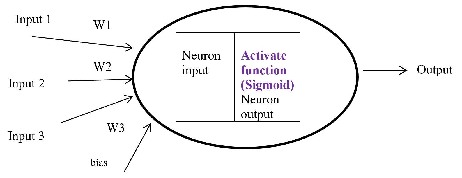
Activation Function

Figure-8 Activation function

Figure – 8 display a neuron in a hidden layer. Here several input (1, 2, 3) with corresponding weight (w1, w2, w3) putting in a neuron input layer where layer bias add with summation of multiplication with input and weight. Equation-9 display the output of an activate function.

Output from activate function y = Activate function (Ʃ (weight * input) + bias)

y = f (Ʃ (w*x) +b)

Equation- 9 Activate function

There are many activation functions like linear function for regression problem, sigmoid function for binary classification problem where result either 0 or 1, Tanh function which is based on sigmoid function but mathematically shifted version and values line -1 to 1. RELU function is Rectified linear unit. RELU is less expensive to compute.

5.2.6 Sigmoid

Sigmoid is a squashing activate function where output range between 0 and 1. Sigmoidal name comes from Greek letter sigma which looks like letter S when graphed. Sigmoid function is a logistic type function, it mainly use in output layer in neural network. Sigmoid is non-linear, fixed output range (between 0 and 1), monotonic (never decrees or never increases) and continuously differentiated function. Sigmoid function is good at classification and output from sigmoid is nonlinear. But Sigmoid has a vanishing gradient problem because output variable is very less to change in input variable. Figure- 9 displays the output of a Sigmoid and derivative of Sigmoid. Here x is any number (positive or negative). On sigmoid function 1 is divided by exponential negative input with adding 1.
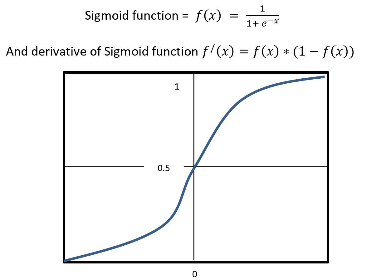
Sigmoid

Figure – 9 Sigmoid Functions

4.5.2.7 RELU

RELU stands for Rectified Linear Units it is simple, less expensive in computation and rectifies the gradient vanishing problem. RELU is nonlinear activation function. It gives output either positive (infinity) or 0. RELU has a dying problem because if neurons stop for responding to variation because of gradient is 0 or nothing has to change. Figure- 10 displays the output of an RELU and derivative of RELU. Here x is any positive input and if x is grater then 0 give the output as x or give output 0. RELU function gives the output maximum value of input, here max (0, x).
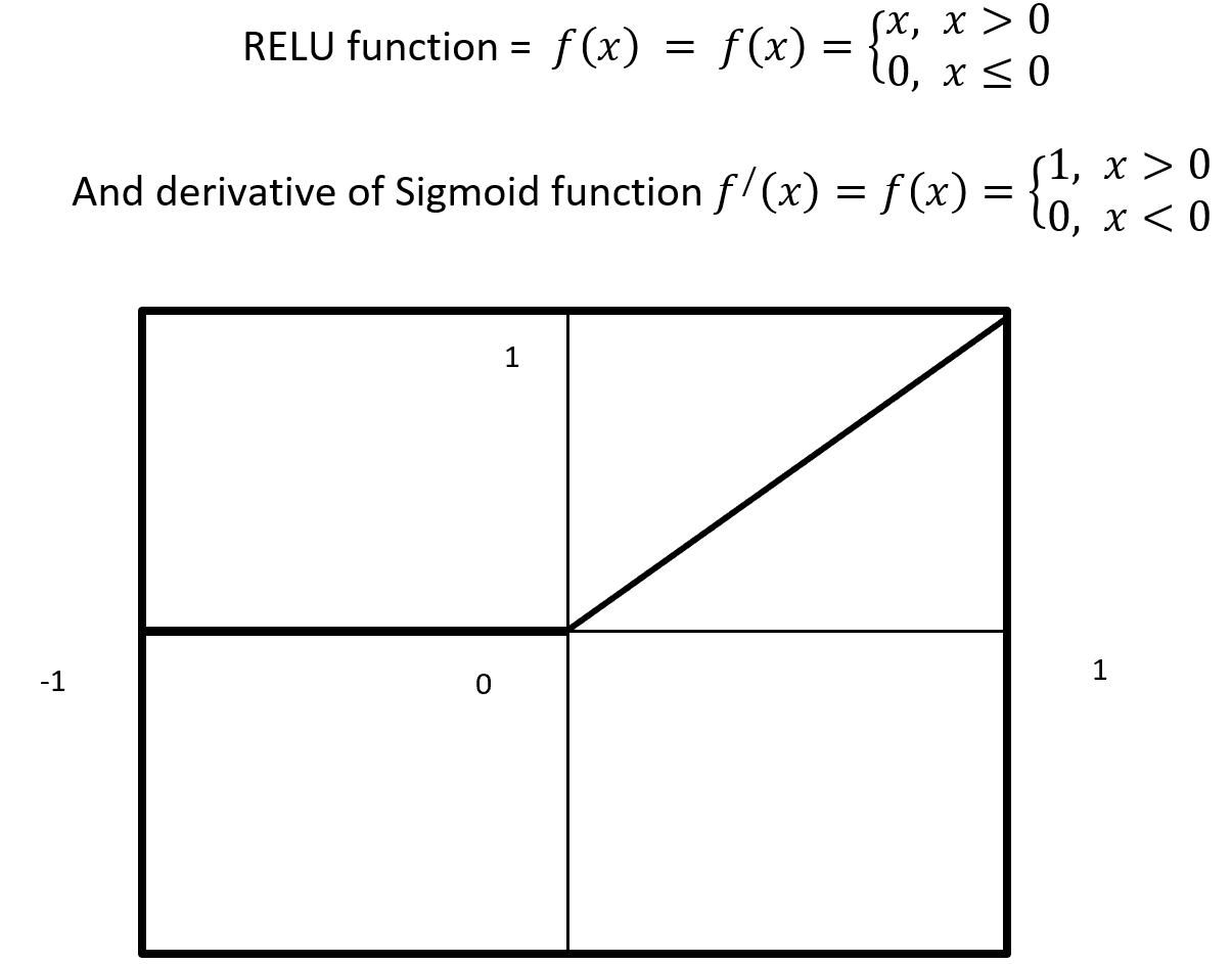
Relu Activation Function

Figure – 10 RELU Function

4.5.2.8 Cost / loss function (Binary Cross-Entropy)

Cost or loss function compare the predictive value (model outcome) with actual value and give a quantitative value which give the indication about how much good or bad the prediction is.
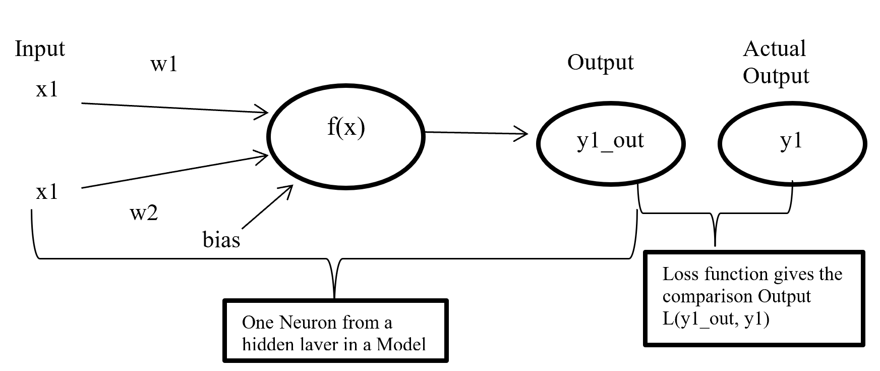
Cost Function

Figure- 11 Cost function work process

Figure-11 x1 and x2 are input in a activate function f(x) and output y1_out which is sum of weighted input added with bias going through activate function. After model output activate function compare the output with actual output and give a quantitative value which indicate how good or bad the prediction is.

There are many type of loss function but choosing of optimal loss function depends on the problem going to be solved such as regression or classification. For binary classification problem binary cross entropy is used to calculate cost. Equation-10 displays the binary cross entropy where y is actual binary value and yp predictive outcome range 0 and 1. And i is scalar vale range between 1 to model output size (N).

Binary Crossentropy

Equation-10 displays the binary cross entropy

6 Phase 6: – Evaluation

6.1 Confusion matrix

In a classification confusion matrix describe the performance of actual value against predictive value. Confusion Matrix does the performance measurement. So confusion matrix classifies and display predicted and actual value (Visa, S., Ramsay 2011).
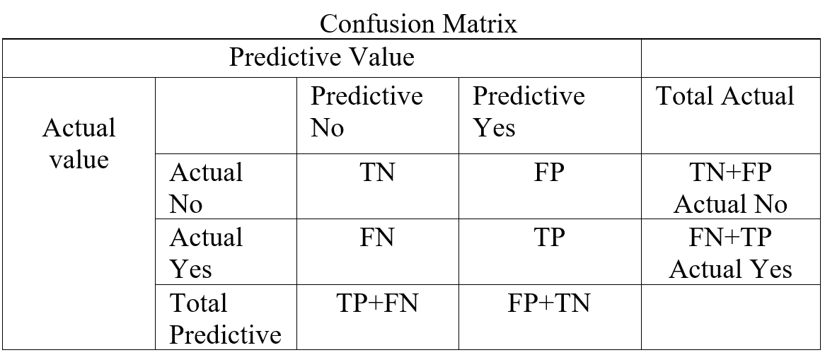
Confusion Matrix

Table- 5 Confusion Matrix

Confusion Matrix (Table-5) combines with True Positive (TP), True Negative (TN), False Positive (FP), and False Negative (FN). True Positive is prediction positive and true. True Negative is prediction negative and that is true. False positive is prediction positive and it’s false. False negative is prediction negative and that is false. False positive is known as Type1 error and false negative is known as Type 2 error. Confusion matrix can able to calculate several list of rates which are given below on Table- 6.

Here    N = Total number of observation, TP = True Positive, TN = True Negative

FP = False Positive, FN = False Negative, Total Actual No (AN) = TN + FP,

Total Predictive Yes (PY) = FP + TP. Total Actual Yes (AY) = FN + TP

Rate


Description Mathematical Description
Accuracy Classifier, overall how often correctly identified  (TP+TN) / N
Misclassification Rate Classifier, overall how often wrongly identified (FP + FN) / N
True Positive Rate

(Sensitivity / Recall)

Classifier, how often predict correctly yes when it is actually yes.  TP / AY
False Positive Rate Classifier, how often predict wrongly yes when it is actually no.  FP / AN
True Negative Rate

(Specificity)

Classifier, how often predict correctly no when it is actually no.  TN / AN
Precision Classifier how often predict yes when it is correct.  TP / PY
Prevalence Yes conditions how often occur in a sample. AY / N

Table – 6 Confusion matrixes Calculation

From confusion matrix F1 score can be calculated because F1 score related to precision and recall. Higher F1 score is better. If precision or recall any one goes down F1 score also go down.

F1 = \frac{2 * Precision * Recall}{Precision + Recall}

4.6.2 ROC (Receiver Operating Characteristic) curve

In statistics ROC is represent in a graph with plotting a curve which describe a binary classifiers performance as its differentiation threshold is varied. ROC (Equation-11) curve created true positive rate (TPR) against false positive rate (FPR). True positive rate also called as Sensitivity and False positive rate also known as Probability of false alarm. False positive rate also called as a probability of false alarm and it is calculated as 1 – Specificity.

True Positive Rate = \frac{True Positive}{True Positive + False Negative} = Recall or Sensivity

False Positive Rate = \frac{True Negative}{True Negative + False Positive} = 1 - Specificity

Equation- 11 ROC

So ROC (Receiver Operation Characteristic) curve allows visual representation between sensitivity and specificity associated with different values of the test result (Grzybowski, M. and Younger, J.G., 1997)

On ROC curve each point has different Threshold level. Below (Figure – 12) display the ROC curve. Higher the area curve covers is better that means high sensitivity and high specificity represent more accuracy. ROC curve also represent that if classifier predict more often true than it has more true positive and also more false positive. If classifier predict true less often then fewer false positive and also fewer true positive.
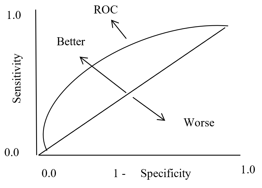
ROC Curve

ROC Curve

Figure – 12 ROC curve description

4.6.3 AUC (Area under Curve)

Area under curve (AUC) is the area surrounded by the ROC curve and AUC also represent the degree of separability that means how good the model to distinguished between classes. Higher the AUC value represents better the model performance to separate classes. AUC = 1 for perfect classifier, AUC = 0 represent worst classifier, and AUC = 0.5 means has no class separation capacity. Suppose AUC value is 0.6 that means 60% chance that model can classify positive and negative class.

Figure- 13 to Figure – 16 displays an example of AUC where green distribution curve for positive class and blue distribution curve for negative class. Here threshold or cut-off value is 0.5 and range between ‘0’ to ‘1’. True negative = TN, True Positive = TP, False Negative = FN, False Positive = FP, True positive rate = TPR (range 0 to 1), False positive rate = FPR (range 0 to 1).

On Figure – 13 left distribution curve where two class curves does not overlap that means both class are perfectly distinguished. So this is ideal position and AUC value is 1.  On the left side ROC also display that TPR for positive class is 100% occupied.
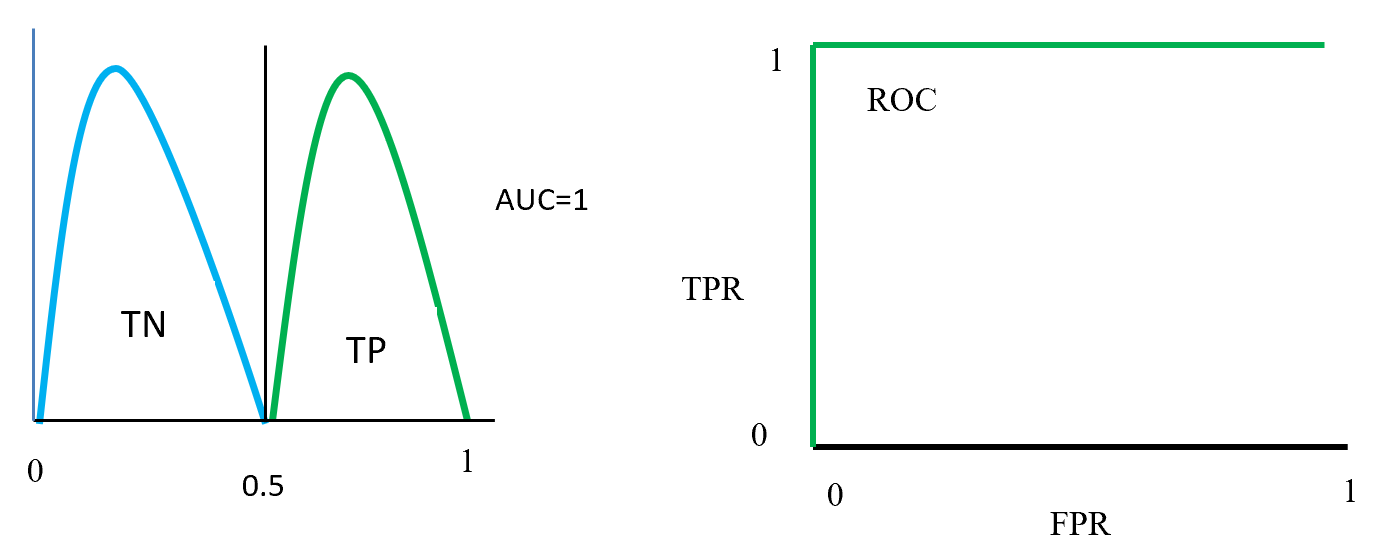
ROC distributions (perfectly distinguished

ROC distributions (perfectly distinguished

Figure – 14 two class overlap each other and raise false positive (Type 1), false negative (Type 2) errors. Here error could be minimize or maximize according to threshold. Suppose here AUC = 0.6, that means chance of a model to distinguish two classes is 60%. On ROC curve also display the curve occupied for positive class is 60%.

ROC distributions (class partly overlap distinguished)

ROC distributions (class partly overlap distinguished)

Figure- 15 displayed that positive and negative overlap each other. Here AUC value is 0.5 or near to 0.5. On this position classifier model does not able distinguish positive and negative classes. On left side ROC curve become straight that means TPR and FPR are equal.
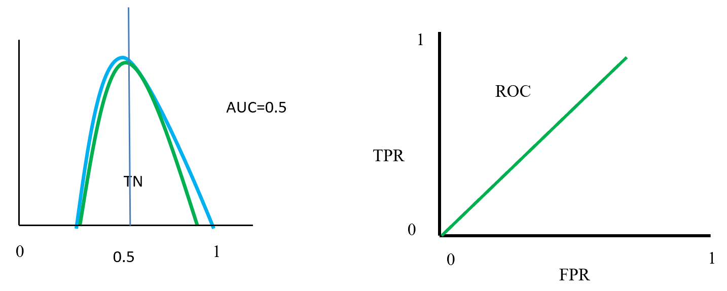
ROC distributions (class fully overlap distinguished)

ROC distributions (class fully overlap distinguished)

Figure- 16 positive and negative class swap position and on this position AUC = 0. That means classified model predict positive as a negative and negative as a positive. On the left ROC curve display that curve on FPR side fully fitted.
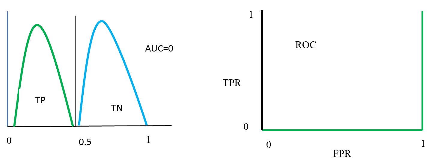
ROC distributions (class swap position distinguished)

ROC distributions (class swap position distinguished)

7 Summaries

This paper describes a data mining process flow and related model and its algorithm with textual representation. One hot encoding create dummy variable for class features and min-max scaling scale the data in a single format. Balancing by SMOTE data where Euclidian distance calculates the distance in-between nearest neighbour to produce synthetic data under minority class. LDA reduce the distance inside class and maximise distance in-between class and for two class problem give a single dimension features which is less costly to calculate accuracy by base algorithm (random forest and MLP classifier).  Confusion matrix gives the accuracy, precision, sensitivity, specificity which is help to take a decision about base algorithm. AUC and ROC curve also represent true positive rate against false positive rate which indicate base algorithm performance.

Base algorithm Random forest using CART with GINI impurity for feature selection to spread the tree. Here CART is selected because of less costly to run. Random forest algorithm is using bootstrap dataset to grow trees, and aggregation using majority vote to select accuracy.

MLP classifier is a neural network algorithm using backpropagation chain-rule to reducing error. Here inside layers using RLU activation function. Output layers using Sigmoid activation function and binary cross entropy loss function calculate the loss which is back propagate with Adam optimizer to optimize weight and reduce loss.

References:

  1. Visa, S., Ramsay, B., Ralescu, A.L. and Van Der Knaap, E., 2011. Confusion Matrix-based Feature Selection. MAICS, 710, pp.120-127.
  2. Grzybowski, M. and Younger, J.G., 1997. Statistical methodology: III. Receiver operating characteristic (ROC) curves. Academic Emergency Medicine, 4(8), pp.818-826.